Safety Verification of Neural Feedback Systems Based on Constrained Zonotopes

Yuhao Zhang Xiangru Xu Thanks: Yuhao Zhang and Xiangru Xu are with the Department of Mechanical Engineering, University of Wisconsin-Madison, Madison, WI 53706, USA. Email: {yuhao.zhang2,xiangru.xu}@wisc.edu.

Abstract

Artificial neural networks have recently been utilized in many feedback control systems and introduced new challenges regarding the safety of such systems. This paper considers the safe verification problem for a dynamical system with a given feedforward neural network as the feedback controller by using a constrained zonotope-based approach. A novel set-based method is proposed to compute both exact and over-approximated reachable sets for neural feedback systems with linear models, and linear program-based sufficient conditions are presented to verify whether the trajectories of such a system can avoid unsafe regions represented as constrained zonotopes. The results are also extended to neural feedback systems with nonlinear models. The computational efficiency and accuracy of the proposed method are demonstrated by two numerical examples where a comparison with state-of-the-art methods is also provided.

I Introduction

With the universal approximation theorem [1], artificial neural networks (ANNs) have become an effective and powerful tool for many complex applications such as image segmentation [2], natural language translation [3], and autonomous driving [4]. Despite its success, many types of ANNs have been shown to lack robustness to small input perturbations [5]. Therefore, for control systems with ANN components, it’s important to formally verify their safety properties before real implementations.

Due to the highly non-convex and nonlinear natures, the reachability analysis and safety verification of ANNs are notoriously difficult: it is shown that even verifying simple properties about ANNs is an NP-complete problem [6]. Recently, analyzing the safety and robustness of ANNs has attracted attention from the machine learning and formal methods research communities. By exploiting the piecewise-linear nature of the Rectified Linear Unit (ReLU) activation function, the analysis of ANNs can be reduced to a constraint satisfaction problem that can be solved by mixed-integer linear programming [7] or satisfiability modulo theory techniques [6]. Methods that rely on different set representations, such as polytopes [8, 9], zonotopes [10], constrained zonotopes [11], and star sets [12] have been proposed to analyze the reachability of ANNs; however, these works above only focus on analyzing ANNs in isolation.

Several recent works propose methods to compute forward reachable sets for neural feedback systems [13, 14, 15, 16, 17, 18]. A reachable set over-approximation method is proposed in [17] based on quadratic constraints and semi-definite programming, and the method is extended in [18] by leveraging linear programming (LP) and set partitioning; however, these relaxation-based methods are unable to compute the exact reachable set of the neural feedback system. Learning-based methods are also proposed to approximate reachable sets for neural feedback systems [19, 20]; however, these methods can only provide a probabilistic guarantee on the correctness of the approximated reachable sets.

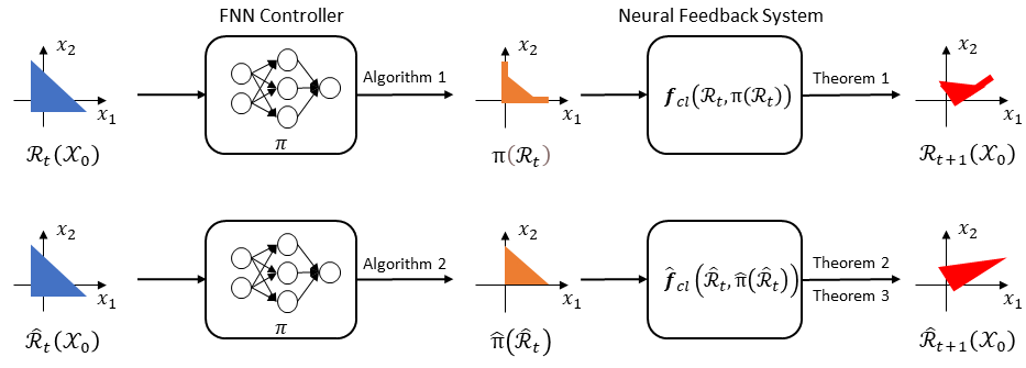
In this work, we leverage the properties of constrained zonotopes and deploy set-based analysis techniques to verify the safety of neural feedback systems, which are dynamical systems with a given ReLU-activated feedforward neural network (FNN) as the feedback controller. The contributions of this work are at least threefold: (i) Based on the output reachability analysis of FNNs, two novel methods are proposed to compute the exact and over-approximated reachable sets of neural feedback systems; (ii) LP-based sufficient conditions are proposed to verify the avoidance of unsafe sets for neural feedback systems; (iii) The proposed reachability analysis and safety verification methods are extended to neural feedback systems with nonlinear models. An overview of the proposed framework is illustrated in Figure 1.

The remainder of the paper is laid out as follows: Section II introduces preliminaries on constrained zonotopes and interval arithmetics and presents the problem statement. Section III introduces the constrained zonotope-based output analysis of FNNs in isolation. Section IV presents two reachable set computation methods for linear discrete-time systems with FNN controllers as well as two corresponding sufficient conditions to certify the safety of the neural feedback systems. Section V extends the reachability analysis and safety verification to systems with nonlinear models. Two numerical examples are shown in Section VI before the paper is concluded in Section VII.

Refer to caption — Fig. 1: The top (resp. bottom) flowchart illustrates the exact (resp. over-approximated) constrained zonotope-based reachability analysis, where $\mathcal{R}_{t}(\mathcal{X}_{0})$ (resp. $\hat{\mathcal{R}}_{t}(\mathcal{X}_{0})$ ) denotes the exact (resp. over-approximated) reachable set at time $t$ from initial set $\mathcal{X}_{0}$ , $\pi(\mathcal{R}_{t})$ (resp. $\hat{\pi}(\hat{\mathcal{R}}_{t})$ ) denotes the exact (resp. over-approximated) output set of the FNN controller, and $\bm{f}_{cl}$ (resp. $\hat{\bm{f}}_{cl}$ ) is the exact (resp. over-approximated) reachability mapping for the closed-loop neural feedback system.

II Preliminaries & Problem Statement

II-A Constrained Zonotope

Definition 1

[21] A set $\mathcal{Z}\subset\mathbb{R}^{n}$ is a constrained zonotope if there exists $(\mathbf{c},\mathbf{G},\mathbf{A},\mathbf{b})\in\mathbb{R}^{n}\times\mathbb{R}^{n\times n_{G}}\times\mathbb{R}^{n_{A}\times n_{G}}\times\mathbb{R}^{n_{A}}$ such that $\mathcal{Z}=\left\{\mathbf{G}\bm{\xi}+\mathbf{c}\;|\;\|\bm{\xi}\|_{\infty}\leq 1,\mathbf{A}\bm{\xi}=\mathbf{b}\right\}.$

Denote the constrained zonotope defined by $(\mathbf{c},\mathbf{G},\mathbf{A},\mathbf{b})$ as $CZ\{\mathbf{c},\mathbf{G},\mathbf{A},\mathbf{b}\}$ . Denote the unit hypercube by $B_{\infty}$ and define $B_{\infty}(\mathbf{A},\mathbf{b})=\{\bm{\xi}\in B_{\infty}\;|\;\mathbf{A}\bm{\xi}=\mathbf{b}\}$ . It’s proven that a constrained zonotope is equivalent to a convex polytope [21, Theorem 1]. Constrained zonotopes are closed under linear map, Minkowski sum and intersection as shown in the following result.

Lemma 1

[21, Proposition 1] For every $\mathbf{R}\in\mathbb{R}^{k\times n}$ , $\mathcal{Z}=CZ\left\{\mathbf{c}_{z},\mathbf{G}_{z},\mathbf{A}_{z},\mathbf{b}_{z}\right\}\subset\mathbb{R}^{n}$ , and $\mathcal{W}=CZ\{\mathbf{c}_{w},\mathbf{G}_{w},\mathbf{A}_{w},$ $\mathbf{b}_{w}\}\subset\mathbb{R}^{n}$ , the following three identities hold:

	$\displaystyle\mathbf{R}\mathcal{Z}$	$\displaystyle=CZ\left\{\mathbf{R}\mathbf{c}_{z},\mathbf{RG}_{z},\mathbf{A}_{z},\mathbf{b}_{z}\right\},$
	$\displaystyle\mathcal{Z}\oplus\mathcal{W}$	$\displaystyle=CZ\left\{\mathbf{c}_{z}+\mathbf{c}_{w},[\mathbf{G}_{z}\;\mathbf{G}_{w}],\begin{bmatrix}\mathbf{A}_{z}&\mathbf{0}\\ \mathbf{0}&\mathbf{A}_{w}\end{bmatrix},\begin{bmatrix}\mathbf{b}_{z}\\ \mathbf{b}_{w}\end{bmatrix}\right\},$
	$\displaystyle\mathcal{Z}\cap\mathcal{W}$	$\displaystyle=CZ\left\{\mathbf{c}_{z},[\mathbf{G}_{z}\;\mathbf{0}],\begin{bmatrix}\mathbf{A}_{z}&\mathbf{0}\\ \mathbf{0}&\mathbf{A}_{w}\\ \mathbf{G}_{z}&-\mathbf{G}_{w}\end{bmatrix},\begin{bmatrix}\mathbf{b}_{z}\\ \mathbf{b}_{w}\\ \mathbf{c}_{w}-\mathbf{c}_{z}\end{bmatrix}\right\},$

where $\oplus$ denotes the Minkowski sum.

Checking the emptiness of a constrained zonotope requires the solution of a LP.

Lemma 2

[21, Proposition 2] For every $\mathcal{Z}=CZ\{\mathbf{c},\mathbf{G},$ $\mathbf{A},\mathbf{b}\}\subset\mathbb{R}^{n}$ , $\mathcal{Z}\not=\emptyset$ iff $\min\{||\bm{\xi}||_{\infty}\;|\;\mathbf{A}\bm{\xi}=\mathbf{b}\}\leq 1.$

The intersection of a constrained zonotope and a halfspace is still a constrained zonotope as shown in the following result.

Lemma 3

[22, Theorem 1] If the constrained zonotope $\mathcal{Z}=CZ\{\mathbf{c},\mathbf{G},\mathbf{A},\mathbf{b}\}\subset\mathbb{R}^{n}$ intersects the hyperplane $\mathcal{H}=\left\{\bm{x}\in\mathbb{R}^{n}\mid\mathbf{h}^{T}\bm{x}=f\right\}$ corresponding to the halfspace $\mathcal{H}_{-}=\left\{\bm{x}\in\mathbb{R}^{n}\mid\mathbf{h}^{T}\bm{x}\leq f\right\}$ , then the intersection $\mathcal{Z}_{h}=\mathcal{Z}\cap\mathcal{H}_{-}$ is a constrained zonotope

\displaystyle\mathcal{Z}_{h}=\left\{\mathbf{c},\begin{bmatrix}\mathbf{G}&\mathbf{0}\end{bmatrix},\begin{bmatrix}\mathbf{A}&\mathbf{0}\\ \mathbf{h}^{T}\mathbf{G}&\frac{d_{m}}{2}\end{bmatrix},\begin{bmatrix}\mathbf{b}\\ f-\mathbf{h}^{T}\mathbf{c}-\frac{d_{m}}{2}\end{bmatrix}\right\}

where $d_{m}=f-\mathbf{h}^{T}\mathbf{c}+\sum_{i=1}^{n_{G}}\left|\mathbf{h}^{T}\mathbf{G}[:,i]\right|$ and $\mathbf{G}[:,i]$ is the $i$ -th column of matrix $\mathbf{G}$ .

In the following, we denote $\mathbf{e}_{i}$ as the $i$ -th canonical vector, $\mathcal{H}^{i}=\{\bm{x}\in\mathbb{R}^{n}\mid\mathbf{e}_{i}^{T}\bm{x}=0\}$ , $\mathcal{H}^{i}_{-}=\{\bm{x}\in\mathbb{R}^{n}\mid\mathbf{e}_{i}^{T}\bm{x}\leq 0\}$ , and $\mathcal{H}^{i}_{+}=\{\bm{x}\in\mathbb{R}^{n}\mid\mathbf{e}_{i}^{T}\bm{x}\geq 0\}$ for $i=1,\dots,n$ .

II-B Interval Arithmetic

A real interval $[a]=[\underline{a},\bar{a}]$ is a subset of $\mathbb{R}$ . Denote $\mathbb{IR}$ , $\mathbb{IR}^{n}$ and $\mathbb{IR}^{n\times m}$ as the set of all real intervals of $\mathbb{R}$ , all $n$ -dimensional real interval vectors and all $n\times m$ real interval matrices, respectively. Real arithmetic operations on $\mathbb{R}$ can be extended to $\mathbb{IR}$ as follows: for $\circ\in\{+,-,*,\div\}$ , $[a]\circ[b]=\{\inf_{x\in[a],y\in[b]}x\circ y,\sup_{x\in[a],y\in[b]}x\circ y\}$ . The classical operations for real vectors and real matrices can be directly extended to interval vectors and interval matrices [23, 24].

For a bounded set $\mathcal{X}\subset\mathbb{R}^{n}$ , denote $\Box\mathcal{X}$ as the interval hull of $\mathcal{X}$ . The interval hull $\Box\mathcal{Z}$ of a constrained zonotope $\mathcal{Z}$ can be computed using the LP proposed in [21, 25]. Denote $\lhd([\mathbf{J}],\mathcal{Z})$ as the operation of computing a constrained zonotopic enclosure of the product of an interval matrix $[\mathbf{J}]$ and a constrained zonotope $\mathcal{Z}$ using [25, Theorem 1].

II-C Problem Statement

We consider the following discrete-time control system:

\bm{x}{(t+1)}=\bm{f}(\bm{x}(t))+B_{d}\bm{u}(t)

(1)

where $\bm{x}(t)\in\mathcal{X}\subseteq\mathbb{R}^{n}$ is the state, $\bm{u}(t)\in\mathbb{R}^{m}$ is the control input, $\bm{f}:\mathcal{X}\rightarrow\mathbb{R}^{n}$ is a twice continuously differentiable vector-valued function (i.e., $\bm{f}$ is of class $\mathcal{C}^{2}$ ), and $B_{d}\in\mathbb{R}^{n\times m}$ is a given input matrix. Given an initial state $\bm{x}(0)$ and a control sequence $\bm{u}=\bm{u}(0),\bm{u}(1),\dots$ , the state trajectory of system (1) is denoted as $\bm{x}=\bm{x}(0),\bm{x}(1),\dots$ .

Assume that the controller in (1) is a state-feedback controller $\bm{u}(t)=\pi(\bm{x}(t))$ that is parameterized by an $\ell$ -layer FNN with the Rectified Linear Unit (ReLU) activation function. Letting $\bm{x}^{(0)}=\bm{x}(t)$ and using the notation from [11], for each layer $k=1,\dots,\ell-1$ , the neuron of the FNN is given by

\bm{x}^{(k)}=ReLU\left(\mathcal{L}\left(\bm{x}^{(k-1)},\mathbf{W}^{(k-1)},\mathbf{v}^{(k-1)}\right)\right)

(2)

where $\mathbf{W}^{(k-1)}$ is the $k$ -th layer weight matrix, $\mathbf{v}^{(k-1)}$ is the $k$ -th layer bias vector, $\mathcal{L}(\bm{x},\mathbf{W},\mathbf{v})=\mathbf{W}\bm{x}+\mathbf{v}$ , and $ReLU(\bm{x})=\max\{0,\bm{x}\}$ . In the last layer, only the linear operation is applied, i.e., $\pi(\bm{x}(t))=\bm{x}^{(\ell)}=\mathcal{L}(\bm{x}^{(\ell-1)},\mathbf{W}^{(\ell-1)},\mathbf{v}^{(\ell-1)})$ .

The closed-loop system with dynamics (1) and the controller $\bm{u}(t)=\pi(\bm{x}(t))$ becomes:

\bm{x}{(t+1)}=\bm{f}(\bm{x}(t))+B_{d}\pi(\bm{x}(t)).

(3)

Given a set of initial states $\mathcal{X}_{0}\subseteq\mathbb{R}^{n}$ , the (forward) reachable set of closed-loop system (3) at time $t$ from the set $\mathcal{X}_{0}$ is denoted as $\mathcal{R}_{t}(\mathcal{X}_{0})\triangleq\{\bm{x}(t)\in\mathbb{R}^{n}|\bm{x}(0)\in\mathcal{X}_{0},\bm{x}{(k+1)}=\bm{f}(\bm{x}(k))+B_{d}\pi(\bm{x}(k)),k=0,1,\dots,t-1\}$ , or simply $\mathcal{R}_{t}$ when $\mathcal{X}_{0}$ is clear from context. Denote an over-approximation of the set $\mathcal{R}_{t}(\mathcal{X}_{0})$ as $\hat{\mathcal{R}}_{t}(\mathcal{X}_{0})$ .

In this paper, we investigate the following problems in which the initial set and the unsafe sets are all assumed to be in the form of constrained zonotopes.

Problem 1

Given an initial set $\mathcal{X}_{0}$ that is represented as a constrained zonotope, the parameters for the FNN controller $\pi$ and a time horizon $T\in\mathbb{Z}_{>0}$ , compute the exact reachable set $\mathcal{R}_{t}(\mathcal{X}_{0})$ or an over-approximated reachable set $\hat{\mathcal{R}}_{t}(\mathcal{X}_{0})$ for the closed-loop system (3) where $t=1,2,\dots,T$ .

Problem 2

Given unsafe sets $\{\mathcal{O}_{1},\mathcal{O}_{2},\dots,\mathcal{O}_{N}\}$ where $\mathcal{O}_{i}(1\leq i\leq N)$ is represented as a constrained zonotope, verify whether the state trajectory of the closed-loop system (3) can avoid the unsafe regions for $t=1,2,\dots,T$ .

III Output Analysis of FNNs Based On Constrained Zonotopes

III-A Exact Output Analysis

In this subsection, we will compute the exact output set for a given FNN shown in (2) with an input set represented as a constrained zonotope.

From the definition of the FNN in (2), one can see that the output set of an FNN can be derived layer by layer as the output of layer $k$ is the input of layer $k+1$ , for $k=1,\dots,\ell-1$ . Therefore, we will focus on finding the input-output relationship for one layer. From Lemma 1, if we pass an input represented as a constrained zonotope $\mathcal{Z}=CZ\{\mathbf{c},\mathbf{G},\mathbf{A},\mathbf{b}\}$ through a linear layer, then we will obtain the output as $\mathcal{L}(\mathcal{Z},\mathbf{W},\mathbf{v})=CZ\{\mathbf{W}\mathbf{c}+\mathbf{v},\mathbf{W}\mathbf{G},\mathbf{A},\mathbf{b}\}$ . Thus, the only difficulty remaining is to find the output when passing through the ReLU activation function. In [12], an algorithm is proposed to compute the exact output set for a single neural network layer using the star sets representation. It can be shown that constrained zonotope is a special case of star sets [26]. Therefore, we can apply the algorithm in [12] to compute the exact output set using constrained zonotopes. The details are summarized in Algorithm 1 for which both the input set and the output set are in the form of constrained zonotopes.

Algorithm 1 reveals that given a constrained zonotope as the input set $\mathcal{Z}$ to the FNN $\pi$ , the exact output of the FNN can be represented as a union of constrained zonotopes: $\pi(\mathcal{Z})=\bigcup_{i=1}^{n_{\pi}}CZ\{\mathbf{c}_{i},\mathbf{G}_{i},\mathbf{A}_{i},\mathbf{b}_{i}\},$ where $n_{\pi}$ depends on the depth of the FNN $\pi$ , the number of neurons and the output intersections with halfspaces.

Input: weight matrix

\mathbf{W}

, bias vector

\mathbf{v}

, constrained zonotope input sets

\mathcal{Z}=\mathcal{Z}_{1}\cup\mathcal{Z}_{2}\cup\dots\cup\mathcal{Z}_{N_{z}}

Output: exact output set

\mathcal{R}

Function $\mathcal{R}$ = ReachNN( $\mathcal{Z}$ , $\mathbf{W}$ , $\mathbf{v}$ ): 3

\mathcal{R}=\emptyset

for $h=1:N_{z}$ do 4

\mathcal{I}=\mathbf{W}\mathcal{Z}_{h}+\mathbf{v}

[lb\quad up]\leftarrow

range of

\bm{x}

\mathcal{I}

map=find(lb<0)

for $i$ in $map$ do 5

\mathcal{I}=\textnormal{{StepReLU}}(\mathcal{I},i,lb[i],up[i])

\mathcal{R}=\mathcal{R}\cup\mathcal{I}

return

\mathcal{R}

Function $\tilde{\mathcal{I}}$ = StepReLU( ${\mathcal{I}}$ , $i$ , $lb_{i}$ , $up_{i}$ ): 7

{\mathcal{I}}=\mathcal{I}_{1}\cup\mathcal{I}_{2}\cup\cdots\cup\mathcal{I}_{N_{I}}\subset\mathbb{R}^{n_{I}}

\tilde{\mathcal{I}}=\emptyset

\mathbf{E}_{i}=[\mathbf{e}_{1}\;\cdots\;\mathbf{e}_{i-1}\;\mathbf{0}\;\mathbf{e}_{i+1}\;\cdots\;\mathbf{e}_{n_{I}}]

for $j=1:N_{I}$ do 8

if $up_{i}\leq 0$ then 9

\hat{\mathcal{I}}=\mathbf{E}_{i}{\mathcal{I}}_{j}

if $lb_{i}<0\;\&\;up_{i}>0$ then 10

\mathcal{I}_{+}={\mathcal{I}}_{j}\cap\mathcal{H}^{i}_{+}

\mathcal{I}_{-}={\mathcal{I}}_{j}\cap\mathcal{H}^{i}_{-}

\hat{\mathcal{I}}=\mathcal{I}_{+}\cup\mathbf{E}_{i}\mathcal{I}_{-}

\tilde{\mathcal{I}}=\tilde{\mathcal{I}}\cup\hat{\mathcal{I}}

return

\tilde{\mathcal{I}}

Algorithm 1 (Adapted from Algorithm 3.1 in [12]) Exact output analysis for one layer of FNN

III-B Over-approximation Output Analysis

One major drawback of Algorithm 1 is that in the worst scenario, the number of constrained zonotopes in the output set will grow exponentially with the number of layers and the number of neurons. Thus, it will dramatically increase the computation burden of output analysis for deep neural networks. In this subsection, we will introduce an algorithm that can over-approximate the output set of an FNN with one constrained zonotope. Similar to the over-approximation methods developed for star sets in [12], we construct the output set of each layer of the FNN as a constrained zonotope using a triangle over-approximation of the ReLU activation function for each neuron. As noted in [12], the star-based over-approximation algorithm is much less conservative than the zonotope-based [10] and abstract domain [27] based approaches in approximating the ReLU function.

Figure 2 shows the main idea of ReLU function over-approximation. Given a range of the $i$ -th neuron $\bm{x}[i]$ as $[lb_{i},up_{i}]$ , the output of the ReLU activation function can be divided into two parts (i.e., $I_{1}$ and $I_{2}$ ) that can be covered by the gray triangle area $\hat{I}$ (including the boundaries) which is the intersection of three halfspaces: $\bm{y}[i]-\bm{x}[i]\geq 0$ , $\bm{x}[i]\geq 0$ and $(up_{i}-lb_{i})\bm{y}[i]-up_{i}(\bm{x}[i]-lb_{i})\leq 0$ . Using this convex relaxation, we modify Algorithm 1 and design Algorithm 2 to compute the over-approximated output set as a single constrained zonotope at each time step.

Remark 1

From Line 14 to Line 19 in Algorithm 2, we know that if the lower bound of the neuron is negative and the upper bound of the neuron is positive, then the algorithm will introduce four new variables and three new equality constraints. In the worst case, if we have totally $M$ number of neurons in the FNN, the number of new variables in the over-approximated output set will be $4M$ and the number of new constraints will be $3M$ . This could cause a computational burden issue for a deep FNN. However, it’s possible to utilize the order reduction methods proposed in [21, 22] to reduce the complexity of the approximated constrained zonotopes.

Input: weight matrix

\mathbf{W}

, bias vector

\mathbf{v}

, constrained zonotope input set

\mathcal{Z}

Output: over-approximated output set

\hat{\mathcal{R}}

Function $\hat{\mathcal{R}}$ = OverReachNN( $\mathcal{Z}$ , $\mathbf{W}$ , $\mathbf{v}$ ): 3

\mathcal{I}=\mathbf{W}\mathcal{Z}+\mathbf{v}

[lb\quad up]\leftarrow

range of

\bm{x}

\mathcal{I}

map=find(lb<0)

for $i$ in $map$ do 4

\mathcal{I}=\textnormal{{OverStepReLU}}(\mathcal{I},i,lb[i],up[i])

return

\hat{\mathcal{R}}=\mathcal{I}

Function $\hat{\mathcal{I}}$ = OverStepReLU( ${\mathcal{I}}$ , $i$ , $l_{i}$ , $u_{i}$ ): 6

\mathcal{I}=CZ\{\mathbf{c},\mathbf{G},\mathbf{A},\mathbf{b}\}\subset\mathbb{R}^{n_{I}}

\mathbf{E}_{i}=[\mathbf{e}_{1}\;\cdots\;\mathbf{e}_{i-1}\;\mathbf{0}\;\mathbf{e}_{i+1}\;\cdots\;\mathbf{e}_{n_{I}}]

if $u_{i}\leq 0$ then 7

\hat{\mathcal{I}}=\mathbf{E}_{i}{\mathcal{I}}

if $l_{i}<0\;\&\;u_{i}>0$ then 8

\hat{\mathbf{c}}=\mathbf{E}_{i}\mathbf{c}

\hat{\mathbf{G}}=\begin{bmatrix}\mathbf{E}_{i}\mathbf{G}&u_{i}\mathbf{e}_{i}&\mathbf{0}_{n_{I}\times 1}&\mathbf{0}_{n_{I}\times 1}&\mathbf{0}_{n_{I}\times 1}\end{bmatrix}

\hat{\mathbf{A}}=\begin{bmatrix}\mathbf{A}&\mathbf{0}_{n_{A}\times 1}&\mathbf{0}_{n_{A}\times 1}&\mathbf{0}_{n_{A}\times 1}&\mathbf{0}_{n_{A}\times 1}\\ \mathbf{0}_{1\times n_{G}}&1&1&0&0\\ -\mathbf{G}[i,:]&u_{i}&0&u_{i}-l_{i}&0\\ -\mathbf{G}[i,:]&u_{i}-l_{i}&0&0&u_{i}-l_{i}\end{bmatrix}

\hat{\mathbf{b}}=\begin{bmatrix}\mathbf{b}&1&\mathbf{c}[i]+u_{i}-l_{i}&\mathbf{c}[i]-u_{i}\end{bmatrix}^{T}

\hat{\mathcal{I}}=CZ\{\hat{\mathbf{c}},\hat{\mathbf{G}},\hat{\mathbf{A}},\hat{\mathbf{b}}\}

return

\hat{\mathcal{I}}

Algorithm 2 Over-approximated output analysis for one layer of FNN

IV Reachability analysis and Safety Verification for Neural Feedback System with Linear Model

In this section, we consider a neural feedback system with a linear model and an FNN controller expressed as follows:

\bm{x}{(t+1)}=A_{d}\bm{x}(t)+B_{d}\pi(\bm{x}(t))

(4)

where $A_{d}\in\mathbb{R}^{n\times n}$ is a given state matrix and other terms are the same as defined in (1).

IV-A Reachability Analysis

IV-A1 Exact Reachability Analysis

Given an initial set $\mathcal{X}_{0}$ as a constrained zonotope, Algorithm 1 and 2 can be used to compute the exact and over-approximated output set of FNN $\pi(\mathcal{X}_{0})$ respectively. Now we consider the problem of computing the reachable sets $\mathcal{R}_{t}(\mathcal{X}_{0}),\;t=1,2,\dots,T,$ for the closed-loop system (4). Let $\mathcal{R}_{0}(\mathcal{X}_{0})=\mathcal{X}_{0}$ and $\bm{f}_{cl}(\bm{x})=A_{d}\bm{x}+B_{d}\pi(\bm{x})$ . A trivial idea is to compute separately the two terms on the right hand side of (4) by using Lemma 1 and then take their Minkowski sum; however, the resulting set will be a conservative over-approximation of the true reachable set.

In the following theorem, we present the exact form of $\bm{f}_{cl}(\mathcal{Z})$ for a given constrained zonotope $\mathcal{Z}$ .

Theorem 1

\bm{f}_{cl}(\mathcal{Z})=\cup_{i=1}^{n_{\pi}}CZ\{\mathbf{c}_{i}^{cl},\mathbf{G}_{i}^{cl},\mathbf{A}_{i}^{cl},\mathbf{b}_{i}^{cl}\}

(5)

where

	$\displaystyle\mathbf{G}_{i}^{cl}$	$\displaystyle=A_{d}\begin{bmatrix}\mathbf{G}&\mathbf{0}_{n\times(n_{G_{i}}-n_{G})}\end{bmatrix}+B_{d}\mathbf{G}_{i},$
	$\displaystyle\mathbf{c}_{i}^{cl}$	$\displaystyle=A_{d}\mathbf{c}+B_{d}\mathbf{c}_{i},\;\mathbf{A}_{i}^{cl}=\mathbf{A}_{i},\;\mathbf{b}_{i}^{cl}=\mathbf{b}_{i}.$

Proof:

Denote the right hand side of (5) as ${\mathcal{Z}}_{R}$ . Firstly we prove $\bm{f}_{cl}(\mathcal{Z})\subseteq{\mathcal{Z}}_{R}$ . Let $\bm{x}$ be any element of set $\mathcal{Z}$ , i.e., $\bm{x}\in\mathcal{Z}$ . We know there exists $\bm{\xi}_{1}$ such that $\bm{x}=\mathbf{c}+\mathbf{G}\bm{\xi}_{1}$ , $||\bm{\xi}_{1}||_{\infty}\leq 1$ and $\mathbf{A}\bm{\xi}_{1}=\mathbf{b}$ . From the procedures in Algorithm 1 and Lemma 3, it’s easy to check that $n_{G_{i}}\geq n_{G}$ and the $(n_{G}+1)$ -th to the $n_{G_{i}}$ -th columns of $G_{i}$ are all zeros. Also, the first $n_{A}$ rows of $\mathbf{A}_{i}$ are $\begin{bmatrix}\mathbf{A}&\mathbf{0}_{(n_{G_{i}}-n_{G})\times n_{A}}\end{bmatrix}$ and the first $n_{A}$ rows of $\mathbf{b}_{i}$ are $\mathbf{b}$ .

Since $\pi(\bm{x})\in\pi(\mathcal{Z})$ , there must exist $i\in\{1,2,\dots,n_{\pi}\}$ such that $\pi(\bm{x})\in CZ\{\mathbf{c}_{i},\mathbf{G}_{i},\mathbf{A}_{i},\mathbf{b}_{i}\}$ . Thus, we know there exists $\bm{\xi}=\begin{bmatrix}\bm{\xi}_{1}^{T}&\bm{\xi}_{2}^{T}\end{bmatrix}^{T}$ such that $\bm{\xi}\in B_{\infty}(\mathbf{A}_{i},\mathbf{b}_{i})$ and $\pi(\bm{x})=\mathbf{c}_{i}+\mathbf{G}_{i}\bm{\xi}$ . Therefore, $\bm{f}_{cl}(\bm{x})=A_{d}\bm{x}+B_{d}\pi(\bm{x})=A_{d}(\mathbf{c}+\mathbf{G}\bm{\xi}_{1})+B_{d}(\mathbf{c}_{i}+\mathbf{G}_{i}\begin{bmatrix}\bm{\xi}_{1}^{T}&\bm{\xi}_{2}^{T}\end{bmatrix}^{T})=(A_{d}\mathbf{c}+B_{d}\mathbf{c}_{i})+(A_{d}\begin{bmatrix}\mathbf{G}&\mathbf{0}_{n\times(n_{G_{i}}-n_{G})}\end{bmatrix}+B_{d}\mathbf{G}_{i})\bm{\xi}=\mathbf{c}_{i}^{cl}+\mathbf{G}_{i}^{cl}\bm{\xi}$ , where $\bm{\xi}\in B_{\infty}(\mathbf{A}_{i},\mathbf{b}_{i})=B_{\infty}(\mathbf{A}_{i}^{cl},\mathbf{b}_{i}^{cl})$ . Then, we have $\bm{f}_{cl}(\bm{x})\in CZ\{\mathbf{c}_{i}^{cl},\mathbf{G}_{i}^{cl},\mathbf{A}_{i}^{cl},\mathbf{b}_{i}^{cl}\}\subseteq{\mathcal{Z}}_{R}$ . Since $\bm{x}$ is arbitrary, we know that $\bm{f}_{cl}(\mathcal{Z})\subseteq{\mathcal{Z}}_{R}$ .

Next, we show that ${\mathcal{Z}}_{R}\subseteq\bm{f}_{cl}(\mathcal{Z})$ . Let $\bm{z}\in{\mathcal{Z}}_{R}$ . Then, $\exists i\in\{1,2,\dots,n_{\pi}\}$ such that $\bm{z}\in CZ\{\mathbf{c}_{i}^{cl},\mathbf{G}_{i}^{cl},\mathbf{A}_{i}^{cl},\mathbf{b}_{i}^{cl}\}$ . Therefore, $\exists\bm{\xi}\in B_{\infty}(\mathbf{A}_{i}^{cl},\mathbf{b}_{i}^{cl})$ such that $\bm{z}=\mathbf{c}_{i}^{cl}+\mathbf{G}_{i}^{cl}\bm{\xi}=A_{d}\mathbf{c}+B_{d}\mathbf{c}_{i}+(A_{d}\begin{bmatrix}\mathbf{G}&\mathbf{0}_{n\times(n_{G_{i}}-n_{G})}\end{bmatrix}+B_{d}\mathbf{G}_{i})\bm{\xi}$ . Partitioning $\bm{\xi}$ as $\bm{\xi}=\begin{bmatrix}\bm{\xi}_{1}^{T}&\bm{\xi}_{2}^{T}\end{bmatrix}^{T}$ , it follows that $\bm{\xi}_{1}\in B_{\infty}(\mathbf{A},\mathbf{b})$ , $\bm{z}=A_{d}\mathbf{c}+(A_{d}\begin{bmatrix}\mathbf{G}&\mathbf{0}_{n\times(n_{G_{i}}-n_{G})}\end{bmatrix}\begin{bmatrix}\bm{\xi}_{1}^{T}&\bm{\xi}_{2}^{T}\end{bmatrix}^{T}+B_{d}\mathbf{c}_{i}+B_{d}\mathbf{G}_{i}\bm{\xi}=A_{d}\mathbf{c}+A_{d}\mathbf{G}\bm{\xi}_{1}+B_{d}\mathbf{c}_{i}+B_{d}\mathbf{G}_{i}\bm{\xi}$ . Let $\bm{x}=\mathbf{c}+\mathbf{G}\bm{\xi}_{1}$ , then $\pi(\bm{x})=\mathbf{c}_{i}+\mathbf{G}_{i}\bm{\xi}$ , which implies $\bm{x}\in\mathcal{Z}$ . Thus, $\bm{z}=A_{d}\bm{x}+B_{d}\pi(\bm{x})=\bm{f}_{cl}(\bm{x})\in\bm{f}_{cl}(\mathcal{Z})$ . Since $\bm{z}$ is arbitrary, ${\mathcal{Z}}_{R}\subseteq\bm{f}_{cl}(\mathcal{Z})$ . Thus, we conclude that $\bm{f}_{cl}(\mathcal{Z})={\mathcal{Z}}_{R}$ . ∎

Theorem 1 can be extended to the case where the input set is a union of constrained zonotopes as shown below.

Corollary 1

Given a union of $M$ constrained zonotopes $\mathcal{Z}=\cup_{j=1}^{M}\mathcal{Z}_{j}\subset\mathbb{R}^{n}$ , where $\mathcal{Z}_{j}=CZ\{\mathbf{c}_{j},\mathbf{G}_{j},\mathbf{A}_{j},\mathbf{b}_{j}\}$ . Let $\pi(\mathcal{Z}_{j})=\cup_{i=1}^{n_{\pi,j}}CZ\{\mathbf{c}_{i,j},\mathbf{G}_{i,j},\mathbf{A}_{i,j},\mathbf{b}_{i,j}\}$ be the computed output set using Algorithm 1 and set $\mathcal{Z}_{j}$ for $j=1,2,\dots,M$ . Then,

	$\displaystyle\bm{f}_{cl}(\mathcal{Z})=$	$\displaystyle\cup_{j=1}^{M}\bm{f}_{cl}(\mathcal{Z}_{j})$		(6)
	$\displaystyle=$	$\displaystyle\cup_{j=1}^{M}\cup_{i=1}^{n_{\pi,j}}CZ\{\mathbf{c}_{i,j}^{cl},\mathbf{G}_{i,j}^{cl},\mathbf{A}_{i,j}^{cl},\mathbf{b}_{i,j}^{cl}\},$		(6)

where $\mathbf{A}_{i,j}^{cl}=\mathbf{A}_{i,j}$ , $\mathbf{b}_{i,j}^{cl}=\mathbf{b}_{i,j}$ , $\mathbf{c}_{i,j}^{cl}=A_{d}\mathbf{c}_{j}+B_{d}\mathbf{c}_{i,j}$ , and $\mathbf{G}_{i,j}^{cl}=A_{d}[\mathbf{G}_{j}\;\mathbf{0}_{n\times(n_{G_{i,j}}-n_{G_{j}})}]+B_{d}\mathbf{G}_{i,j}$ , with $n_{G_{j}}$ the number of columns of $\mathbf{G}_{j}$ and $n_{G_{i,j}}$ the number of columns of $\mathbf{G}_{i,j}$ .

Using Theorem 1 and Corollary 1, we can compute the exact reachable sets of closed-loop system (4) as follows:

	$\displaystyle\mathcal{R}_{0}$	$\displaystyle=\mathcal{X}_{0},$		(7)
	$\displaystyle\mathcal{R}_{t}$	$\displaystyle=\bm{f}_{cl}(\mathcal{R}_{t-1}),\;t=1,\dots,T.$		(7)

Remark 2

In [17, 18], over-approximation reachability computation algorithms are proposed for discrete-time systems with FNN controllers. The main idea there is to bound the nonlinearities of FNNs with quadratic or linear constraints. In contrast, the method proposed in this work includes the FNN nonlinearities in the set-based operations, and therefore, provides a different way for handling reachability analysis of neural feedback systems without bounding or relaxing the FNN nonlinearities.

The price of accuracy, however, is that the number of constrained zonotopes and the order of constrained zonotopes will grow exponentially. Thus, order reduction techniques as proposed in [21, 22] are needed for analyzing deep neural networks. Nevertheless, as shown in Section VI, the computation time of our exact analysis algorithm is comparable with other state-of-the-art algorithms.

IV-A2 Over-approximation Reachability Analysis

It is computationally demanding to carry out the exact reachability analysis based on (7) when $n_{\pi}$ , which depends on the depth and width of the FNN, is large. The following theorem shows that an over-approximated reachable set can be computed by using Algorithm 2, to achieve a trade-off between accuracy and efficiency for the reachability analysis.

Theorem 2

Given any constrained zonotope $\mathcal{Z}=CZ\{\mathbf{c},\mathbf{G},\mathbf{A},\mathbf{b}\}\subset\mathbb{R}^{n}$ , $\mathbf{G}\in\mathbb{R}^{n\times n_{G}}$ , $\mathbf{A}\in\mathbb{R}^{n_{A}\times n_{G}}$ , let $\hat{\pi}(\mathcal{Z})$ be the computed output set using Algorithm 2, i.e., $\hat{\pi}(\mathcal{Z})=CZ\{\hat{\mathbf{c}},\hat{\mathbf{G}},\hat{\mathbf{A}},\hat{\mathbf{b}}\}\supseteq\pi(\mathcal{Z})$ . Let $n_{\hat{G}}$ be the number of columns of $\hat{\mathbf{G}}$ . Then, an over-approximated range of $\bm{f}_{cl}(\mathcal{Z})$ can be computed as:

\hat{\bm{f}}_{cl}(\mathcal{Z})=CZ\{\hat{\mathbf{c}}_{cl},\hat{\mathbf{G}}_{cl},\hat{\mathbf{A}}_{cl},\hat{\mathbf{b}}_{cl}\}\supseteq\bm{f}_{cl}(\mathcal{Z})

(8)

where

	$\displaystyle\hat{\mathbf{G}}_{cl}$	$\displaystyle=A_{d}\begin{bmatrix}\mathbf{G}&\mathbf{0}_{n\times(n_{\hat{G}}-n_{G})}\end{bmatrix}+B_{d}\hat{\mathbf{G}},$
	$\displaystyle\hat{\mathbf{c}}_{cl}$	$\displaystyle=A_{d}\mathbf{c}+B_{d}\hat{\mathbf{c}},\;\hat{\mathbf{A}}_{cl}=\hat{\mathbf{A}},\;\hat{\mathbf{b}}_{cl}=\hat{\mathbf{b}}.$

Proof:

From the construction of $\hat{\mathbf{G}}$ in Algorithm 2 Line 17, we have that $n_{\hat{G}}\geq n_{G}$ . For any $\bm{x}\in\mathcal{Z}$ , $\exists\bm{\xi}_{1}$ such that $\bm{x}=\mathbf{c}+\mathbf{G}\bm{\xi}_{1}$ and $\bm{\xi}_{1}\in B_{\infty}(\mathbf{A},\mathbf{b})$ . Since $\pi(\bm{x})\in\pi(\mathcal{Z})\subseteq\hat{\pi}(\mathcal{Z})$ , there exists $\bm{\xi}=\begin{bmatrix}\bm{\xi}_{1}^{T}&\bm{\xi}_{2}^{T}\end{bmatrix}^{T}$ such that $\pi(\bm{x})=\hat{\mathbf{c}}+\hat{\mathbf{G}}\bm{\xi}$ and $\bm{\xi}\in B_{\infty}(\hat{\mathbf{A}},\hat{\mathbf{b}})$ . Thus, similar to the proof of Theorem 1, we have $\bm{f}_{cl}(\bm{x})=\hat{\mathbf{c}}_{cl}+\hat{\mathbf{G}}_{cl}\bm{\xi}$ where $\bm{\xi}\in B_{\infty}(\hat{\mathbf{A}},\hat{\mathbf{b}})$ . Therefore, $\bm{f}_{cl}(\bm{x})\in\hat{\bm{f}}_{cl}(\mathcal{Z})$ . Since $\bm{x}$ is arbitrary, we conclude that $\bm{f}_{cl}(\mathcal{Z})\subseteq\hat{\bm{f}}_{cl}(\mathcal{Z})$ . ∎

Using Theorem 2, we can compute the over-approximated reachable sets of closed-loop system (4) as follows:

	$\displaystyle\hat{\mathcal{R}}_{0}$	$\displaystyle=\mathcal{X}_{0}$		(9)
	$\displaystyle\hat{\mathcal{R}}_{t}$	$\displaystyle=\hat{\bm{f}}_{cl}(\hat{\mathcal{R}}_{t-1}),\;t=1,\dots,T.$		(9)

IV-B Safety Verification

Let the exact reachable set at time $t$ computed by (7) be $\mathcal{R}_{t}(\mathcal{X}_{0})=\cup^{n_{t}}_{i=1}\mathcal{R}_{t}^{i}(\mathcal{X}_{0})=\cup^{n_{t}}_{i=1}CZ\{\mathbf{c}_{i}^{t},\mathbf{G}_{i}^{t},\mathbf{A}_{i}^{t},\mathbf{b}_{i}^{t}\}$ for $t=1,2,\dots,T$ . Let the $N$ unsafe sets be $\mathcal{O}_{j}=CZ\{\mathbf{c}^{o}_{j},\mathbf{G}^{o}_{j},\mathbf{A}^{o}_{j},\mathbf{b}^{o}_{j}\}$ for $j=1,2,\dots,N$ . The following result provides a sufficient and necessary condition on the safety verification of the closed-loop system (4).

Proposition 1

Consider the reachable sets $\mathcal{R}_{1},\dots,\mathcal{R}_{T}$ and unsafe sets $\mathcal{O}_{1},\dots,\mathcal{O}_{N}$ defined above, the state trajectories of the closed-loop system (4) can avoid all the unsafe regions if and only if the following condition is satisfied:

		$\displaystyle\min\{\|\|\bm{\xi}\|\|_{\infty}\;\|\;\begin{bmatrix}\mathbf{A}_{i}^{t}&\mathbf{0}\\ \mathbf{0}&\mathbf{A}_{j}^{o}\\ \mathbf{G}_{i}^{t}&-\mathbf{G}_{j}^{o}\end{bmatrix}\bm{\xi}=\begin{bmatrix}\mathbf{b}_{i}^{t}\\ \mathbf{b}_{j}^{o}\\ \mathbf{c}_{j}^{o}-\mathbf{c}_{i}^{t}\end{bmatrix}\}>1,$		(10)
		$\displaystyle\forall t\in\{1,\dots,T\},\;\forall i\in\{1,\dots,n_{t}\},\;\forall j\in\{1,\dots,N\}.$

Proof:

Avoiding the unsafe regions can be equivalently expressed as none of the reachable sets intersect with any of the unsafe sets. According to Lemma 1, we know the intersection of the $i$ -th constrained zonotope from $\mathcal{R}_{t}$ and the $j$ -th unsafe set is also a constrained zonotope, i.e., R t i ∩O j = CZ{c i t , [ G i t 0 ] , [ A i t 0 0 A j o G i t -G j o ] , [ b i t b j o c j o - c i t ] }. Using Lemma 2, we have that $\mathcal{R}_{t}^{i}\cap\mathcal{O}_{j}$ is empty if and only if (10) is satisfied. Therefore, the avoidance of all unsafe regions can be certified if and only if (10) is satisfied for all $t\in\{1,\dots,T\}$ , $i\in\{1,\dots,n_{t}\}$ and $j\in\{1,\dots,N\}$ . ∎

Remark 3

Checking (10) requires solving $N\sum_{t=1}^{T}n_{t}$ LPs with $n_{G^{t}}+n_{G^{O}}$ variables and $2(n+n_{G^{t}}+n_{G^{O}}+n_{A^{t}}+n_{A^{O}})$ constraints. The computation time could increase exponentially with the order of the system and the order of the constrained zonotopes. To reduce the computational burden, order reduction techniques can be employed to limit the complexity of reachable sets by limiting the order of the constrained zonotopes.

Given over-approximated reachable sets $\hat{\mathcal{R}}_{t}(\mathcal{X}_{0})=CZ\{\hat{\mathbf{c}}^{t},\hat{\mathbf{G}}^{t},\hat{\mathbf{A}}^{t},\hat{\mathbf{b}}^{t}\}$ that are computed by (9), we have the following result similar to Proposition 1.

Proposition 2

The state trajectories of the closed-loop system (4) can avoid all the unsafe regions $\mathcal{O}_{1},\dots,\mathcal{O}_{N}$ if

		$\displaystyle\min\{\|\|\bm{\xi}\|\|_{\infty}\;\|\;\begin{bmatrix}\hat{\mathbf{A}}^{t}&\mathbf{0}\\ \mathbf{0}&\mathbf{A}_{j}^{o}\\ \hat{\mathbf{G}}^{t}&-\mathbf{G}_{j}^{o}\end{bmatrix}\bm{\xi}=\begin{bmatrix}\hat{\mathbf{b}}^{t}\\ \mathbf{b}_{j}^{o}\\ \mathbf{c}_{j}^{o}-\hat{\mathbf{c}}^{t}\end{bmatrix}\}>1,$		(11)
		$\displaystyle\forall t\in\{1,\dots,T\},\;\forall j\in\{1,\dots,N\}.$

Note that there are only $N*T$ LPs in (11), which is a significant reduction than (10).

V Reachability analysis and Safety Verification for Neural Feedback System with Nonlinear Model

In this section we extend the reachability analysis and safety verification results in the preceding section to the following neural feedback system:

\bm{x}(t+1)=\bm{f}(\bm{x}(t))+B_{d}\pi(\bm{x}(t))

(12)

where $\bm{f}$ is assumed to be of class $\mathcal{C}^{2}$ . Let $\bm{f}_{q}$ denote the $q$ -th component of function $\bm{f}$ and $\mathbf{H}\bm{f}_{q}$ denote the upper triangular matrix describing half of the Hessian of $\bm{f}_{q}$ (i.e. $\mathbf{H}_{ii}\bm{f}_{q}=\frac{\partial^{2}\bm{f}_{q}}{2\partial{\bm{x}}_{i}^{2}}$ , $\mathbf{H}_{ij}\bm{f}_{q}=\frac{\partial^{2}\bm{f}_{q}}{\partial{\bm{x}}_{i}\partial\bm{x}_{j}}$ for $i<j$ and $\mathbf{H}_{ij}\bm{f}_{q}=0$ for $i>j$ ). Denote $\bm{f}_{cl}(\bm{x})=\bm{f}(\bm{x})+B_{d}\pi(\bm{x})$ .

The following proposition provides a method to over-approximate the range of $\bm{f}$ using constrained zonotopes.

Proposition 3

[28, Prop. 2] Let $\bm{f}:\mathbb{R}^{n}\rightarrow\mathbb{R}^{n}$ be of class $\mathcal{C}^{2}$ , and let $\mathcal{X}=CZ\{\mathbf{c},\mathbf{G},\mathbf{A},\mathbf{b}\}\subset\mathbb{R}^{n}$ be a constrained zonotopes with $n_{G}$ generators and $n_{A}$ constraints. For each $q=1,2,\ldots,n$ , let $[\mathbf{Q}^{[q]}]\in$ $\mathbb{IR}^{n\times n}$ and $[\tilde{\mathbf{Q}}^{[q]}]\in\mathbb{IR}^{n_{G}\times n_{G}}$ be interval matrices satisfying $[\mathbf{Q}^{[q]}]\supseteq\mathbf{H}_{x}\bm{f}_{q}(\Box\mathcal{X})$ and $[\tilde{\mathbf{Q}}^{[q]}]\supseteq\mathbf{G}^{T}[\mathbf{Q}^{[q]}]\mathbf{G}$ . Moreover, define $\tilde{\mathbf{c}},\tilde{\mathbf{G}},\tilde{\mathbf{G}}_{\mathbf{d}},\tilde{\mathbf{A}}$ , and $\tilde{\mathbf{b}}$ , as in Lemma 2 in [28]. Finally, choose any $\bm{\gamma}_{x}\in\Box\mathcal{X}$ and let $[\mathbf{L}]\in\mathbb{IR}^{n\times n}$ be an interval matrix satisfying $[\mathbf{L}]_{q,:}\supseteq\left(\mathbf{c}-\gamma_{x}\right)^{T}[\mathbf{Q}^{[q]}]$ for all $q=1,\ldots$ , n. Then,

\bm{f}(\mathcal{X})\subseteq\bm{f}\left(\bm{\gamma}_{x}\right)\oplus\nabla_{x}^{T}\bm{f}\left(\bm{\gamma}_{x}\right)\left(\mathcal{X}-\bm{\gamma}_{x}\right)\oplus\mathcal{R}

(13)

where $\mathcal{R}=\tilde{\mathbf{c}}\oplus\left[\tilde{\mathbf{G}}\;\;\tilde{\mathbf{G}}_{\mathbf{d}}\right]B_{\infty}(\tilde{\mathbf{A}},\tilde{\mathbf{b}})\oplus\triangleleft([\mathbf{L}],\left(\mathbf{c}-\bm{\gamma}_{x}\right)$ $\oplus 2\mathbf{G}B_{\infty}(\mathbf{A},\mathbf{b})).$

Let $\hat{\bm{f}}(\mathcal{X})=\bm{f}\left(\bm{\gamma}_{x}\right)\oplus\nabla_{x}^{T}\bm{f}\left(\bm{\gamma}_{x}\right)\left(\mathcal{X}-\bm{\gamma}_{x}\right)\oplus\mathcal{R}$ . Since $\mathcal{R}$ defined in Proposition 3 is a constrained zonotope, let $\mathcal{R}=CZ\{\mathbf{c}_{R},\mathbf{G}_{R},\mathbf{A}_{R},\mathbf{b}_{R}\}$ . Using the set operations of constrained zonotopes in Lemma 1, we can get

$\displaystyle\hat{\bm{f}}(\mathcal{X})=$	$\displaystyle CZ\{\nabla_{x}^{T}\bm{f}\left(\bm{\gamma}_{x}\right)(\mathbf{c}-\bm{\gamma}_{x})+\bm{f}\left(\bm{\gamma}_{x}\right),\nabla_{x}^{T}\bm{f}\left(\bm{\gamma}_{x}\right)\mathbf{G},$
	$\displaystyle\mathbf{A},\mathbf{b}\}\oplus CZ\{\mathbf{c}_{R},\mathbf{G}_{R},\mathbf{A}_{R},\mathbf{b}_{R}\}$
$\displaystyle=$	$\displaystyle CZ\{\mathbf{c}_{f},\mathbf{G}_{f},\mathbf{A}_{f},\mathbf{b}_{f}\}$	(14)

where

	$\displaystyle\mathbf{c}_{f}$	$\displaystyle=\nabla_{x}^{T}\bm{f}\left(\bm{\gamma}_{x}\right)(\mathbf{c}-\bm{\gamma}_{x})+\bm{f}\left(\bm{\gamma}_{x}\right)+\mathbf{c}_{R},\mathbf{b}_{f}=\begin{bmatrix}\mathbf{b}\\ \mathbf{b}_{R}\end{bmatrix},$
	$\displaystyle\mathbf{G}_{f}$	$\displaystyle=\begin{bmatrix}\nabla_{x}^{T}\bm{f}\left(\bm{\gamma}_{x}\right)\mathbf{G}&\mathbf{G}_{R}\end{bmatrix},\mathbf{A}_{f}=\begin{bmatrix}\mathbf{A}&\mathbf{0}\\ \mathbf{0}&\mathbf{A}_{R}\end{bmatrix}.$

Theorem 3

Given any constrained zonotope $\mathcal{Z}=CZ\{\mathbf{c},\mathbf{G},\mathbf{A},\mathbf{b}\}\subset\mathbb{R}^{n}$ , $\mathbf{G}\in\mathbb{R}^{n\times n_{G}}$ , $\mathbf{A}\in\mathbb{R}^{n_{A}\times n_{G}}$ , let $\pi(\mathcal{Z})$ be the computed output set using Algorithm 1, i.e., $\pi(\mathcal{Z})=\cup_{i=1}^{n_{\pi}}CZ\{\mathbf{c}_{i},\mathbf{G}_{i},\mathbf{A}_{i},\mathbf{b}_{i}\}\subset\mathbb{R}^{m}$ . Let $\hat{\bm{f}}(\mathcal{Z})=CZ\{\mathbf{c}_{f},\mathbf{G}_{f},\mathbf{A}_{f},\mathbf{b}_{f}\}$ be computed as in (14). Let $n_{G_{i}}$ be the number of columns of $\mathbf{G}_{i}$ and $n_{G_{f}}$ be the number of columns of $\mathbf{G}_{f}$ . Then, an over-approximated range of $\bm{f}_{cl}(\mathcal{Z})$ can be computed as:

\hat{\bm{f}}_{cl}(\mathcal{Z})=\cup_{i=1}^{n_{\pi}}CZ\{\hat{\mathbf{c}}_{i}^{cl},\hat{\mathbf{G}}_{i}^{cl},\hat{\mathbf{A}}_{i}^{cl},\hat{\mathbf{b}}_{i}^{cl}\}\supseteq\bm{f}_{cl}(\mathcal{Z}),

(15)

where

	$\displaystyle\hat{\mathbf{G}}_{i}^{cl}$	$\displaystyle=\begin{bmatrix}\nabla_{x}^{T}\bm{f}\left(\bm{\gamma}_{x}\right)\mathbf{G}&\mathbf{0}_{n\times(n_{G_{i}}-n_{G})}&\mathbf{G}_{R}\end{bmatrix}$
		$\displaystyle\quad\quad+B_{d}\begin{bmatrix}\mathbf{G}_{i}&\mathbf{0}_{m\times(n_{G_{f}}-n_{G})}\end{bmatrix},$
	$\displaystyle\hat{\mathbf{c}}_{i}^{cl}$	$\displaystyle=\mathbf{c}_{f}+B_{d}\mathbf{c}_{i},\;\hat{\mathbf{A}}_{i}^{cl}=\begin{bmatrix}\mathbf{A}_{i}&\mathbf{0}\\ \mathbf{0}&\mathbf{A}_{R}\end{bmatrix},\;\hat{\mathbf{b}}_{i}^{cl}=\begin{bmatrix}\mathbf{b}_{i}\\ \mathbf{b}_{R}\end{bmatrix}.$

Proof:

For any $\bm{x}\in\mathcal{Z}$ , $\exists\bm{\xi}_{1}\in B_{\infty}(\mathbf{A},\mathbf{b})$ such that $\bm{x}=\mathbf{c}+\mathbf{G}\bm{\xi}_{1}$ . Since $\pi(\bm{x})\in\pi(\mathcal{Z})$ , there must exist $i\in\{1,2,\dots,n_{\pi}\}$ and $\bm{\xi}_{2}$ such that $\begin{bmatrix}\bm{\xi}_{1}^{T}&\bm{\xi}_{2}^{T}\end{bmatrix}^{T}\in B_{\infty}(\mathbf{A}_{i},\mathbf{b}_{i})$ and $\pi(\bm{x})=\mathbf{c}_{i}+\mathbf{G}_{i}\begin{bmatrix}\bm{\xi}_{1}^{T}&\bm{\xi}_{2}^{T}\end{bmatrix}^{T}$ . From $\begin{bmatrix}\bm{\xi}_{1}^{T}&\bm{\xi}_{2}^{T}\end{bmatrix}^{T}\in B_{\infty}(\mathbf{A}_{i},\mathbf{b}_{i})$ , we have $\mathbf{A}_{i}\begin{bmatrix}\bm{\xi}_{1}^{T}&\bm{\xi}_{2}^{T}\end{bmatrix}^{T}=\mathbf{b}_{i}$ . Similarly, since $\bm{f}(\bm{x})\in\bm{f}(\mathcal{Z})$ , there exists $\bm{\xi}_{3}$ such that $\bm{f}(\bm{x})=\mathbf{c}_{f}+\mathbf{G}_{f}\begin{bmatrix}\bm{\xi}_{1}^{T}&\bm{\xi}_{3}^{T}\end{bmatrix}^{T}$ and $\begin{bmatrix}\bm{\xi}_{1}^{T}&\bm{\xi}_{3}^{T}\end{bmatrix}^{T}\in B_{\infty}(\mathbf{A}_{f},\mathbf{b}_{f})$ . Using $\begin{bmatrix}\bm{\xi}_{1}^{T}&\bm{\xi}_{3}^{T}\end{bmatrix}^{T}\in B_{\infty}(\mathbf{A}_{f},\mathbf{b}_{f})$ , we can get A_f [ ξ 1 ξ 3 ] = b_f ⇒ [ A 0 0 A R ] [ ξ 1 ξ 3 ] = [ b b R ] ⇒A_R ξ_3 = b_R.

Let $\bm{\xi}=\begin{bmatrix}\bm{\xi}_{1}^{T}&\bm{\xi}_{2}^{T}&\bm{\xi}_{3}^{T}\end{bmatrix}^{T}$ , then ^ A i cl ξ = [ A i 0 0 A R ] [ ξ 1 ξ 2 ξ 3 ] = [ A i [ ξ 1 ξ 2 ] A R ξ 3 ] = [ b i b R ] .

Because $||\begin{bmatrix}\bm{\xi}_{1}^{T}&\bm{\xi}_{2}^{T}\end{bmatrix}^{T}||_{\infty}\leq 1$ and $||\begin{bmatrix}\bm{\xi}_{1}^{T}&\bm{\xi}_{3}^{T}\end{bmatrix}^{T}||_{\infty}\leq 1$ , we have $||\bm{\xi}||_{\infty}\leq 1$ . Thus, $\bm{\xi}\in B_{\infty}(\hat{\mathbf{A}}_{i}^{cl},\hat{\mathbf{b}}_{i}^{cl})$ . We know f cl (x) = f(x) + B d π(x) = c f + G f [ ξ 1 T ξ 3 T ] T + B d (c i + G i [ ξ 1 T ξ 2 T ] T ) = c f + B d c i + ( [ ∇ x T f ( γ x ) G 0 G R ] +B d [ G i 0 ] )ξ = ^ c i cl + ^ G i cl ξ Therefore, $\bm{f}_{cl}(\bm{x})\in CZ\{\hat{\mathbf{c}}_{i}^{cl},\hat{\mathbf{G}}_{i}^{cl},\hat{\mathbf{A}}_{i}^{cl},\hat{\mathbf{b}}_{i}^{cl}\}\subseteq\hat{\bm{f}}_{cl}(\mathcal{Z})$ . Since $\bm{x}$ is arbitrary, we get $\bm{f}_{cl}(\mathcal{Z})\subseteq\hat{\bm{f}}_{cl}(\mathcal{Z})$ which completes the proof. ∎

Using the same formula as in Corollary 1, Theorem 3 can be extended to the case where the input set is a union of constrained zonotopes. Given the initial set $\mathcal{X}_{0}$ as a constrained zonotope, we can compute the over-approximated reachable sets of closed-loop system (12) as follows:

	$\displaystyle\hat{\mathcal{R}}_{0}^{nl}$	$\displaystyle=\mathcal{X}_{0}$		(16)
	$\displaystyle\hat{\mathcal{R}}_{t}^{nl}$	$\displaystyle=\hat{\bm{f}}_{cl}(\hat{\mathcal{R}}_{t-1}^{nl}),\;t=1,\dots,T.$		(16)

Safety verification for system (12) can be done similar to Proposition 1, by formulating LPs to check the emptiness of $\hat{\mathcal{R}}_{t}^{nl}\cap\mathcal{O}_{j}$ for $t\in\{1,\dots,T\}$ and $j\in\{1,\dots,N\}$ . The details are omitted due to the space limitation.

Remark 4

By replacing $\pi(\mathcal{Z})$ in Theorem 3 with an over-approximated set $\hat{\pi}(\mathcal{Z})$ using Algorithm 2, we can reduce the computational complexity of getting $\hat{\bm{f}}_{cl}(\mathcal{Z})$ . However, in this case, both the linearization error and the FNN over-approximation error will appear in the set propagation. In [29], an algorithm is proposed to abstract nonlinear functions with a set of optimally tight piecewise linear bounds which can be integrated with the set-based method in this work.

VI Simulation

In this section, we demonstrate the performance of the proposed reachability analysis methods using two simulation examples.

VI-A Double Integrator Example

Consider a double integrator model [17, 18]:

{\bm{x}}{(t+1)}=\left[\begin{array}[]{ll}1&1\\ 0&1\end{array}\right]{\bm{x}}(t)+\left[\begin{array}[]{c}0.5\\ 1\end{array}\right]{\bm{u}}(t).

The feedback controller is set to be a 3-layer FNN with ReLU activation functions and the same parameters as used in [18]. We implement both Algorithm 1 and Algorithm 2 to get exact and over-approximated output sets of the FNN and then utilize Corollary 1 and Theorem 2 to compute the reachable sets of the closed-loop system for $T=5$ time steps. The initial set is given by $[2.5,3.0]\times[-0.25,0.25]$ .

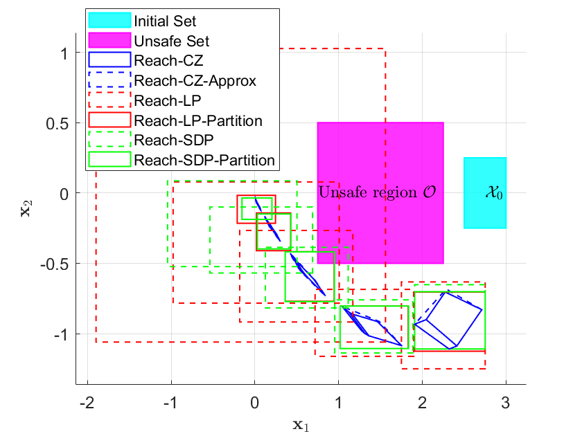
We denote the proposed exact reachability analysis method based on (7) and Theorem 1 as Reach-CZ and denote the over-approximation reachability analysis method based on (9) and Theorem 2 as Reach-CZ-Approx. We use the open-source Python toolboxes nn_robustness_analysis ([30]) to run the Reach-LP algorithm ([18]) and the Reach-SDP algorithm ([17]), and the versions with Greedy Sim-Guided Partition ([31]) for the initial sets, i.e., Reach-LP-Partition and Reach-SDP-Partition. All the parameters are kept as default. Table I summarizes the computation times and set over-approximation errors for the proposed method and other state-of-the-art methods including Reach-LP, Reach-LP-Partition, Reach-SDP, and Reach-SDP-Partition. The approximation errors are computed based on the difference ratio of sizes of over-approximated reachable sets and exact reachable sets at the last time step. Note that the proposed Reach-CZ method can return the exact reachable sets within a reasonable time. Note also that the proposed Reach-CZ-Approx method provides a better balance between efficiency and accuracy. Using about half the time consumed by Reach-LP-Partition, Reach-CZ-Approx achieves an approximation error that is over 20 times smaller than Reach-LP-Partition. Our constrained zonotope-based algorithms are implemented in Python with MOSEK [32]. All algorithms are tested in a computer with 3.7 GHz CPU and 32 GB memory.

Figure 3 illustrates reachable sets of the double integrator system using different methods. It can be observed that our method provides more accurate reachable sets for all the time steps compared with other methods. This is beneficial to avoid false unsafe detection in the safety verification problem; for example, with the unsafe region given in Figure 3, Reach-CZ and Reach-CZ-Approx can verify the safety of the neural feedback system while other methods can not.

Algorithm	Runtime [s]	Approx. Error
Reach-CZ (ours)	1.214	0
Reach-CZ-Approx (ours)	0.320	0.8
Reach-LP [18]	0.031	330
Reach-LP-Partition	0.891	19
Reach-SDP [17]	56.03	207
Reach-SDP-Partition	2048.89	11

TABLE I: Comparison of different reachability-based methods for the double integrator example. Reach-CZ returns exact reachable sets within a reasonable time. Compared with Reach-LP-Partition, Reach-CZ-Approx achieves over 20 times smaller errors using about half its time.

VI-B Nonlinear System Example

Consider the following discrete-time Duffing Oscillator model from [33]:

	$\displaystyle x_{1}(t+1)$	$\displaystyle=x_{1}(t)+0.3x_{2}(t)$
	$\displaystyle x_{2}(t+1)$	$\displaystyle=0.3x_{1}(t)+0.82x_{2}(t)-0.3[x_{1}(t)]^{3}+0.3u(t)$

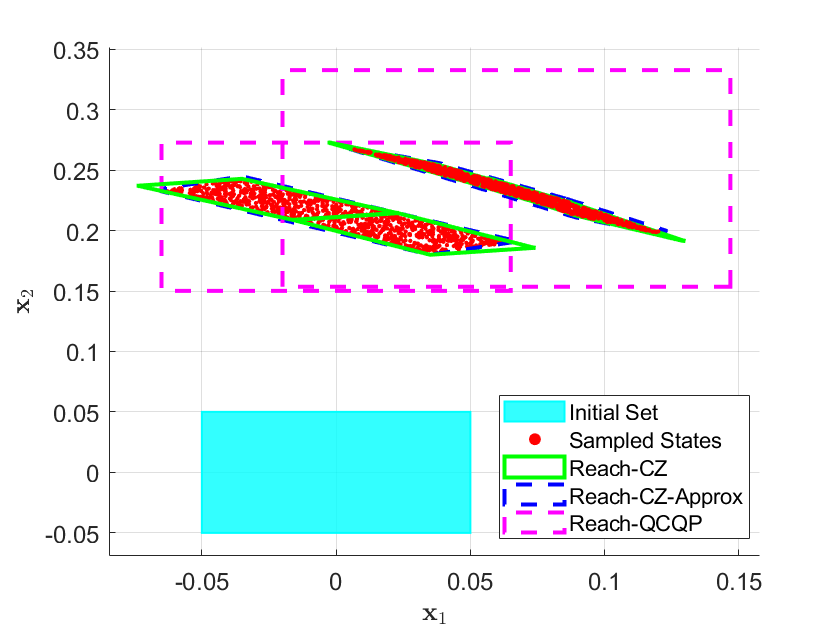
where $x_{1},x_{2}\in\mathbb{R}$ are the states and $u\in\mathbb{R}$ is the control input. We train an FNN controller to approximate the control law described in [33] and apply the algorithm based on Theorem 3 for $T=2$ time steps. Figure 4 shows the computed reachable sets and 1000 randomly generated sample trajectories. The sampled states are contained in the over-approximated reachable sets as expected. For comparison, we also apply the method based on quadratically constrained quadratic programming (QCQP) in [18], denoted as Reach-QCQP, to approximate the reachable sets for the Duffing Oscillator neural feedback system. Figure 4 indicates that although all the three methods only over-approximate the reachable sets, our constrained zonotope-based methods tend to have tiger bounds on the sampled states.

VII Conclusion

In this paper, we proposed a constrained zonotope-based method for analyzing the exact and over-approximated reachable sets of neural feedback systems. The exact reachable set of the neural feedback system is a union of constrained zonotopes and can be computed in a reasonable amount of time. The over-approximated method has much higher time efficiency than the exact method with a slight loss of accuracy. Based on the reachability analysis, we provided two LP-based conditions for safety verification of the neural feedback system. We also extended the proposed methods to a class of nonlinear systems. For future work, we plan to explore the tunability of constrained zonotopes to achieve a better trade-off between computational efficiency and approximating accuracy.

References

[1] F. Scarselli and A. C. Tsoi, “Universal approximation using feedforward neural networks: A survey of some existing methods, and some new results,” Neural Networks, vol. 11, no. 1, pp. 15–37, 1998.
[2] N. R. Pal and S. K. Pal, “A review on image segmentation techniques,” Pattern Recognition, vol. 26, no. 9, pp. 1277–1294, 1993.
[3] G. Hinton, L. Deng, D. Yu, G. E. Dahl, A.-r. Mohamed, N. Jaitly, A. Senior, V. Vanhoucke, P. Nguyen, T. N. Sainath, and B. Kingsbury, “Deep neural networks for acoustic modeling in speech recognition: The shared views of four research groups,” IEEE Signal Processing Magazine, vol. 29, no. 6, pp. 82–97, 2012.
[4] L. Shengbo, G. Yang, H. Lian, G. Hongbo, D. Jingliang, L. Shuang, W. Yu, C. Bo, L. Keqiang, R. Wei, and L. Jun, “Key technique of deep neural network and its applications in autonomous driving,” Journal of Automotive Safety and Energy, vol. 10, no. 2, p. 119, 2019.
[5] I. J. Goodfellow, J. Shlens, and C. Szegedy, “Explaining and harnessing adversarial examples,” arXiv preprint arXiv:1412.6572, 2014.
[6] G. Katz, C. Barrett, D. L. Dill, K. Julian, and M. J. Kochenderfer, “Reluplex: An efficient SMT solver for verifying deep neural networks,” in International Conference on Computer Aided Verification. Springer, 2017, pp. 97–117.
[7] S. Dutta, S. Jha, S. Sankaranarayanan, and A. Tiwari, “Output range analysis for deep feedforward neural networks,” in NASA Formal Methods Symposium. Springer, 2018, pp. 121–138.
[8] H.-D. Tran, P. Musau, D. M. Lopez, X. Yang, L. V. Nguyen, W. Xiang, and T. T. Johnson, “Parallelizable reachability analysis algorithms for feed-forward neural networks,” in IEEE/ACM 7th International Conference on Formal Methods in Software Engineering, 2019, pp. 51–60.
[9] J. A. Vincent and M. Schwager, “Reachable polyhedral marching (RPM): A safety verification algorithm for robotic systems with deep neural network components,” in IEEE International Conference on Robotics and Automation. IEEE, 2021, pp. 9029–9035.
[10] G. Singh, T. Gehr, M. Mirman, M. Püschel, and M. Vechev, “Fast and effective robustness certification,” Advances in Neural Information Processing Systems, vol. 31, 2018.
[11] L. K. Chung, A. Dai, D. Knowles, S. Kousik, and G. X. Gao, “Constrained feedforward neural network training via reachability analysis,” arXiv preprint arXiv:2107.07696, 2021.
[12] H.-D. Tran, D. Manzanas Lopez, P. Musau, X. Yang, L. V. Nguyen, W. Xiang, and T. T. Johnson, “Star-based reachability analysis of deep neural networks,” in International Symposium on Formal Methods. Springer, 2019, pp. 670–686.
[13] S. Dutta, X. Chen, and S. Sankaranarayanan, “Reachability analysis for neural feedback systems using regressive polynomial rule inference,” in Proceedings of the 22nd ACM International Conference on Hybrid Systems: Computation and Control, 2019, pp. 157–168.
[14] C. Huang, J. Fan, W. Li, X. Chen, and Q. Zhu, “ReachNN: Reachability analysis of neural-network controlled systems,” ACM Transactions on Embedded Computing Systems, vol. 18, no. 5s, pp. 1–22, 2019.
[15] W. Xiang, H.-D. Tran, X. Yang, and T. T. Johnson, “Reachable set estimation for neural network control systems: A simulation-guided approach,” IEEE Transactions on Neural Networks and Learning Systems, vol. 32, no. 5, pp. 1821–1830, 2020.
[16] R. Ivanov, J. Weimer, R. Alur, G. J. Pappas, and I. Lee, “Verisig: Verifying safety properties of hybrid systems with neural network controllers,” in Proceedings of the 22nd ACM International Conference on Hybrid Systems: Computation and Control, 2019, pp. 169–178.
[17] H. Hu, M. Fazlyab, M. Morari, and G. J. Pappas, “Reach-SDP: Reachability analysis of closed-loop systems with neural network controllers via semidefinite programming,” in IEEE 59th Conference on Decision and Control. IEEE, 2020, pp. 5929–5934.
[18] M. Everett, G. Habibi, C. Sun, and J. P. How, “Reachability analysis of neural feedback loops,” IEEE Access, vol. 9, pp. 163 938–163 953, 2021.
[19] A. Chakrabarty, C. Danielson, S. Di Cairano, and A. Raghunathan, “Active learning for estimating reachable sets for systems with unknown dynamics,” IEEE Transactions on Cybernetics, 2020.
[20] A. Devonport and M. Arcak, “Data-driven reachable set computation using adaptive Gaussian process classification and Monte Carlo methods,” in American Control Conference. IEEE, 2020, pp. 2629–2634.
[21] J. K. Scott, D. M. Raimondo, G. R. Marseglia, and R. D. Braatz, “Constrained zonotopes: A new tool for set-based estimation and fault detection,” Automatica, vol. 69, pp. 126–136, 2016.
[22] V. Raghuraman and J. P. Koeln, “Set operations and order reductions for constrained zonotopes,” Automatica, vol. 139, p. 110204, 2022.
[23] L. Jaulin, M. Kieffer, O. Didrit, and E. Walter, “Interval analysis,” in Applied Interval Analysis. Springer, 2001, pp. 11–43.
[24] R. E. Moore, R. B. Kearfott, and M. J. Cloud, Introduction to interval analysis. SIAM, 2009.
[25] B. S. Rego, G. V. Raffo, J. K. Scott, and D. M. Raimondo, “Guaranteed methods based on constrained zonotopes for set-valued state estimation of nonlinear discrete-time systems,” Automatica, vol. 111, p. 108614, 2020.
[26] M. Althoff, G. Frehse, and A. Girard, “Set propagation techniques for reachability analysis,” Annual Review of Control, Robotics, and Autonomous Systems, vol. 4, pp. 369–395, 2021.
[27] G. Singh, T. Gehr, M. Püschel, and M. Vechev, “An abstract domain for certifying neural networks,” Proceedings of the ACM on Programming Languages, vol. 3, no. POPL, pp. 1–30, 2019.
[28] B. S. Rego, J. K. Scott, D. M. Raimondo, and G. V. Raffo, “Set-valued state estimation of nonlinear discrete-time systems with nonlinear invariants based on constrained zonotopes,” Automatica, vol. 129, p. 109638, 2021.
[29] C. Sidrane, A. Maleki, A. Irfan, and M. J. Kochenderfer, “OVERT: An algorithm for safety verification of neural network control policies for nonlinear systems,” Journal of Machine Learning Research, vol. 23, no. 117, pp. 1–45, 2022.
[30] M. Everett and G. Habibi, “Robustness analysis tools,” https://github.com/mit-acl/nn_robustness_analysis.
[31] M. Everett, G. Habibi, and J. P. How, “Robustness analysis of neural networks via efficient partitioning with applications in control systems,” IEEE Control Systems Letters, vol. 5, no. 6, pp. 2114–2119, 2020.
[32] E. D. Andersen and K. D. Andersen, “The MOSEK interior point optimizer for linear programming: An implementation of the homogeneous algorithm,” in High Performance Optimization. Springer, 2000, pp. 197–232.
[33] T. Dang and R. Testylier, “Reachability analysis for polynomial dynamical systems using the Bernstein expansion.” Reliab. Comput., vol. 17, no. 2, pp. 128–152, 2012.