Dilepton production from chirally asymmetric matter
Abstract
We evaluate the dilepton production rate (DPR) from hot and dense chirally asymmetric quark matter. The presence of a finite chiral chemical potential (CCP) in the electromagnetic spectral function results in the appearance of new cut structures signifying additional scattering processes in the medium which leads to a significant enhancement in the DPR at lower values of invariant mass. The constituent quark mass evaluated using a 3-flavour Nambu–Jona-Lasinio model is also non-trivially affected by the CCP. These are found to result in a continuous dilepton production rate as a function of the invariant mass for higher values of temperature and baryonic chemical potential.
I Introduction
The study of QCD vacuum structure under extreme conditions of temperature and/or baryon density is one of the main objectives of relativistic heavy ion collision (HIC) experiments at RHIC and LHC. It is well established that the infinite number of energy-degenerate different vacuum configurations of QCD at zero and low temperatures can be characterised by topologically non-trivial gauge configurations with a non-zero winding number Shifman 1989. These gluon configurations are called instantons which can invoke transition between two different vacua by means of crossing a potential barrier with a height of the order of the QCD scale . This mechanism is known as instanton tunnelling Belavin et al. 1975; ’t Hooft 1976a; ’t Hooft 1976b. However, at high temperatures, for example, in the quark gluon plasma (QGP) phase of HICs, a copious production of another kind of gluon configuration, called sphalerons, is expected Manton 1983; Klinkhamer and Manton 1984. It is conjectured that the abundance of sphalerons can enhance the transition rate by crossing the barriers between different energy-degenerate vacua Kuzmin et al. 1985; Arnold and McLerran 1987; Khlebnikov and Shaposhnikov 1988; Arnold and McLerran 1988. The topologically non-trivial guage field configurations can switch the helicities of quarks while interacting with them. This in turn leads to the breaking of parity () and charge-parity () symmetries by creating an asymmetry between left and right handed quarks via the axial anomaly of QCD Adler 1969; Bell and Jackiw 1969. Chirality imbalance can be produced locally as there is no direct observation of the violation of and in QCD globally Adler 1969; Bell and Jackiw 1969; McLerran et al. 1991; Moore and Tassler 2011. This locally induced chirality imbalance is characterised by means of a chiral chemical potential (CCP) which basically represents the difference between the number of right and left-handed quarks.
HICs with a non-zero impact parameter can give rise to very high magnetic fields of the order of few Kharzeev et al. 2008; Skokov et al. 2009. Such high magnetic fields in presence of chirality imbalance can lead to a separation of positive and negative charges with respect to the reaction plane and induce a current along the magnetic field dubbed as chiral magnetic effect (CME) Fukushima et al. 2008; Kharzeev et al. 2008; Kharzeev and Warringa 2009; Bali et al. 2012. Substantial efforts have been made to detect CME in HIC experiments at the RHIC at Brookhaven. Very recently, the STAR Collaboration has performed an extensive analysis which has provided no indication of CME in HICs Abdallah et al. 2021. As a consequence, new techniques for experimental determination of CME have been proposed An et al. 2022; Milton et al. 2021.
Since a local domain of chirality imbalance is expected to be produced in QGP, in addition to the CME there have been intense studies on the phase structure Ruggieri and Peng 2016; Ruggieri et al. 2016; Ruggieri et al. 2020, microscopic transport phenomena Vilenkin 1979; Vilenkin 1980; Fukushima et al. 2008; Son and Surowka 2009, collective oscillations Akamatsu and Yamamoto 2013; Carignano and Manuel 2019; Carignano and Manuel 2021, fermion damping rate Carignano and Buballa 2020 and collisional energy loss of fermions Carignano and Manuel 2021 as well as properties of electromagnatic spectral function Ghosh et al. 2022 in chirally imbalanced medium. Moreover, chirally asymmetric plasma is expected to be produced in the gap regions of the magnetospheres of pulsars and black holes Gorbar and Shovkovy 2021 and other stellar astrophysical scenario Charbonneau and Zhitnitsky 2010; Akamatsu and Yamamoto 2013; Kaminski et al. 2016; Yamamoto 2016; Shovkovy 2021. Furthermore, it is worthwhile to mention that CME has indeed been observed in condensed matter systems particularly in 3D Dirac as well as Weyl semimetals Li et al. 2016; Li and Kharzeev 2016; Kharzeev 2014; Kharzeev et al. 2016; Huang 2016; Landsteiner 2016; Gorbar et al. 2018; Joyce and Shaposhnikov 1997; Tashiro et al. 2012. Thus the study of the properties of chirally imbalanced matter continues to be a matter of major topical interest.
It is well known that the hot and dense matter produced in HICs cools via rapid expansion under its own pressure passing through different stages of evolution. However, the whole process is very transient (few fm/c) restricting the possibility of a direct observation. So to investigate microscopic as well as bulk properties of QGP one has to rely on indirect probes and observables Wong 1995. Electromagnetic probes, photons and dileptons have long been used as reliable probes of HICs. Because they participate only in electromagnetic interaction, their mean free paths are much larger than the typical size of the system. As a consequence, once produced they tend to leave the system without suffering further interactions, thus carrying unaltered information about the space-time region from where they are produced McLerran and Toimela 1985; Kajantie et al. 1986; Weldon 1990; Alam et al. 1996; Alam et al. 2001; Rapp and Wambach 2000; Aurenche et al. 2000; Arnold et al. 2001; Rapp and van Hees 2010; Chatterjee et al. 2010; Sarkar and Ghosh 2012. As the production rate of dileptons and photons is directly proportional to the electromagnetic spectral function, the study of its analytic properties is of central importance Mallik and Sarkar 2016; Wong 1995; Alam et al. 2001; Sarkar and Ghosh 2012. Such a study in chirally imbalanced hot and/or dense matter has recently been performed in Ghosh et al. 2022 where a rich cut-structure was revealed. The step-like structure of the spectral function observed in certain invariant mass range were attributed to the thresholds of Unitary and Landau cuts indicating additional scattering processes in the medium. We expect that such structures will have non-trivial effects on the dilepton spectrum.
The imaginary part of the electromagnetic current correlator containing the modified quark propagators in the presence of a hot and dense medium is the most important component in the evaluation of the dilepton production rate (DPR) which determines the thresholds as well as the intensity of emission of dileptons Alam et al. 1996; Alam et al. 2001. Thus it has a crucial dependence in the value of quark mass. As the system cools, the quark condensate builds up due to the breaking of chiral symmetry which results in a large value of the quark mass ( few hundred MeV). The non-perturbative nature of QCD at low energies severely hinders the theoretical analysis of these phenomena using first principle calculations. As an alternative, we have used the Nambu–Jona-Lasinio (NJL) model Nambu and Jona-Lasinio 1961a; Nambu and Jona-Lasinio 1961b which is built by respecting the global symmetries of QCD, most importantly the chiral symmetry Klevansky 1992; Buballa 2005; Vogl and Weise 1991. This model has been very useful to probe the vacuum structure of QCD at arbitrary values of temperature, baryon chemical potential (BCP) and CCP Ruggieri 2011; Fukushima et al. 2010; Farias et al. 2016; Chao et al. 2013; Yu et al. 2014; Yu et al. 2016; Chaudhuri et al. 2021a.
In this work, we shall evaluate the dilepton production rate (DPR) from a (locally) chirally imbalanced quark matter expected to be produced in relativistic HIC experiments. We use the 3-flavor NJL model to evaluate the constituent quark mass by solving the self-consistent gap equations. The quark mass for different flavours will go as an input in the electromagnetic spectral function. We have made use of the analytic structure of the in-medium spectral function to obtain the thresholds of dilepton production due to various scattering processes involving quarks for both zero and non-zero values of .
The paper is organized as follows. In the next section we discuss the formulation of the dilepton production rate at zero and finite value of the CCP. Next, we discuss in Section III the evaluation of the constituent quark mass from a 3-flavour NJL model. Section IV deals with the numerical results followed by a summary and discussion in Section V.
II DILEPTON PRODUCTION RATE
In QGP, a quark can interact with an anti-quark to produce a virtual photon, which subsequently decays into a lepton and anti-lepton pair (see Fig. 1).

The dilepton production rate (DPR) from a hot and dense medium is already calculated in Refs. McLerran and Toimela 1985; Weldon 1990; Wong 1995; Mallik and Sarkar 2016; Bandyopadhyay and Mallik 2017; Ghosh and Chandra 2018. But, for the sake of completeness, we will briefly demonstrate few important steps. First, we consider an initial state of a quark/antiquark with momentum moving towards to a final state consisting a quark/antiquark of momentum plus a pair of leptons of momenta and respectively. The probability amplitude for such a transition is , where is the scattering matrix expressed as
| (1) |
in which is the time-ordering operator and
| (2) |
is the Lagrangian (density) for local interaction. Our choice of metric tensor is . In the above equation, the conserved vector currents corresponding to the leptons and quarks denoted by and respectively, are coupled to the photon field represented by . It can be shown that, the first non-trivial contribution to the above mentioned process comes from the second order term in the matrix expansion and the expression of the squared amplitude is given by,
| (3) |
Now the dilepton multiplicity from thermal QGP medium is expressed as Mallik and Sarkar 2016
| (4) |
where is the partition function of the system and the summation signifies sum over all leptonic spin configurations. Using Eq. (3) in Eq. (4) and after some simplifications, we arrive at Ghosh and Chandra 2018
| (5) |
where,
| (6) | |||||
| (7) |
Here represents the ensemble average and is the total momentum of the lepton-pair. So the dilepton production rate (DPR) becomes
| (8) |
Now to calculate DPR in presence of a medium it is useful to write both the and in terms of time ordered correlation functions so that one can apply the real time formulation of finite temperature field theory Mallik and Sarkar 2016; Ghosh and Chandra 2018; Ghosh et al. 2020; Chaudhuri et al. 2021b. Thus we get
| (9) |
Till now we have not specified any explicit form of the currents and which are required to evaluate the quantities and . In this work, we have considered
| (10) | |||||
| (11) |
where, represents -flavor quark field multiplet with corresponding charge matrix , is the lepton field and is the absolute value of the electric charge of an electron. Using Eqs. (10) and (11) it can be shown that
| (12) | |||||
| (13) |
where the trace over Dirac, flavor and color spaces are indicated by the subscript ‘d’, ‘f’, and ‘c’ respectively; is the 11-component of the real time quark propagator and is the vacuum propagator for leptons with Feynman boundary condition which is expressed as
| (14) |
with being the mass of the lepton. It is to be noted that, in Eq. (12), the quark propagator is diagonal in both the flavor and color space i.e.
| (15) |
Since both the currents and are conserved: , consequently the matter tensor as well as the leptonic tensor are transverse to the momentum i.e.
| (16) |
These transversality conditions enforce the following Lorentz structure of :
| (17) |
Putting this back in Eq. (9), and using the transversality condition for matter tensor we get the DPR as
| (18) |
It is easy to check, by substituting Eq. (14) into Eq. (13), that
| (19) |
The effects of finiteness of CCP will be encoded in the matter tensor part of Eq. (18). Thus we shall consider the following two cases.
II.1 DPR at
To evaluate matter part at finite temperature for vanishing values of CCP, one requires the 11-component of the real time thermal quark propagator. In the spectral representation this can be expressed as Mallik and Sarkar 2016
| (20) |
where, is the fermionic spectral function with being the constituent mass of a quark with flavour and is the distribution like function containing the true Fermi-Dirac thermal distributions of the quarks given by
| (21) |
in which is the BCP. Now in the local rest frame (LRF) of the medium, using Eqs. (20), (21) and (15) in Eq. (12) one gets after some algebra
| (22) | |||||
where, , , and . Note that, the first delta function appearing in Eq. (22), termed as the unitary-I cut, represents to the contribution from quark-antiquark annihilation to a positive energy time-like virtual photon (and the corresponding time reversed process where such a photon decays into a quark-antiquark pair). The delta function in the second term (the unitary-II cut) corresponds to similar process but the virtual photon is of negative energy. The last two delta functions are called the Landau cuts, which are purely medium dependent contributions, stand for the scattering/emission processes such as absorption of a space-like virtual photon by a quark/antiquark and the consequent time reversed processes. It can be easily checked that, the contributions from unitary-I and unitary-II cuts are non-zero in the kinematic regions and respectively.

On the other hand, the kinematic domain for both the Landau cuts is in the space-like region . This cut structure of in the complex -plane is depicted in Fig. 2. Since, we are interested in the physical dileptons with positive energy and time-like four momentum i.e and , it follows that, only the unitary-I cut contributions are kinematically allowed. It should be noted that, the kinematic domains are directly related to constituent quark mass and hence can be different for different flavors Ghosh and Chandra 2018; Ghosh et al. 2020; Chaudhuri et al. 2021b. Now, with the physical restrictions previously mentioned, the integral of Eq. (22) can be evaluated analytically (the integral has been performed using the Dirac delta functions present in the integrand and the integral trivially gives a factor of ). Using this result in Eq. (18), we finally arrive at the following analytical expression for the DPR at vanishing CCP Ghosh and Chandra 2018; Greiner et al. 2011
| (23) | |||||
where . The step functions in the above expression restrict the production of dileptons with invariant mass and .
II.2 DPR at
This subsection is devoted to the evaluation of in a medium in presence of chiral imbalance. Here, one needs the 11-component of the real time thermal quark propagator with finite values of CCP. In the spectral representation the later can be expressed as Mallik and Sarkar 2016; Ghosh et al. 2022
| (24) | |||||
where the fermionic spectral function in presence of CCP is
| (25) |
in which, with corresponds to the helicity of the propagating Fermion and contains the complicated Dirac structure as
| (26) |
In the above equation, , and is already defined in Eq. (21). Using this we get
| (27) | |||||
with . Now contracting with the metric tensor and concentrating on the imaginary part we get
| (28) | |||||
where,
| (29) | |||||
Here, some discussions related to the analytic structure of in the complex plane are in order. It can be seen that, in presence of finite , the imaginary part of the matter tensor consists of sixteen Dirac delta functions which leads to several branch cuts in the complex plane. The terms containing and are referred to as Unitary-I and Unitary-II cuts respectively as already mentioned in the previous section. However, in non-zero CCP case each of the Unitary cut consists of further sub-cuts owing to the different helicities . These different cuts correspond to different physical processes. For example, the Unitary-I (Unitary-II) cuts represent the decay of a virtual photon having positive (negative) energy to real quark-antiquark pair (and the corresponding time reversed process). The terms with the remaining two delta functions, i.e. and , are called Landau-I and Landau-II cuts which also contain four sub-cuts corresponding to distinct helicities. As already mentioned, Landau cuts stand for the emission(absorption) processes in which a real quark/antiquark in the thermal medium emits (absorbs) a virtual photon. The detailed analysis to find out respective kinematic domains such that the imaginary part of receives non-trivial contributions from the sixteen different delta function has been done in Ghosh et al. 2022. Here we only quote the final result in tabular form in Eq. (II.2).
The pictorial representation of the complex analytical structure of expressed in Eq. (II.2) is shown in Fig. 3. Since we are interested in physical dileptons, we will restrict ourselves to the time-like kinematic domains with and . Form Fig. 3 it is evident, in addition to the Unitary-I cut, some portion of the Landau cuts will also contribute to the and hence to the DPR. This contribution at lower invariant mass region is purely a finite CCP effect. Moreover, notice that, the thresholds of the Unitary cuts strongly depend on and . Consequently, for , a positive energy photon with can in principle decay into a real quark-antiquark pair below the usual threshold of pair production ; even for a space-like photon. Finally, for sufficiently high , the forbidden gap between the Unitary and Landau cut contributions will vanish irrespective of the value of which enables the production of a continuous spectrum of dileptons through out the whole range of invariant mass, which is again possible only in a chirally asymmetric medium.

Now, substituting Eqs. (19) and (28) in Eq. (18) we get
| (49) | |||||
In Eq. (49), the angular integral is performed using the Dirac delta functions present in the integrand and the azimuthal integral gives a factor of . However, unlike the vanishing CCP case, here the analytical evaluation of the remaining integral becomes cumbersome and hence will be evaluated numerically to obtain the DPR. Note that, while calculating DPR the constituent quark mass () for different flavour, which depends on the external parameters, such as, temperature, BCP and CCP, are required. Here NJL model is used to calculate in different physical conditions.
III THE CONSTITUENT QUARK MASS using 3-flavor Nambu-Jona–Lasinio MODEL
In this section we briefly outline few important steps to calculate constituent quark mass using NJL model. The Lagrangian for the 3-flavor gauged NJL model is given by
| (50) | |||||
In the above expression, is the quark field multiplet with three flavors () and three colors () (flavour and colour indices are suppressed). is the current quark mass matrix. s are the Gell-Mann matrices corresponding to the flavor . The isospin symmetry on the Lagrangian level is assumed, i.e., , while -symmetry is explicitly broken, so that . is the the scalar coupling strength and the term represents the six-point Kobayashi-Maskawa-t’Hooft (KMT) interaction which is responsible for breaking of the axial symmetry Klevansky 1992. Using mean field approximation one arrives at the following gap equations:
| (51) | |||||
| (52) | |||||
| (53) |
where
| (54) |
The self-consistent solution of Eqs. (51)–(53) results in and/or dependence of for different values of CCP. Notice that, the medium independent integral Eq. (54) is ultraviolet divergent. Since the NJL Lagragian is known to be non-renormalizable owing to the point-like interaction between the quarks Klevansky 1992, one has to specify a proper regularization scheme.
To avoid a cutoff artifact, several smooth regularization procedure has been used in the literature by introducing a form factor in the diverging vacuum integrals. One can choose different functional form of this , such as, the Lorentzian type form factors Fukushima et al. 2010; Gatto and Ruggieri 2010; Gatto and Ruggieri 2011; Gatto and Ruggieri 2013; Ghosh et al. 2022; Yu et al. 2014 and Woods-Saxon type form factors Fayazbakhsh and Sadooghi 2011; Fayazbakhsh et al. 2012; Fayazbakhsh and Sadooghi 2014. In this work, we have used first kind of smoothing function by introducing a multiplicative form factor Fukushima et al. 2010; Yu et al. 2015; Ghosh et al. 2022
| (55) |
In the limit the form factor is reduced to the sharp cutoff function which infer that for larger values of , the cutoff artifacts are expected to increase. On the other hand, for small values, it is impossible to fit different phenomenological values, such as, pion decay constant, the vacuum value of chiral condensate etc Gatto and Ruggieri 2011. Here, we have taken for numerical convenience. The other model parameters are given in Table 1.
| (MeV) | (MeV) | (MeV) | ||
These parameters are determined by fitting , , , and to their phenomenological values Yu et al. 2015.
IV Numerical Results

In this section, we present the numerical results for constituent quark masses of different flavors which are the main inputs while calculating the DPR from a chirally asymmetric hot and dense medium. In Fig. 4, we have shown the variation of constituent mass of ’up’ and ’strange’ quarks as a function of temperature for different values of BCP and CCP which are evaluated by solving Eqs. (51)-(53) self-consistently. One can observe that, the spontaneous breaking of the chiral symmetry at small values of temperature results in large values of constituent mass for both ‘up’ and ‘strange’ quarks owing to the large values of quark condensate for all the cases. Now, as the temperature is increased, the constituent mass of the low lying quarks remains constant upto a certain value of temperature, then falls off sharply in a small range of temperature and finally becomes nearly equal to the bare masses of the quarks at high values representing the pseudo-chiral phase transition due to the (partial) restoration of the chiral symmetry. However, the strange quark mass decreases smoothly when compared to that of the up quark and it can be seen that even at MeV the s-quark mass is still substantially higher than its current mass. The explanation of this behaviour comes from Eq. (54). As the current quark mass becomes large, the excitation probability of the quark-antiquark pair becomes thermally suppressed, which leads to a small -dependence of when compared to the low lying quarks Hatsuda and Kunihiro 1987. Now at high temperature as the condensates of and -quarks melt, the third term of Eq. (53) becomes negligible and the constituent mass of strange quark is solely determined by the condensate resulting in a smooth variation of . This indicates that symmetry is not even a good approximate symmetry at temperatures larger than 200 MeV which may be due to the fact that the restoration of the chiral symmetry in the different quark sectors is achieved quite differently Hatsuda and Kunihiro 1994. Now for finite values of BCP, it is seen that the qualitative behaviour of the -dependence of the u and s-quark masses remain same, although the transition temperature is found to decrease thus mimicking the conjectured QCD phase diagram. In presence of finite CCP, the constituent mass of both u and s-quarks are found to increase in the low temperature region indicating an enhancement in the magnitude of the quark condensate at small values of . However, the transition from chirality broken to the restored phase occurs at relatively smaller values of temperature which shows that, at high values of temperature, the formation of quark condensate is hindered by the presence of finite , an exact opposite result compared to the low temperature values. These phenomena can be termed as ‘chiral catalysis’ and ‘inverse chiral catalysis’ respectively Ghosh et al. 2022.


Next, we present the numerical results for DPR from a hot and dense medium in presence of chiral imbalance. Note that, all the results shown hereafter are obtained ignoring the lepton mass i.e. and considering the momentum MeV. In Fig. 5(a) we have depicted DPRs as a function of invariant mass at MeV and for different values of CCP. The DPR at (black solid line) is also shown for comparison. For case, DPR is restricted to low values of invariant mass as already discussed in Sec. II.1. The non-trivial contributions starts from just below MeV owing to the Unitary-I cut threshold . Now from Fig. 4 one can observe that, constituent mass of u-quark at MeV is MeV. This explains the behaviour in case of vanishing CCP. However, in case of MeV a significant enhancement in the DPR can be seen owing to non-trivial Landau cut contributions. From Eq. (II.2), one can observe that, the Landau cut contribution will be finite for physical dileptons when . This can be rewritten as . For MeV, GeV. So around that value of invariant mass the Landau cut contribution should end, which can be seen in Fig. 5(a) (solid red line). Moreover, the unitary cut contributions starts at a lower value of invariant mass than case although the constituent mass is higher due to presence of finte CCP. To understand this let us concentrate on the Unitary cut thresholds for production of physical dileptons. From Eq. (II.2), this is expressed as , which can be simplified further to arrive at . At MeV, the constituent mass of the u-quark is MeV. So for MeV, the Unitary cut contribution starts at GeV, which is evident from Fig. 5(a). This indicates that a chirally asymmetric medium can induce pair production at comparatively lower values of invariant mass as discussed in Sec. II.2. It also explains the forbidden gap between Landau and Unitary cut where dilepton production ceases to occur. Now, from the above two discussions about the kinematic domain of Landau (Unitary) cut, it is clear that as we increase the threshold for dilepton production move towards higher (lower) values of invariant mass. Consequently, for higher values of CCP i.e. and MeV, the Unitary and Landau cut contributions merge with each other resulting a continuous spectrum of dileptons for the whole range of invariant mass. In Fig. 5(b) we have presented DPRs as a function of invariant mass at MeV considering a finite baryon density ( MeV) for four different values of . Notice that, for MeV plot (solid red line) the Landau cut threshold ends at the same value as in zero baryon density case. This is understandable from the fact that the Landau cut threshold only depends on . However, the Unitary cut threshold, which is directly related to the constituent mass of quarks move towards lower values of invariant mass. This can be explained from Fig. 4 where one can observe that for finite values of the (pseudo) chiral transition temperature moves towards the lower values of , resulting in a decrease in the magnitude of . In Fig. 5(b), we find a continuous dilepton spectrum for higher values of which can be understood in a similar fashion as discussed earlier. In Fig. 5(c), we have considered an even higher baryon density ( MeV) keeping all the other parameters same as Figs. 5(a) and (b). From the plot of vanishing CCP case, it is evident that, constituent mass of low lying quarks have decreased further such that, the Unitary cut threshold for is already below the Landau cut threshold for MeV. As a consequence, we get a continuous spectrum of dileptons for the whole range of invariant mass for all values of CCP shown in the figure.
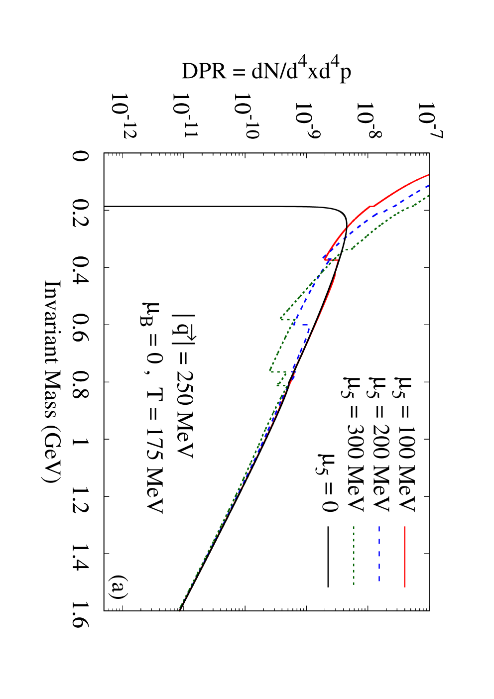
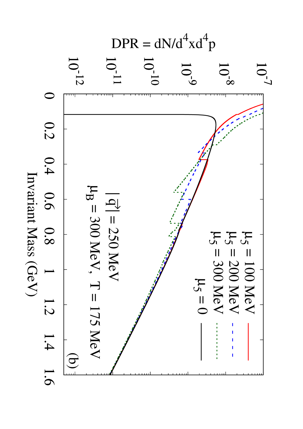
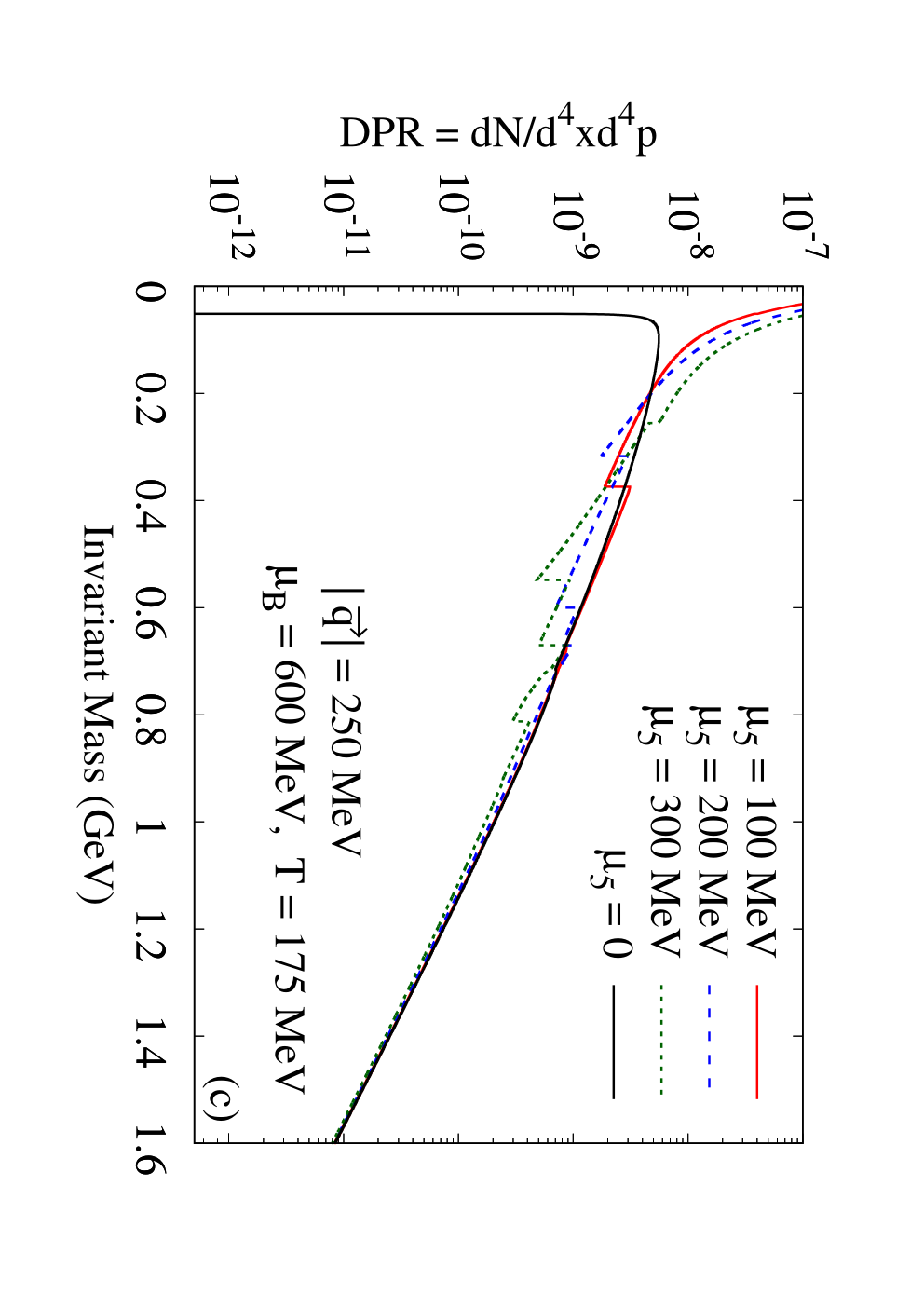


In Figs. 6(a), (b) and (c) we have depicted DPRs as a function of invariant mass at MeV for different values of CCP for and 600 MeV respectively. Considering the zero baryon density case (Fig. 6(a)), it can be seen that, the Unitary cut threshold for is already below the Landau cut threshold for MeV (note that, since the Landau cut contribution only depends of , it will be same as the previous case). Moreover, from Fig. 4, it is clear that, at MeV, the constituent mass of low lying quarks are always below MeV. As a result, at MeV, for all finite case shown in the figure, the Landau and Unitary cut contribution will merge and a continuous spectrum of dilepton will emerge as evident from Figs. 6 (a), (b) and (c).
A similar trend is visible in Figs. 7(a), (b) and (c) where the DPR is plotted for MeV. Here, because of restoration of chiral symmetry the constituent mass of the low lying quarks goes to the bare mass limit (see Fig. 4). Consequently, the threshold of unitary cut starts at smaller values of the invariant mass. Moreover, since the temperature considered in this case is higher than all the previous cases the increase in thermal phase space results in a significant enhancement in the overall magnitude of DPRs when compared to Figs. 5(a), (b) and (c)) Ghosh and Chandra 2018; Ghosh et al. 2020; Chaudhuri et al. 2021b.
We end this section with a discussion on the experimental observation of the effects of chiral imbalance on the dilepton spectra. Keeping in mind that dileptons are emitted at all stages of the collision, the DPR from quark matter as well as those from and decays and other hadronic reactions have to be evolved in space-time using (1+3)d hydrodynamics (with ). As discussed earlier, chiral imbalance may be created in HICs locally which leads to a continuous spectrum with a distinct shape in the low invariant mass region of the DPR from quark matter. It should be noted that the creation of a local domain with chiral imbalance changes from event to event and the event average value of any -dependent observable is zero. Thus, the analysis must be done on an event by event basis. Now let us consider an event in which a domain with chirally imbalanced quark matter is created. Due to the hydrodynamic expansion it will cool and undergo a transition to hadronic matter which presumably will also be in and odd phase. If that be the case, there will be effect of chiral imbalance on the DPR coming from resonance decay and hadronic reactions as well. Andrianov et. al. Andrianov et al. 2012 have predicted that such matter will produce an excess of dileptons in the resonance region. Together with the enhancement of DPR from quark matter in the low invariant mass region (i.e. non-zero yield in the invariant mass range GeV with MeV or higher) seen in this work, the total dilepton yield could explain the observed low mass enhancement seen in the PHENIX experiment Liao 2015 for central collisions which cannot be explained by invoking the temperature and density dependent medium modifications of hadronic spectral functions alone.
V SUMMARY & CONCLUSION
In this work we studied the dilepton production rate from hot and dense chirally asymmeteric matter likely to be produced in relativistic HICs. The electromagnetic spectral function which is the principal component in the DPR is found to be modified due to the presence of a CCP. The constituent quark mass which appears in the in-medium propagator is evaluated in a self-consistent manner using a 3-flavour NJL model and is also non-trivially affected by the CCP. Specifically, in presence of the quark condensate is found to be enhanced at small values of while it is hindered at high values of temperature. We have also analyzed the complete analytic structure of the spectral function of the chirality imbalanced medium in the complex energy plane and have found a nontrivial Landau cut in the physical kinematic region signifying additional scattering processes in the medium; a purely finite CCP effect. As a consequence the DPR acquires contributions from both the unitary and Landau cuts for production of dileptons with positive energy and time-like four momentum. Owing to the emergence of the Landau cut the DPR is highly enhanced in the low invariant mass region compared to the case with a vanishing CCP. It is also found that the Landau cut threshold is independent of the constituent quarks mass though the unitary cut threshold has a non-trivial dependence on both and . For small values of and a forbidden gap exists between Unitary and Landau cuts where production of dileptons is kinematically restricted. However, as we increase the CCP at fixed values of and the Landau cut threshold moves towards higher invariant mass. As a result the forbidden gap keeps shrinking and eventually merges with each other producing a continuous spectrum of dileptons as a function of invariant mass even for small values of temperature where chiral symmetry is still broken. For higher values of temperature and/or BCP the forbidden gap completely disappears and a significant rise in dilepton production rate is observed owing to the availability of larger thermal phase space.
Acknowledgments
NC, SS and PR are funded by the Department of Atomic Energy (DAE), Government of India. SG is funded by the Department of Higher Education, Government of West Bengal, India.
References
- Shifman (1989) M. A. Shifman, Sov. Phys. Usp. 32, 289 (1989).
- Belavin et al. (1975) A. A. Belavin, A. M. Polyakov, A. S. Schwartz, and Y. S. Tyupkin, Phys. Lett. B 59, 85 (1975).
- ’t Hooft (1976a) G. ’t Hooft, Phys. Rev. Lett. 37, 8 (1976a).
- ’t Hooft (1976b) G. ’t Hooft, Phys. Rev. D 14, 3432 (1976b), [Erratum: Phys.Rev.D 18, 2199 (1978)].
- Manton (1983) N. S. Manton, Phys. Rev. D 28, 2019 (1983).
- Klinkhamer and Manton (1984) F. R. Klinkhamer and N. S. Manton, Phys. Rev. D 30, 2212 (1984).
- Kuzmin et al. (1985) V. A. Kuzmin, V. A. Rubakov, and M. E. Shaposhnikov, Phys. Lett. B 155, 36 (1985).
- Arnold and McLerran (1987) P. B. Arnold and L. D. McLerran, Phys. Rev. D 36, 581 (1987).
- Khlebnikov and Shaposhnikov (1988) S. Y. Khlebnikov and M. E. Shaposhnikov, Nucl. Phys. B 308, 885 (1988).
- Arnold and McLerran (1988) P. B. Arnold and L. D. McLerran, Phys. Rev. D 37, 1020 (1988).
- Adler (1969) S. L. Adler, Phys. Rev. 177, 2426 (1969).
- Bell and Jackiw (1969) J. S. Bell and R. Jackiw, Nuovo Cim. A 60, 47 (1969).
- McLerran et al. (1991) L. D. McLerran, E. Mottola, and M. E. Shaposhnikov, Phys. Rev. D 43, 2027 (1991).
- Moore and Tassler (2011) G. D. Moore and M. Tassler, JHEP 02, 105 (2011), arXiv:1011.1167 [hep-ph] .
- Kharzeev et al. (2008) D. E. Kharzeev, L. D. McLerran, and H. J. Warringa, Nucl. Phys. A803, 227 (2008), arXiv:0711.0950 [hep-ph] .
- Skokov et al. (2009) V. Skokov, A. Yu. Illarionov, and V. Toneev, Int. J. Mod. Phys. A24, 5925 (2009), arXiv:0907.1396 [nucl-th] .
- Fukushima et al. (2008) K. Fukushima, D. E. Kharzeev, and H. J. Warringa, Phys. Rev. D78, 074033 (2008), arXiv:0808.3382 [hep-ph] .
- Kharzeev and Warringa (2009) D. E. Kharzeev and H. J. Warringa, Phys. Rev. D 80, 034028 (2009), arXiv:0907.5007 [hep-ph] .
- Bali et al. (2012) G. S. Bali, F. Bruckmann, G. Endrodi, Z. Fodor, S. D. Katz, S. Krieg, A. Schafer, and K. K. Szabo, JHEP 02, 044 (2012), arXiv:1111.4956 [hep-lat] .
- Abdallah et al. (2021) M. Abdallah et al. (STAR), (2021), arXiv:2109.00131 [nucl-ex] .
- An et al. (2022) X. An et al., Nucl. Phys. A 1017, 122343 (2022), arXiv:2108.13867 [nucl-th] .
- Milton et al. (2021) R. Milton, G. Wang, M. Sergeeva, S. Shi, J. Liao, and H. Z. Huang, Phys. Rev. C 104, 064906 (2021), arXiv:2110.01435 [nucl-th] .
- Ruggieri and Peng (2016) M. Ruggieri and G. X. Peng, Phys. Rev. D 93, 094021 (2016), arXiv:1602.08994 [hep-ph] .
- Ruggieri et al. (2016) M. Ruggieri, G. X. Peng, and M. Chernodub, Phys. Rev. D 94, 054011 (2016), arXiv:1606.03287 [hep-ph] .
- Ruggieri et al. (2020) M. Ruggieri, M. N. Chernodub, and Z.-Y. Lu, Phys. Rev. D 102, 014031 (2020), arXiv:2004.09393 [hep-ph] .
- Vilenkin (1979) A. Vilenkin, Phys. Rev. D 20, 1807 (1979).
- Vilenkin (1980) A. Vilenkin, Phys. Rev. D 22, 3080 (1980).
- Son and Surowka (2009) D. T. Son and P. Surowka, Phys. Rev. Lett. 103, 191601 (2009), arXiv:0906.5044 [hep-th] .
- Akamatsu and Yamamoto (2013) Y. Akamatsu and N. Yamamoto, Phys. Rev. Lett. 111, 052002 (2013), arXiv:1302.2125 [nucl-th] .
- Carignano and Manuel (2019) S. Carignano and C. Manuel, Phys. Rev. D 99, 096022 (2019), arXiv:1811.06394 [hep-ph] .
- Carignano and Manuel (2021) S. Carignano and C. Manuel, Phys. Rev. D 103, 116002 (2021), arXiv:2103.02491 [hep-ph] .
- Carignano and Buballa (2020) S. Carignano and M. Buballa, Phys. Rev. D 101, 014026 (2020), arXiv:1910.03604 [hep-ph] .
- Ghosh et al. (2022) S. Ghosh, N. Chaudhuri, S. Sarkar, and P. Roy, (2022), arXiv:2201.06473 [hep-ph] .
- Gorbar and Shovkovy (2021) E. V. Gorbar and I. A. Shovkovy, (2021), arXiv:2110.11380 [astro-ph.HE] .
- Charbonneau and Zhitnitsky (2010) J. Charbonneau and A. Zhitnitsky, JCAP 08, 010 (2010), arXiv:0903.4450 [astro-ph.HE] .
- Kaminski et al. (2016) M. Kaminski, C. F. Uhlemann, M. Bleicher, and J. Schaffner-Bielich, Phys. Lett. B 760, 170 (2016), arXiv:1410.3833 [nucl-th] .
- Yamamoto (2016) N. Yamamoto, Phys. Rev. D 93, 065017 (2016), arXiv:1511.00933 [astro-ph.HE] .
- Shovkovy (2021) I. A. Shovkovy, (2021), arXiv:2111.11416 [nucl-th] .
- Li et al. (2016) Q. Li, D. E. Kharzeev, C. Zhang, Y. Huang, I. Pletikosic, A. V. Fedorov, R. D. Zhong, J. A. Schneeloch, G. D. Gu, and T. Valla, Nature Phys. 12, 550 (2016), arXiv:1412.6543 [cond-mat.str-el] .
- Li and Kharzeev (2016) Q. Li and D. E. Kharzeev, Nucl. Phys. A 956, 107 (2016).
- Kharzeev (2014) D. E. Kharzeev, Prog. Part. Nucl. Phys. 75, 133 (2014), arXiv:1312.3348 [hep-ph] .
- Kharzeev et al. (2016) D. E. Kharzeev, J. Liao, S. A. Voloshin, and G. Wang, Prog. Part. Nucl. Phys. 88, 1 (2016), arXiv:1511.04050 [hep-ph] .
- Huang (2016) X.-G. Huang, Rept. Prog. Phys. 79, 076302 (2016), arXiv:1509.04073 [nucl-th] .
- Landsteiner (2016) K. Landsteiner, Acta Phys. Polon. B 47, 2617 (2016), arXiv:1610.04413 [hep-th] .
- Gorbar et al. (2018) E. V. Gorbar, V. A. Miransky, I. A. Shovkovy, and P. O. Sukhachov, Low Temp. Phys. 44, 487 (2018), arXiv:1712.08947 [cond-mat.mes-hall] .
- Joyce and Shaposhnikov (1997) M. Joyce and M. E. Shaposhnikov, Phys. Rev. Lett. 79, 1193 (1997), arXiv:astro-ph/9703005 .
- Tashiro et al. (2012) H. Tashiro, T. Vachaspati, and A. Vilenkin, Phys. Rev. D 86, 105033 (2012), arXiv:1206.5549 [astro-ph.CO] .
- Wong (1995) C. Y. Wong, Introduction to high-energy heavy ion collisions (1995).
- McLerran and Toimela (1985) L. D. McLerran and T. Toimela, Phys. Rev. D31, 545 (1985).
- Kajantie et al. (1986) K. Kajantie, J. I. Kapusta, L. D. McLerran, and A. Mekjian, Phys. Rev. D34, 2746 (1986).
- Weldon (1990) H. A. Weldon, Phys. Rev. D42, 2384 (1990).
- Alam et al. (1996) J. Alam, B. Sinha, and S. Raha, Phys. Rept. 273, 243 (1996).
- Alam et al. (2001) J. Alam, S. Sarkar, P. Roy, T. Hatsuda, and B. Sinha, Annals Phys. 286, 159 (2001), arXiv:hep-ph/9909267 [hep-ph] .
- Rapp and Wambach (2000) R. Rapp and J. Wambach, Adv. Nucl. Phys. 25, 1 (2000), arXiv:hep-ph/9909229 [hep-ph] .
- Aurenche et al. (2000) P. Aurenche, F. Gelis, and H. Zaraket, Phys. Rev. D62, 096012 (2000), arXiv:hep-ph/0003326 [hep-ph] .
- Arnold et al. (2001) P. B. Arnold, G. D. Moore, and L. G. Yaffe, JHEP 12, 009 (2001), arXiv:hep-ph/0111107 [hep-ph] .
- Rapp and van Hees (2010) R. Rapp and H. van Hees, in Quark-gluon plasma 4 (2010) pp. 111–206, arXiv:0903.1096 [hep-ph] .
- Chatterjee et al. (2010) R. Chatterjee, L. Bhattacharya, and D. K. Srivastava, QGP Winter School 2008 Jaipur, India, February 1-3, 2008, Lect. Notes Phys. 785, 219 (2010), arXiv:0901.3610 [nucl-th] .
- Sarkar and Ghosh (2012) S. Sarkar and S. Ghosh, J. Phys. Conf. Ser. 374, 012010 (2012), arXiv:1204.0893 [nucl-th] .
- Mallik and Sarkar (2016) S. Mallik and S. Sarkar, Hadrons at Finite Temperature (Cambridge University Press, Cambridge, 2016).
- Nambu and Jona-Lasinio (1961a) Y. Nambu and G. Jona-Lasinio, Phys. Rev. 124, 246 (1961a), [,141(1961)].
- Nambu and Jona-Lasinio (1961b) Y. Nambu and G. Jona-Lasinio, Phys. Rev. 122, 345 (1961b), [,127(1961)].
- Klevansky (1992) S. P. Klevansky, Rev. Mod. Phys. 64, 649 (1992).
- Buballa (2005) M. Buballa, Phys. Rept. 407, 205 (2005), arXiv:hep-ph/0402234 [hep-ph] .
- Vogl and Weise (1991) U. Vogl and W. Weise, Prog. Part. Nucl. Phys. 27, 195 (1991).
- Ruggieri (2011) M. Ruggieri, Phys. Rev. D 84, 014011 (2011), arXiv:1103.6186 [hep-ph] .
- Fukushima et al. (2010) K. Fukushima, M. Ruggieri, and R. Gatto, Phys. Rev. D 81, 114031 (2010), arXiv:1003.0047 [hep-ph] .
- Farias et al. (2016) R. L. S. Farias, D. C. Duarte, G. a. Krein, and R. O. Ramos, Phys. Rev. D 94, 074011 (2016), arXiv:1604.04518 [hep-ph] .
- Chao et al. (2013) J. Chao, P. Chu, and M. Huang, Phys. Rev. D 88, 054009 (2013), arXiv:1305.1100 [hep-ph] .
- Yu et al. (2014) L. Yu, H. Liu, and M. Huang, Phys. Rev. D 90, 074009 (2014), arXiv:1404.6969 [hep-ph] .
- Yu et al. (2016) L. Yu, H. Liu, and M. Huang, Phys. Rev. D 94, 014026 (2016), arXiv:1511.03073 [hep-ph] .
- Chaudhuri et al. (2021a) N. Chaudhuri, A. Mukherjee, S. Ghosh, S. Sarkar, and P. Roy, (2021a), arXiv:2111.12058 [hep-ph] .
- Bandyopadhyay and Mallik (2017) A. Bandyopadhyay and S. Mallik, Phys. Rev. D95, 074019 (2017), arXiv:1704.01364 [hep-ph] .
- Ghosh and Chandra (2018) S. Ghosh and V. Chandra, Phys. Rev. D98, 076006 (2018), arXiv:1808.05176 [hep-ph] .
- Ghosh et al. (2020) S. Ghosh, N. Chaudhuri, S. Sarkar, and P. Roy, Phys. Rev. D 101, 096002 (2020), arXiv:2004.09203 [nucl-th] .
- Chaudhuri et al. (2021b) N. Chaudhuri, S. Ghosh, S. Sarkar, and P. Roy, Phys. Rev. D 103, 096021 (2021b), arXiv:2104.11425 [hep-ph] .
- Greiner et al. (2011) C. Greiner, N. Haque, M. G. Mustafa, and M. H. Thoma, Phys. Rev. C83, 014908 (2011), arXiv:1010.2169 [hep-ph] .
- Gatto and Ruggieri (2010) R. Gatto and M. Ruggieri, Phys. Rev. D 82, 054027 (2010), arXiv:1007.0790 [hep-ph] .
- Gatto and Ruggieri (2011) R. Gatto and M. Ruggieri, Phys. Rev. D 83, 034016 (2011), arXiv:1012.1291 [hep-ph] .
- Gatto and Ruggieri (2013) R. Gatto and M. Ruggieri, Lect. Notes Phys. 871, 87 (2013), arXiv:1207.3190 [hep-ph] .
- Fayazbakhsh and Sadooghi (2011) S. Fayazbakhsh and N. Sadooghi, Phys. Rev. D83, 025026 (2011), arXiv:1009.6125 [hep-ph] .
- Fayazbakhsh et al. (2012) S. Fayazbakhsh, S. Sadeghian, and N. Sadooghi, Phys. Rev. D 86, 085042 (2012), arXiv:1206.6051 [hep-ph] .
- Fayazbakhsh and Sadooghi (2014) S. Fayazbakhsh and N. Sadooghi, Phys. Rev. D 90, 105030 (2014), arXiv:1408.5457 [hep-ph] .
- Yu et al. (2015) L. Yu, J. Van Doorsselaere, and M. Huang, Phys. Rev. D 91, 074011 (2015), arXiv:1411.7552 [hep-ph] .
- Hatsuda and Kunihiro (1987) T. Hatsuda and T. Kunihiro, Phys. Lett. B 198, 126 (1987).
- Hatsuda and Kunihiro (1994) T. Hatsuda and T. Kunihiro, Phys. Rept. 247, 221 (1994), arXiv:hep-ph/9401310 .
- Andrianov et al. (2012) A. A. Andrianov, V. A. Andrianov, D. Espriu, and X. Planells, Phys. Lett. B 710, 230 (2012), arXiv:1201.3485 [hep-ph] .
- Liao (2015) J. Liao, Pramana 84, 901 (2015), arXiv:1401.2500 [hep-ph] .