Benjamin-Feir instability of
Stokes waves in finite depth

Massimiliano Berti Alberto Maspero Paolo Ventura Note: International School for Advanced Studies (SISSA), Via Bonomea 265, 34136, Trieste, Italy. Emails: berti@sissa.it, alberto.maspero@sissa.it, paolo.ventura@sissa.it

Abstract

Whitham and Benjamin predicted in 1967 that small-amplitude periodic traveling Stokes waves of the 2d-gravity water waves equations are linearly unstable with respect to long-wave perturbations, if the depth ${\mathtt{h}}$ is larger than a critical threshold $\mathtt{h}_{\scriptscriptstyle{\textsc{WB}}}\approx 1.363$ . In this paper we completely describe, for any value of $\mathtt{h}>0$ , the four eigenvalues close to zero of the linearized equations at the Stokes wave, as the Floquet exponent $\mu$ is turned on. We prove in particular the existence of a unique depth $\mathtt{h}_{\scriptscriptstyle{\textsc{WB}}}$ , which coincides with the one predicted by Whitham and Benjamin, such that, for any $0<\mathtt{h}<\mathtt{h}_{\scriptscriptstyle{\textsc{WB}}}$ , the eigenvalues close to zero remain purely imaginary and, for any $\mathtt{h}>\mathtt{h}_{\scriptscriptstyle{\textsc{WB}}}$ , a pair of non-purely imaginary eigenvalues depicts a closed figure “8”, parameterized by the Floquet exponent. As ${\mathtt{h}}\to\mathtt{h}_{\scriptscriptstyle{\textsc{WB}}}^{\,+}$ this figure “8” collapses to the origin of the complex plane. The proof combines a symplectic version of Kato’s perturbative theory to compute the eigenvalues of a $4\times 4$ Hamiltonian and reversible matrix, and KAM inspired transformations to block-diagonalize it. The four eigenvalues have all the same size $\mathcal{O}(\mu)$ –unlike the infinitely deep water case in [6]– and the correct Benjamin-Feir phenomenon appears only after one non-perturbative block-diagonalization step. In addition one has to track, along the whole proof, the explicit dependence of the entries of the $4\times 4$ reduced matrix with respect to the depth $\mathtt{h}$ .

1 Introduction to main results

A classical problem in fluid dynamics, pioneered by the famous work of Stokes [38] in 1847, concerns the spectral stability/instability of periodic traveling waves –called Stokes waves– of the gravity water waves equations in any depth.

Benjamin and Feir [3], Lighthill [32] and Zakharov [43, 45] discovered in the sixties, through experiments and formal arguments, that Stokes waves in deep water are unstable, proposing an heuristic mechanism which leads to the disintegration of wave trains. More precisely, these works predicted unstable eigenvalues of the linearized equations at the Stokes wave, near the origin of the complex plane, corresponding to small Floquet exponents $\mu$ or, equivalently, to long-wave perturbations. The same phenomenon was later predicted by Whitham [41] and Benjamin [2] for Stokes waves of wavelength $2\pi\kappa$ , in finite depth $\mathtt{h}$ , provided that $\kappa\mathtt{h}>1.363$ approximately. This phenomenon is nowadays called “Benjamin-Feir” –or modulational– instability, and it is supported by an enormous amount of physical observations and numerical simulations, see e.g. [15, 33]. We refer to [46] for an historical survey.

A serious difficulty for a rigorous mathematical proof of the Benjamin-Feir instability is that the perturbed eigenvalues bifurcate from the eigenvalue zero, which is defective, with multiplicity four. The first rigorous proof of a local branch of unstable eigenvalues close to zero for $\kappa\mathtt{h}$ larger than the Whitham-Benjamin threshold $1.363\ldots$ was obtained by Bridges-Mielke [9] in finite depth (see also the preprint by Hur-Yang [23]). Their method, based on a spatial dynamics and a center manifold reduction, breaks down in deep water. For dealing with this case Nguyen-Strauss [35] have recently developed a new approach, based on a Lyapunov-Schmidt decomposition. The novel spectral approach developed in Berti-Maspero-Ventura [6] allowed to fully describe, in deep water, the splitting of the four eigenvalues close to zero, as the Floquet exponent is turned on, proving in particular the conjecture that a pair of non-purely imaginary eigenvalues depicts a closed figure “8”, parameterized by the Floquet exponent.

The goal of this paper is to describe the full Benjamin-Feir instability phenomenon at any finite value of the depth $\mathtt{h}>0$ . This analysis has fundamental physical importance since real-life experiments are performed in water tanks (for example the original Benjamin and Feir experiments, in Feltham’s National Physical Laboratory, had Stokes waves of wavelength 2.2 m and bottom’s depth of 7.62 m, see [2]). We also remark that the Benjamin-Feir instability mechanism is a possible responsible of the emergence of rogue waves in the ocean, we refer to [28, 29] and references therein for a vast physical literature. A first mathematically rigorous treatment of large waves is given in [18], via a probabilistic analysis, in the case of NLS.

Along this paper, with no loss of generality, we consider $2\pi$ -periodic Stokes waves, i.e. with wave number $\kappa=1$ . In Theorems 2.5 and 1.1 we prove the existence of a unique depth $\mathtt{h}_{\scriptscriptstyle{\textsc{WB}}}$ , in perfect agreement with the Benjamin-Feir critical value 1.363…, such that:

•

Shallow water case: for any $0<\mathtt{h}<\mathtt{h}_{\scriptscriptstyle{\textsc{WB}}}$ the eigenvalues close to zero remain purely imaginary for Stokes waves of sufficiently small amplitude, see Figure 2-left;
•

Sufficiently deep water case: for any $\mathtt{h}_{\scriptscriptstyle{\textsc{WB}}}<\mathtt{h}<\infty$ , there exists a pair of non-purely imaginary eigenvalues which traces a complete closed figure “8” (as shown in Figure 2-right) parameterized by the Floquet exponent $\mu$ . By further increasing $\mu$ , the eigenvalues recollide far from the origin on the imaginary axis where then they keep moving. As ${\mathtt{h}}\to\mathtt{h}_{\scriptscriptstyle{\textsc{WB}}}^{\,+}$ the set of unstable Floquet exponents shrinks to zero and the Benjamin-Feir unstable eigenvalues collapse to the origin, see Figure 3. This figure ‘8” was first numerically discovered by Deconink-Oliveras in [15].

We remark that our approach fully describes all the eigenvalues close to $0$ , providing a necessary and sufficient condition for the existence of unstable eigenvalues, i.e. the positivity of the Benjamin-Feir discriminant function $\Delta_{\scriptscriptstyle{\textsc{BF}}}(\mathtt{h};\mu,\epsilon)$ defined in (1.6).

The results of Theorems 2.5 and 1.1 are complementary to those of [6]. In following the natural spectral approach developed in [6], we encounter a major difference in the proof, that we now anticipate. In the infinitely deep water ideal case it turns out that the “reduced” $4\times 4$ matrix obtained by the Kato reduction procedure is a small perturbation of a block-diagonal matrix which possesses yet the correct Benjamin-Feir unstable eigenvalues. This is not the case in finite depth. The correct eigenvalues of the “reduced” $4\times 4$ matrix emerge only after one non-perturbative step of block diagonalization. We shall explain in detail this point after the statement of Theorem 2.5. This is related with the fact that, in infinite deep water, among the four eigenvalues close to zero of the linearized operator at the Stokes wave, two are $\mathcal{O}(\mu)$ , whereas the other two have much larger size $\mathcal{O}(\sqrt{\mu})$ , whereas in finite depth all four eigenvalues have size $\mathcal{O}(\mu)$ . In addition, along the whole proof, one needs to carefully track the explicit dependence with respect to $\mathtt{h}$ of the entries of the reduced $4\times 4$ matrix.

Let us now present rigorously our results.

Benjamin-Feir instability in finite depth

We consider the pure gravity water waves equations for a bidimensional fluid occupying a region with finite depth $\mathtt{h}$ . With no loss of generality we set the gravity $g=1$ , see Remark 2.4. We consider a $2\pi$ -periodic Stokes wave with amplitude $0<\epsilon\ll 1$ and speed

c_{\epsilon}={\mathtt{c}}_{\mathtt{h}}+\mathcal{O}(\epsilon^{2})\,,\quad{\mathtt{c}}_{\mathtt{h}}:=\sqrt{\tanh(\mathtt{h})}\,.

The linearized water waves equations at the Stokes wave are, in the inertial reference frame moving with speed $c_{\epsilon}$ , a linear time independent system of the form $h_{t}=\mathcal{L}_{\epsilon}h$ where $\mathcal{L}_{\epsilon}:=\mathcal{L}_{\epsilon}({\mathtt{h}})$ is a linear operator with $2\pi$ -periodic coefficients, see (2.17) (the operator $\mathcal{L}_{\epsilon}$ in (2.17) is actually obtained conjugating the linearized water waves equations in the Zakharov formulation at the Stokes wave via the “good unknown of Alinhac” (2.11) and the Levi-Civita (2.16) invertible transformations). The operator $\mathcal{L}_{\epsilon}$ possesses the eigenvalue $0$ , which is defective, with multiplicity four, due to symmetries of the water waves equations. The problem is to prove that the linear system $h_{t}=\mathcal{L}_{\epsilon}h$ has solutions of the form $h(t,x)=\text{Re}\left(e^{\lambda t}e^{\mathrm{i}\,\mu x}v(x)\right)$ where $v(x)$ is a $2\pi$ -periodic function, $\mu$ in $\mathbb{R}$ is the Floquet exponent and $\lambda$ has positive real part, thus $h(t,x)$ grows exponentially in time. By Bloch-Floquet theory, such $\lambda$ is an eigenvalue of the operator $\mathcal{L}_{\mu,\epsilon}:=e^{-\mathrm{i}\,\mu x}\,\mathcal{L}_{\epsilon}\,e^{\mathrm{i}\,\mu x}$ acting on $2\pi$ -periodic functions.

The main result of this paper proves, for any finite value of the depth $\mathtt{h}$ , the full splitting of the four eigenvalues close to zero of the operator $\mathcal{L}_{\mu,\epsilon}:=\mathcal{L}_{\mu,\epsilon}(\mathtt{h})$ when $\epsilon$ and $\mu$ are small enough, see Theorem 2.5. We first present Theorem 1.1 which focuses on the figure $``8"$ formed by the Benjamin-Feir unstable eigenvalues.

We first need to introduce the “Whitham-Benjamin” function

\mathtt{e}_{\scriptscriptstyle{\textsc{WB}}}:=\mathtt{e}_{\scriptscriptstyle{\textsc{WB}}}(\mathtt{h}):=\frac{1}{{\mathtt{c}}_{\mathtt{h}}}\Big[\frac{9{\mathtt{c}}_{\mathtt{h}}^{8}-10{\mathtt{c}}_{\mathtt{h}}^{4}+9}{8{\mathtt{c}}_{\mathtt{h}}^{6}}-\frac{1}{\mathtt{h}-\frac{1}{4}\mathtt{e}_{12}^{2}}\Big(1+\frac{1-{\mathtt{c}}_{\mathtt{h}}^{4}}{2}+\frac{3}{4}\frac{(1-{\mathtt{c}}_{\mathtt{h}}^{4})^{2}}{{\mathtt{c}}_{\mathtt{h}}^{2}}\mathtt{h}\Big)\Big]\,,

(1.1)

where ${\mathtt{c}}_{\mathtt{h}}=\sqrt{\tanh(\mathtt{h})}$ is the speed of the linear Stokes wave, and

\mathtt{e}_{12}:=\mathtt{e}_{12}(\mathtt{h}):={\mathtt{c}}_{\mathtt{h}}+{\mathtt{c}}_{\mathtt{h}}^{-1}(1-{\mathtt{c}}_{\mathtt{h}}^{4})\mathtt{h}>0\,,\quad\forall\mathtt{h}>0\,.

(1.2)

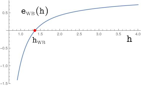
The function $\mathtt{e}_{\scriptscriptstyle{\textsc{WB}}}(\mathtt{h})$ is well defined for any $\mathtt{h}>0$ because the denominator $\mathtt{h}-\tfrac{1}{4}\mathtt{e}_{12}^{2}>0$ in (1.1) is positive for any $\mathtt{h}>0$ , see Lemma 5.7. The function (1.1) coincides, up to a non zero factor, with the celebrated function obtained by Whitham [41], Benjamin [2] and Bridges-Mielke [9] which determines the “shallow/sufficiently deep” threshold regime. In particular the Whitham-Benjamin function $\mathtt{e}_{\scriptscriptstyle{\textsc{WB}}}(\mathtt{h})$ vanishes at $\mathtt{h}_{\scriptscriptstyle{\textsc{WB}}}=1.363...$ , it is negative for $0<\mathtt{h}<\mathtt{h}_{\scriptscriptstyle{\textsc{WB}}}$ , positive for $\mathtt{h}>\mathtt{h}_{\scriptscriptstyle{\textsc{WB}}}$ and tends to $1$ as $\mathtt{h}\to+\infty$ , see Figure 1. We also introduce the positive coefficient

\mathtt{e}_{22}:=\mathtt{e}_{22}(\mathtt{h}):=\dfrac{(1-{\mathtt{c}}_{\mathtt{h}}^{4})(1+3{\mathtt{c}}_{\mathtt{h}}^{4})\mathtt{h}^{2}+2{\mathtt{c}}_{\mathtt{h}}^{2}({\mathtt{c}}_{\mathtt{h}}^{4}-1)\mathtt{h}+{\mathtt{c}}_{\mathtt{h}}^{4}}{{\mathtt{c}}_{\mathtt{h}}^{3}}>0\,,\quad\forall\mathtt{h}>0\,.

(1.3)

We remark that the functions $\mathtt{e}_{12}(\mathtt{h})>{\mathtt{c}}_{\mathtt{h}}$ and $\mathtt{e}_{22}(\mathtt{h})>0$ are positive for any $\mathtt{h}>0$ , tend to $0$ as $\mathtt{h}\to 0^{+}$ and to $1$ as $\mathtt{h}\to+\infty$ , see Lemma 4.8.

Refer to caption — Figure 1: Plot of the Whitham-Benjamin function $\mathtt{e}_{\scriptscriptstyle{\textsc{WB}}}(\mathtt{h})$ . The red dot shows its unique root $\mathtt{h}_{\scriptscriptstyle{\textsc{WB}}}=1.363\dots$ . which is the celebrated “shallow/sufficiently deep” water threshold predicted independently by Whitham (cfr.[41] p.49) and Benjamin (cfr.[2] p.68), and recovered in the rigorous proof of Bridges-Mielke [9, p. 183].

Along the paper we denote by $r(\epsilon^{m_{1}}\mu^{n_{1}},\ldots,\epsilon^{m_{p}}\mu^{n_{p}})$ a real analytic function fulfilling for some $C>0$ and $\epsilon,\mu$ sufficiently small, the estimate $|r(\epsilon^{m_{1}}\mu^{n_{1}},\ldots,\epsilon^{m_{p}}\mu^{n_{p}})|\leq C\sum_{j=1}^{p}|\epsilon|^{m_{j}}|\mu|^{n_{j}}$ , where the constant $C:=C(\mathtt{h})$ is uniform for $\mathtt{h}$ in any compact set of $(0,+\infty)$ .

Theorem 1.1.

(Benjamin-Feir unstable eigenvalues) For any $\mathtt{h}>\mathtt{h}_{\scriptscriptstyle{\textsc{WB}}}$ , there exist $\epsilon_{1},\mu_{0}>0$ and an analytic function $\underline{\mu}:[0,\epsilon_{1})\to[0,\mu_{0})$ , of the form

\underline{\mu}(\epsilon)=\mathtt{e}_{\mathtt{h}}\epsilon(1+r(\epsilon))\,,\quad\mathtt{e}_{\mathtt{h}}:=\sqrt{\frac{8\mathtt{e}_{\scriptscriptstyle{\textsc{WB}}}(\mathtt{h})}{\mathtt{e}_{22}(\mathtt{h})}}\,,

(1.4)

such that, for any $\epsilon\in[0,\epsilon_{1})$ , the operator $\mathcal{L}_{\mu,\epsilon}$ has two eigenvalues $\lambda^{\pm}_{1}(\mu,\epsilon)$ of the form

\begin{cases}\mathrm{i}\,\frac{1}{2}\breve{\mathtt{c}}_{\mathtt{h}}\mu+\mathrm{i}\,r_{2}(\mu\epsilon^{2},\mu^{2}\epsilon,\mu^{3})\pm\tfrac{1}{8}\mu\sqrt{\mathtt{e}_{22}(\mathtt{h})}(1+r(\epsilon,\mu))\sqrt{\Delta_{\scriptscriptstyle{\textsc{BF}}}(\mathtt{h};\mu,\epsilon)},&\forall\mu\in[0,\underline{\mu}(\epsilon))\\[4.2679pt] \mathrm{i}\,\frac{1}{2}\breve{\mathtt{c}}_{\mathtt{h}}\underline{\mu}(\epsilon)+\mathrm{i}\,r(\epsilon^{3}),&\mu=\underline{\mu}(\epsilon)\\[4.2679pt] \mathrm{i}\,\frac{1}{2}\breve{\mathtt{c}}_{\mathtt{h}}\mu+\mathrm{i}\,r_{2}(\mu\epsilon^{2},\mu^{2}\epsilon,\mu^{3})\pm\mathrm{i}\,\tfrac{1}{8}\mu\sqrt{\mathtt{e}_{22}(\mathtt{h})}(1+r(\epsilon,\mu))\sqrt{|\Delta_{\scriptscriptstyle{\textsc{BF}}}(\mathtt{h};\mu,\epsilon)|},&\forall\mu\in(\underline{\mu}(\epsilon),\mu_{0})\end{cases}\!\!\!

(1.5)

where $\breve{\mathtt{c}}_{\mathtt{h}}:=2{\mathtt{c}}_{\mathtt{h}}-\mathtt{e}_{12}(\mathtt{h})>0$ and $\Delta_{\scriptscriptstyle{\textsc{BF}}}(\mathtt{h};\mu,\epsilon)$ is the “Benjamin-Feir discriminant” function

\Delta_{\scriptscriptstyle{\textsc{BF}}}(\mathtt{h};\mu,\epsilon):=8\mathtt{e}_{\scriptscriptstyle{\textsc{WB}}}(\mathtt{h})\epsilon^{2}+r_{1}(\epsilon^{3},\mu\epsilon^{2})-\mathtt{e}_{22}(\mathtt{h})\mu^{2}\big(1+r_{1}^{\prime\prime}(\epsilon,\mu)\big)\,.

(1.6)

Note that, for any $0<\epsilon<\epsilon_{1}$ (depending on $\mathtt{h}$ ) the function $\Delta_{\scriptscriptstyle{\textsc{BF}}}(\mathtt{h};\mu,\epsilon)>0$ is positive, respectively $<0$ , provided $0<\mu<\underline{\mu}(\epsilon)$ , respectively $\mu>\underline{\mu}(\epsilon)$ .

Let us make some comments.
1. Benjamin-Feir unstable eigenvalues. For $\mathtt{h}>\mathtt{h}_{\scriptscriptstyle{\textsc{WB}}}$ , according to (1.5), for values of the Floquet parameter $0<\mu<\underline{\mu}(\epsilon)$ , the eigenvalues $\lambda^{\pm}_{1}(\mu,\epsilon)$ have opposite non-zero real part. As $\mu$ tends to $\underline{\mu}(\epsilon)$ , the two eigenvalues $\lambda^{\pm}_{1}(\mu,\epsilon)$ collide on the imaginary axis far from $0$ (in the upper semiplane $\text{Im}(\lambda)>0$ ), along which they keep moving for $\mu>\underline{\mu}(\epsilon)$ , see Figure 2. For $\mu<0$ the operator ${\mathcal{L}}_{\mu,\epsilon}$ possesses the symmetric eigenvalues $\overline{\lambda_{1}^{\pm}(-\mu,\epsilon)}$ in the semiplane $\text{Im}(\lambda)<0$ . For $\mu\in[0,\underline{\mu}(\epsilon)]$ we obtain the upper part of the figure “8”, which is well approximated by the curves

\mu\mapsto\Big(\pm\frac{\mu}{8}\sqrt{\mathtt{e}_{22}}\sqrt{8\mathtt{e}_{\scriptscriptstyle{\textsc{WB}}}\epsilon^{2}-\mathtt{e}_{22}\mu^{2}},\ \tfrac{1}{2}\breve{\mathtt{c}}_{\mathtt{h}}\mu\Big)\,,

(1.7)

in accordance with the numerical simulations by Deconinck-Oliveras [15]. Note that for $\mu>0$ the imaginary part in (1.7) is positive because $\breve{\mathtt{c}}_{\mathtt{h}}={\mathtt{c}}_{\mathtt{h}}^{-1}(\tanh(\mathtt{h})-(1-\tanh^{2}(\mathtt{h}))\mathtt{h})>0$ for any $\mathtt{h}>0$ . The higher order “side-band” corrections of the eigenvalues $\lambda_{1}^{\pm}(\mu,\epsilon)$ in (1.5), provided by the analytic functions $r,r_{1},r_{1}^{\prime\prime},r_{2}$ , are explicitly computable. We finally remark that the eigenvalues (1.5) are not analytic in $(\mu,\epsilon)$ close to the value $(\underline{\mu}(\epsilon),\epsilon)$ where $\lambda^{\pm}_{1}(\mu,\epsilon)$ collide at the top of the figure $``8"$ far from $0$ (clearly they are continuous).

2. Behaviour near the Whitham-Benjamin depth $\mathtt{h}_{\scriptscriptstyle{\textsc{WB}}}$ . As ${\mathtt{h}}\to\mathtt{h}_{\scriptscriptstyle{\textsc{WB}}}^{+}$ the constant $\epsilon_{1}:=\epsilon_{1}(\mathtt{h})>0$ in Theorem 1.1 tends to zero, the set of unstable Floquet exponents $(0,\underline{\mu}(\epsilon))$ with $\underline{\mu}(\epsilon)=\mathtt{e}_{\mathtt{h}}\epsilon(1+r(\epsilon))$ given in (1.4) shrinks to zero and the figure “8” of Benjamin-Feir unstable eigenvalues collapse to zero, see Figure 3. In particular

\max_{\mu\in[0,\underline{\mu}(\epsilon)]}\text{Re}\,\lambda_{1}^{+}(\mu,\epsilon)=\text{Re}\,\lambda_{1}^{+}(\mu_{\max},\epsilon)=\frac{1}{2}{\mathtt{e}_{\scriptscriptstyle{\textsc{WB}}}}(\mathtt{h})\epsilon^{2}+r(\epsilon^{3})\ \text{ and }

(1.8)

tends to zero as $\mathtt{h}\to\mathtt{h}_{\scriptscriptstyle{\textsc{WB}}}^{+}$ , since $0<\epsilon<\epsilon_{1}(\mathtt{h})$ and $\epsilon_{1}(\mathtt{h})\to 0^{+}$ .

3. Relation with Bridges-Mielke [9]. Bridges and Mielke describe the unstable eigenvalues very close to the origin, namely the cross amid the ‘8”. In order to make a precise comparison with our result let us spell out the relation of the functions $\mathtt{e}_{\scriptscriptstyle{\textsc{WB}}}$ , $\mathtt{e}_{12}$ and $\mathtt{e}_{22}$ with the coefficients obtained in [9]. The Whitham-Benjamin function $\mathtt{e}_{\scriptscriptstyle{\textsc{WB}}}$ in (4.13) is $\mathtt{e}_{\scriptscriptstyle{\textsc{WB}}}=({\mathtt{c}}_{\mathtt{h}}\mathtt{h})^{-1}\nu(F)$ , where $\nu(F)$ is defined in [9, formula (6.17)] and $F={\mathtt{c}}_{\mathtt{h}}\mathtt{h}^{-\frac{1}{2}}$ is the Froude number, cfr. [9, formula (3.4)]. Moreover the term $\mathtt{e}_{12}$ in (1.2) is $\mathtt{e}_{12}=2c_{g}$ , where $c_{g}=\frac{1}{2}{\mathtt{c}}_{\mathtt{h}}\big(1+F^{-2}\text{sech}^{2}(\mathtt{h})\big)$ is the group velocity defined in Bridges-Mielke [9, formula (3.8)]. Finally $\mathtt{e}_{22}(\mathtt{h})\propto\dot{c}_{g}$ where $\dot{c}_{g}$ is the derivative of the group velocity defined in [9, formula (6.15)], which for gravity waves is negative in any depth.
4. Complete spectrum near $0$ . In Theorem 1.1 we have described just the two unstable eigenvalues of $\mathcal{L}_{\mu,\epsilon}$ close to zero for $\mathtt{h}>\mathtt{h}_{\scriptscriptstyle{\textsc{WB}}}$ . There are also two larger purely imaginary eigenvalues of order $\mathcal{O}(\mu)$ , see Theorem 2.5. We remark that our approach describes all the eigenvalues of ${\mathcal{L}}_{\mu,\epsilon}$ close to $0$ (which are $4$ ).
5. Shallow water regime. In the shallow water regime $0<\mathtt{h}<\mathtt{h}_{\scriptscriptstyle{\textsc{WB}}}$ , we prove in Theorem 2.5 that all the four eigenvalues of ${\mathcal{L}}_{\mu,\epsilon}$ close to zero remain purely imaginary for $\epsilon$ sufficiently small. The eigenvalue expansions of Theorem 2.5 become singular as $\mathtt{h}\to 0^{+}$ .
6. Behavior at the Whitham-Benjamin threshold $\mathtt{h}_{\scriptscriptstyle{\textsc{WB}}}$ . The analysis of Theorem 1.1 is not conclusive at the critical depth $\mathtt{h}=\mathtt{h}_{\scriptscriptstyle{\textsc{WB}}}$ . The reason is that $\mathtt{e}_{\scriptscriptstyle{\textsc{WB}}}(\mathtt{h}_{\scriptscriptstyle{\textsc{WB}}})=0$ and the Benjamin-Feir discriminant function (1.6) reduces to

\Delta_{\scriptscriptstyle{\textsc{BF}}}(\mathtt{h}_{\scriptscriptstyle{\textsc{WB}}};\mu,\epsilon)=r(\epsilon^{3})+r(\mu\epsilon^{2})-\mathtt{e}_{22}(\mathtt{h}_{\scriptscriptstyle{\textsc{WB}}})\mu^{2}(1+r_{1}^{\prime\prime}(\epsilon,\mu))\,.

(1.9)

Thus its quadratic expansion is not sufficient anymore to determine the sign of $\Delta_{\scriptscriptstyle{\textsc{BF}}}(\mathtt{h}_{\scriptscriptstyle{\textsc{WB}}};\mu,\epsilon)$ . Note that (1.9) could be positive due to the cubic term $r(\epsilon^{3})=\alpha\epsilon^{3}+\dots$ for $\epsilon$ and $\mu$ small enough. The coefficient $\alpha$ could be explicitly computed taking into account the third order expansion of the Stokes waves.
7. Unstable Floquet exponents and amplitudes $(\mu,\epsilon)$ . In Theorem 2.5 we actually prove that the expansion (1.5) of the eigenvalues of $\mathcal{L}_{\mu,\epsilon}$ holds for any value of $(\mu,\epsilon)$ in a larger rectangle $[0,\mu_{0})\times[0,\epsilon_{0})$ , and there exist Benjamin-Feir unstable eigenvalues if and only if the analytic function $\Delta_{\scriptscriptstyle{\textsc{BF}}}(\mathtt{h};\mu,\epsilon)$ in (1.6) is positive. The zero set of $\Delta_{\scriptscriptstyle{\textsc{BF}}}(\mathtt{h};\mu,\epsilon)$ is an analytic variety which, for $\mathtt{h}>\mathtt{h}_{\scriptscriptstyle{\textsc{WB}}}$ , is, restricted to the rectangle $[0,\mu_{0})\times[0,\epsilon_{1})$ , the graph of the analytic function $\underline{\mu}(\epsilon)=\mathtt{e}_{\mathtt{h}}\epsilon(1+r(\epsilon))$ in (1.4). This function is tangent at $\epsilon=0$ to the straight line $\mu=\mathtt{e}_{\mathtt{h}}\epsilon$ , and divides $[0,\mu_{0})\times[0,\epsilon_{1})$ in the region where $\Delta_{\scriptscriptstyle{\textsc{BF}}}(\mathtt{h};\mu,\epsilon)>0$ –and thus the eigenvalues of ${\mathcal{L}}_{\mu,\epsilon}$ have non-trivial real part–, from the “stable” one where all the eigenvalues of ${\mathcal{L}}_{\mu,\epsilon}$ are purely imaginary, see Figure 4. In the region $[0,\mu_{0})\times[\epsilon_{1},\epsilon_{0})$ the higher order polynomial approximations of $\Delta_{\scriptscriptstyle{\textsc{BF}}}(\mathtt{h};\mu,\epsilon)$ (which are computable) will determine the sign of $\Delta_{\scriptscriptstyle{\textsc{BF}}}(\mathtt{h};\mu,\epsilon)$ .

8. Deep water limit. Theorems 1.1 and 2.5 do not pass to the limit as $\mathtt{h}\to+\infty$ since the remainders in the expansions of the eigenvalues are uniform only on any compact set of $\mathtt{h}\in(0,+\infty)$ . From a mathematical point of view, the difference is evident in the asymptotic behavior of $\tanh(\mathtt{h}\mu)$ (and similar quantities) which, in the idealized deep water case $\mathtt{h}=+\infty$ , is identically equal to $1$ for any arbitrarily small Floquet exponent $\mu$ , whereas $\tanh(\mathtt{h}\mu)=O(\mu\mathtt{h})$ for any $\mathtt{h}$ finite. However additional intermediate scaling regimes $\mathtt{h}\mu\sim 1$ , $\mathtt{h}\mu\ll 1$ , $\mathtt{h}\mu\gg 1$ are possible. It is well-known (e.g. see [14]) that intermediate long-wave regimes of the water-waves equations formally lead to different physically-relevant limit equations as Boussinesq, KdV, NLS, Benjamin-Ono, etc…

We shall describe in detail the ideas of proof and the differences with the deep water case below the statement of Theorem 2.5.
Further literature. Modulational instability has been studied also for a variety of approximate water waves models, such as KdV, gKdV, NLS and the Whitham equation by, for instance, Whitham [42], Segur, Henderson, Carter and Hammack [37], Gallay and Haragus [17], Haragus and Kapitula [19], Bronski and Johnson [11], Johnson [25], Hur and Johnson [21], Bronski, Hur and Johnson [10], Hur and Pandey [22], Leisman, Bronski, Johnson and Marangell [30]. Also for these approximate models, numerical simulations predict a figure “8” similar to that in Figure 2 for the bifurcation of the unstable eigenvalues close to zero. We expect the present approach can be adapted to describe the full bifurcation of the eigenvalues also for these models.

Finally we mention the nonlinear modulational instability result of Jin, Liao, and Lin [24] for several fluid model equations and the preprint by Chen-Su [12] for Stokes waves in deep water. Nonlinear transversal instability results of traveling solitary water waves in finite depth decaying at infinity on $\mathbb{R}$ have been proved in [36] (in deep water no solitary wave exists [20, 27]).
Acknowledgments. Research supported by PRIN 2020 (2020XB3EFL001) “Hamiltonian and dispersive PDEs”.

2 The complete Benjamin-Feir spectrum in finite depth

In this section we present in detail the complete spectral Theorem 2.5. We first introduce the pure gravity water waves equations and the Stokes waves solutions.
The water waves equations. We consider the Euler equations for a 2-dimensional incompressible, irrotational fluid under the action of gravity. The fluid fills the region

{\mathcal{D}}_{\eta}:=\left\{(x,y)\in\mathbb{T}\times\mathbb{R}\;:\;-\mathtt{h}\leq y<\eta(t,x)\right\}\,,\quad\mathbb{T}:=\mathbb{R}/2\pi\mathbb{Z}\,,

with finite depth and space periodic boundary conditions. The irrotational velocity field is the gradient of a harmonic scalar potential $\Phi=\Phi(t,x,y)$ determined by its trace $\psi(t,x)=\Phi(t,x,\eta(t,x))$ at the free surface $y=\eta(t,x)$ . Actually $\Phi$ is the unique solution of the elliptic equation $\Delta\Phi=0$ in ${\mathcal{D}}_{\eta}$ with Dirichlet datum $\Phi(t,x,\eta(t,x))=\psi(t,x)$ and $\Phi_{y}(t,x,y)=0$ at $y=-\mathtt{h}$ .

The time evolution of the fluid is determined by two boundary conditions at the free surface. The first is that the fluid particles remain, along the evolution, on the free surface (kinematic boundary condition), and the second one is that the pressure of the fluid is equal, at the free surface, to the constant atmospheric pressure (dynamic boundary condition). Then, as shown by Zakharov [44] and Craig-Sulem [13], the time evolution of the fluid is determined by the following equations for the unknowns $(\eta(t,x),\psi(t,x))$ ,

\eta_{t}=G(\eta)\psi\,,\quad\psi_{t}=-g\eta-\dfrac{\psi_{x}^{2}}{2}+\dfrac{1}{2(1+\eta_{x}^{2})}\big(G(\eta)\psi+\eta_{x}\psi_{x}\big)^{2}\,,

(2.1)

where $g>0$ is the gravity constant and $G(\eta):=G(\eta,\mathtt{h})$ denotes the Dirichlet-Neumann operator $[G(\eta)\psi](x):=\Phi_{y}(x,\eta(x))-\Phi_{x}(x,\eta(x))\eta_{x}(x)$ . In the sequel, with no loss of generality, we set the gravity constant $g=1$ , see Remark 2.4.

The equations (2.1) are the Hamiltonian system

\partial_{t}\begin{bmatrix}\eta\\ \psi\end{bmatrix}=\mathcal{J}\begin{bmatrix}\nabla_{\eta}\mathcal{H}\\ \nabla_{\psi}\mathcal{H}\end{bmatrix},\quad\quad\mathcal{J}:=\begin{bmatrix}0&\mathrm{Id}\\ -\mathrm{Id}&0\end{bmatrix},

(2.2)

where $\nabla$ denote the $L^{2}$ -gradient, and the Hamiltonian $\mathcal{H}(\eta,\psi):=\frac{1}{2}\int_{\mathbb{T}}\left(\psi\,G(\eta)\psi+\eta^{2}\right)\mathrm{d}x$ is the sum of the kinetic and potential energy of the fluid. In addition of being Hamiltonian, the water waves system (2.1) possesses other important symmetries. First of all it is time reversible with respect to the involution

\rho\begin{bmatrix}\eta(x)\\ \psi(x)\end{bmatrix}:=\begin{bmatrix}\eta(-x)\\ -\psi(-x)\end{bmatrix},\quad\text{i.e. }\mathcal{H}\circ\rho=\mathcal{H}\,.

(2.3)

Moreover, the equation (2.1) is space invariant, since, being the bottom flat,

\tau_{\theta}G(\eta)\psi=G(\tau_{\theta}\eta)[\tau_{\theta}\psi]\,,\quad\forall\theta\in\mathbb{R}\,,\quad\text{where}\quad\tau_{\theta}u(x):=u(x+\theta)\,.

In addition, the Dirichlet-Neumann operator satisfies $G(\eta+m,\mathtt{h})=G(\eta,\mathtt{h}+m)$ , for any $m\in\mathbb{R}$ .
Stokes waves. The Stokes waves are traveling solutions of (2.1) of the form $\eta(t,x)=\breve{\eta}(x-ct)$ and $\psi(t,x)=\breve{\psi}(x-ct)$ for some real $c$ and $2\pi$ -periodic functions $(\breve{\eta}(x),\breve{\psi}(x))$ . In a reference frame in translational motion with constant speed $c$ , the water waves equations (2.1) become

\eta_{t}=c\eta_{x}+G(\eta)\psi\,,\quad\psi_{t}=c\psi_{x}-\eta-\dfrac{\psi_{x}^{2}}{2}+\dfrac{1}{2(1+\eta_{x}^{2})}\big(G(\eta)\psi+\eta_{x}\psi_{x}\big)^{2}

(2.4)

and the Stokes waves $(\breve{\eta},\breve{\psi})$ are equilibrium steady solutions of (2.4).

The bifurcation result of small amplitude of Stokes waves is due to Struik [39] in finite depth, and Levi-Civita [31], and Nekrasov [34] in infinite depth. We denote by $B(r):=\{x\in\mathbb{R}\colon\ |x|<r\}$ the real ball with center 0 and radius $r$ .

Theorem 2.1.

(Stokes waves) For any $\mathtt{h}>0$ there exist $\epsilon_{*}:=\epsilon_{*}(\mathtt{h})>0$ and a unique family of real analytic solutions $(\eta_{\epsilon}(x),\psi_{\epsilon}(x),c_{\epsilon})$ , parameterized by the amplitude $|\epsilon|\leq\epsilon_{*}$ , of

c\,\eta_{x}+G(\eta)\psi=0\,,\quad c\,\psi_{x}-\eta-\dfrac{\psi_{x}^{2}}{2}+\dfrac{1}{2(1+\eta_{x}^{2})}\big(G(\eta)\psi+\eta_{x}\psi_{x}\big)^{2}=0\,,

(2.5)

such that $\eta_{\epsilon}(x),\psi_{\epsilon}(x)$ are $2\pi$ -periodic; $\eta_{\epsilon}(x)$ is even and $\psi_{\epsilon}(x)$ is odd, of the form

		$\displaystyle\eta_{\epsilon}(x)=\epsilon\cos(x)+\epsilon^{2}(\eta_{2}^{[0]}+\eta_{2}^{[2]}\cos(2x))+\mathcal{O}(\epsilon^{3}),$		(2.6)
		$\displaystyle\psi_{\epsilon}(x)=\epsilon{\mathtt{c}}_{\mathtt{h}}^{-1}\sin(x)+\epsilon^{2}\psi_{2}^{[2]}\sin(2x)+\mathcal{O}(\epsilon^{3})\,,$
		$\displaystyle c_{\epsilon}={\mathtt{c}}_{\mathtt{h}}+\epsilon^{2}c_{2}+\mathcal{O}(\epsilon^{3})\quad\text{where}\quad{\mathtt{c}}_{\mathtt{h}}=\sqrt{\tanh(\mathtt{h})}\,,$

and

	$\displaystyle\eta_{2}^{[0]}:=\frac{{\mathtt{c}}_{\mathtt{h}}^{4}-1}{4{\mathtt{c}}_{\mathtt{h}}^{2}}\,,\qquad\eta_{2}^{[2]}:=\frac{3-{\mathtt{c}}_{\mathtt{h}}^{4}}{4{\mathtt{c}}_{\mathtt{h}}^{6}}\,,\qquad\psi_{2}^{[2]}:=\frac{3+{\mathtt{c}}_{\mathtt{h}}^{8}}{8{\mathtt{c}}_{\mathtt{h}}^{7}}\,,\qquad$		(2.7)
	$\displaystyle c_{2}:=\frac{9-10{\mathtt{c}}_{\mathtt{h}}^{4}+9{\mathtt{c}}_{\mathtt{h}}^{8}}{16{\mathtt{c}}_{\mathtt{h}}^{7}}+{\frac{(1-{\mathtt{c}}_{\mathtt{h}}^{4})}{2{\mathtt{c}}_{\mathtt{h}}}}\eta_{2}^{[0]}=\frac{-2{\mathtt{c}}_{\mathtt{h}}^{12}+13{\mathtt{c}}_{\mathtt{h}}^{8}-12{\mathtt{c}}_{\mathtt{h}}^{4}+9}{16{\mathtt{c}}_{\mathtt{h}}^{7}}\,.$		(2.8)

More precisely for any $\sigma\geq 0$ and $s>\frac{5}{2}$ , there exists $\epsilon_{*}>0$ such that the map $\epsilon\mapsto(\eta_{\epsilon},\psi_{\epsilon},c_{\epsilon})$ is analytic from $B(\epsilon_{*})\to H^{\sigma,s}_{\mathtt{ev}}(\mathbb{T})\times H^{\sigma,s}_{\mathtt{odd}}(\mathbb{T})\times\mathbb{R}$ , where $H^{\sigma,s}_{\mathtt{ev}}(\mathbb{T})$ , respectively $H^{\sigma,s}_{\mathtt{odd}}(\mathbb{T})$ , denote the space of even, respectively odd, real valued $2\pi$ -periodic analytic functions $u(x)=\sum_{k\in\mathbb{Z}}u_{k}e^{\mathrm{i}\,kx}$ such that $\|u\|_{\sigma,s}^{2}:=\sum_{k\in\mathbb{Z}}|u_{k}|^{2}\langle k\rangle^{2s}e^{2\sigma|k|}<+\infty$ .

The expansions (2.6)-(2.8) are derived in the Appendix B for completeness, although present in the literature (they coincide with [42, section 13, chapter 13] and [2, section 2]). Note that in the shallow water regime $\mathtt{h}\to 0^{+}$ the expansions (2.6)-(2.8) become singular. For the analiticity properties of the maps stated in Theorem 2.1 we refer to [8].

We also mention that more general time quasi-periodic traveling Stokes waves – which are nonlinear superpositions of multiple Stokes waves traveling with rationally independent speeds – have been recently proved for (2.1) in [5] in finite depth, in [16] in infinite depth, and in [4] for capillary-gravity water waves in any depth.
Linearization at the Stokes waves. In order to determine the stability/instability of the Stokes waves given by Theorem 2.1, we linearize the water waves equations (2.4) with $c=c_{\epsilon}$ at $(\eta_{\epsilon}(x),\psi_{\epsilon}(x))$ . In the sequel we closely follow [6] pointing out the differences of the finite depth case.

By using the shape derivative formula for the differential $\mathrm{d}_{\eta}G(\eta)[\hat{\eta}]$ of the Dirichlet-Neumann operator one obtains the autonomous real linear system

\begin{bmatrix}\hat{\eta}_{t}\\ \hat{\psi}_{t}\end{bmatrix}=\begin{bmatrix}-G(\eta_{\epsilon})B-\partial_{x}\circ(V-c_{\epsilon})&G(\eta_{\epsilon})\\ -1+B(V-c_{\epsilon})\partial_{x}-B\partial_{x}\circ(V-c_{\epsilon})-BG(\eta_{\epsilon})\circ B&-(V-c_{\epsilon})\partial_{x}+BG(\eta_{\epsilon})\end{bmatrix}\begin{bmatrix}\hat{\eta}\\ \hat{\psi}\end{bmatrix}

(2.9)

where

V:=V(x):=-B(\eta_{\epsilon})_{x}+(\psi_{\epsilon})_{x}\,,\ \ B:=B(x):=\frac{G(\eta_{\epsilon})\psi_{\epsilon}+(\psi_{\epsilon})_{x}(\eta_{\epsilon})_{x}}{1+(\eta_{\epsilon})_{x}^{2}}=\frac{(\psi_{\epsilon})_{x}-c_{\epsilon}}{1+(\eta_{\epsilon})_{x}^{2}}(\eta_{\epsilon})_{x}\,.

(2.10)

The functions $(V,B)$ are the horizontal and vertical components of the velocity field $(\Phi_{x},\Phi_{y})$ at the free surface. Moreover $\epsilon\mapsto(V,B)$ is analytic as a map $B(\epsilon_{0})\to H^{\sigma,s-1}(\mathbb{T})\times H^{\sigma,s-1}(\mathbb{T})$ .

The real system (2.9) is Hamiltonian, i.e. of the form $\mathcal{J}\mathcal{A}$ for a symmetric operator $\mathcal{A}=\mathcal{A}^{\top}$ , where $\mathcal{A}^{\top}$ is the transposed operator with respect the standard real scalar product of $L^{2}(\mathbb{T},\mathbb{R})\times L^{2}(\mathbb{T},\mathbb{R})$ .

Moreover, since $\eta_{\epsilon}$ is even in $x$ and $\psi_{\epsilon}$ is odd in $x$ , then the functions $(V,B)$ are respectively even and odd in $x$ , and the linear operator in (2.9) is reversible, i.e. it anti-commutes with the involution $\rho$ in (2.3).

Under the time-independent “good unknown of Alinhac” linear transformation

\begin{bmatrix}\hat{\eta}\\ \hat{\psi}\end{bmatrix}:=Z\begin{bmatrix}u\\ v\end{bmatrix}\,,\qquad Z=\begin{bmatrix}1&0\\ B&1\end{bmatrix},\quad Z^{-1}=\begin{bmatrix}1&0\\ -B&1\end{bmatrix},

(2.11)

the system (2.9) assumes the simpler form

\begin{bmatrix}u_{t}\\ v_{t}\end{bmatrix}=\widetilde{\mathcal{L}}_{\epsilon}\begin{bmatrix}u\\ v\end{bmatrix},\qquad\widetilde{\mathcal{L}}_{\epsilon}:=\begin{bmatrix}-\partial_{x}\circ(V-c_{\epsilon})&G(\eta_{\epsilon})\\ -1-(V-c_{\epsilon})B_{x}&-(V-c_{\epsilon})\partial_{x}\end{bmatrix}\,.

(2.12)

Note that, since the transformation $Z$ is symplectic, i.e. $Z^{\top}\mathcal{J}Z=\mathcal{J}$ , and reversibility preserving, i.e. $Z\circ\rho=\rho\circ Z$ , the linear system (2.12) is Hamiltonian and reversible as (2.9).

Next we perform a conformal change of variables to flatten the water surface. Here the finite depth case induces a modification with respect to the deep water case. By [1, Appendix A], there exists a diffeomorphism of $\mathbb{T}$ , $x\mapsto x+\mathfrak{p}(x)$ , with a small $2\pi$ -periodic function $\mathfrak{p}(x)$ , and a small constant $\mathtt{f}_{\epsilon}$ , such that, by defining the associated composition operator $(\mathfrak{P}u)(x):=u(x+\mathfrak{p}(x))$ , the Dirichlet-Neumann operator writes as [1, Lemma A.5]

G(\eta_{\epsilon})=\partial_{x}\circ\mathfrak{P}^{-1}\circ{\mathcal{H}}\circ\tanh\big((\mathtt{h}+\mathtt{f}_{\epsilon})|D|\big)\circ\mathfrak{P}\,,

(2.13)

where ${\mathcal{H}}$ is the Hilbert transform, i.e. the Fourier multiplier operator

\mathcal{H}(e^{\mathrm{i}\,jx}):=-\mathrm{i}\,\textup{sign}(j)e^{\mathrm{i}\,jx}\,,\quad\forall j\in\mathbb{Z}\setminus\{0\}\,,\quad\mathcal{H}(1):=0\,.

The function $\mathfrak{p}(x)$ and the constant $\mathtt{f}_{\epsilon}$ are determined as a fixed point of (see [1, formula (A.15)])

\mathfrak{p}=\frac{\mathcal{H}}{\tanh\big((\mathtt{h}+\mathtt{f}_{\epsilon})|D|\big)}[\eta_{\epsilon}(x+\mathfrak{p}(x))]\,,\qquad\mathtt{f}_{\epsilon}:=\frac{1}{2\pi}\int_{\mathbb{T}}\eta_{\epsilon}(x+\mathfrak{p}(x))\mathrm{d}x\,.

(2.14)

By the analyticity of the map $\epsilon\to\eta_{\epsilon}\in H^{\sigma,s}$ , $\sigma>0$ , $s>1/2$ , the analytic implicit function theorem implies the existence of a solution $\epsilon\mapsto\mathfrak{p}(x):=\mathfrak{p}_{\epsilon}(x)$ , $\epsilon\mapsto\mathtt{f}_{\epsilon}$ , analytic as a map $B(\epsilon_{0})\to H^{s}(\mathbb{T})\times\mathbb{R}$ . Moreover, since $\eta_{\epsilon}$ is even, the function $\mathfrak{p}(x)$ is odd. In Appendix B we prove the expansion

\mathfrak{p}(x)=\epsilon{\mathtt{c}}_{\mathtt{h}}^{-2}\sin(x)+\epsilon^{2}\frac{(1+{\mathtt{c}}_{\mathtt{h}}^{4})(3+{\mathtt{c}}_{\mathtt{h}}^{4})}{8{\mathtt{c}}_{\mathtt{h}}^{8}}\sin(2x)+\mathcal{O}(\epsilon^{3})\,,\quad\mathtt{f}_{\epsilon}=\epsilon^{2}\frac{{\mathtt{c}}_{\mathtt{h}}^{4}-3}{4{\mathtt{c}}_{\mathtt{h}}^{2}}+\mathcal{O}(\epsilon^{3})\,.

(2.15)

Under the symplectic and reversibility-preserving map

\mathcal{P}:=\begin{bmatrix}(1+\mathfrak{p}_{x})\mathfrak{P}&0\\ 0&\mathfrak{P}\end{bmatrix}\,,

(2.16)

the system (2.12) transforms, by (2.13), into the linear system $h_{t}=\mathcal{L}_{\epsilon}h$ where $\mathcal{L}_{\epsilon}$ is the Hamiltonian and reversible real operator

	$\displaystyle\mathcal{L}_{\epsilon}:=\mathcal{P}\,\widetilde{\mathcal{L}}_{\epsilon}\,\mathcal{P}^{-1}$	$\displaystyle=\begin{bmatrix}\partial_{x}\circ({\mathtt{c}}_{\mathtt{h}}+p_{\epsilon}(x))&\|D\|\tanh((\mathtt{h}+\mathtt{f}_{\epsilon})\|D\|)\\ -(1+a_{\epsilon}(x))&({\mathtt{c}}_{\mathtt{h}}+p_{\epsilon}(x))\partial_{x}\end{bmatrix}$		(2.17)
		$\displaystyle=\mathcal{J}\begin{bmatrix}1+a_{\epsilon}(x)&-({\mathtt{c}}_{\mathtt{h}}+p_{\epsilon}(x))\partial_{x}\\ \partial_{x}\circ({\mathtt{c}}_{\mathtt{h}}+p_{\epsilon}(x))&\|D\|\tanh((\mathtt{h}+\mathtt{f}_{\epsilon})\|D\|)\end{bmatrix}$		(2.17)

where

{\mathtt{c}}_{\mathtt{h}}+p_{\epsilon}(x):=\displaystyle{\frac{c_{\epsilon}-V(x+\mathfrak{p}(x))}{1+\mathfrak{p}_{x}(x)}}\,,\quad 1+a_{\epsilon}(x):=\displaystyle{\frac{1+(V(x+\mathfrak{p}(x))-c_{\epsilon})B_{x}(x+\mathfrak{p}(x))}{1+\mathfrak{p}_{x}(x)}}\,.

(2.18)

By the analiticity results of the functions $V,B,\mathfrak{p}(x)$ given above, the functions $p_{\epsilon}$ and $a_{\epsilon}$ are analytic in $\epsilon$ as maps $B(\epsilon_{0})\to H^{s}(\mathbb{T})$ . In the Appendix B we prove the following expansions.

Lemma 2.2.

The analytic functions $p_{\epsilon}(x)$ and $a_{\epsilon}(x)$ in (2.18) are even in $x$ , and

p_{\epsilon}(x)=\epsilon p_{1}(x)+\epsilon^{2}p_{2}(x)+\mathcal{O}(\epsilon^{3})\,,\qquad a_{\epsilon}(x)=\epsilon a_{1}(x)+\epsilon^{2}a_{2}(x)+\mathcal{O}(\epsilon^{3})\,,

(2.19)

where

	$\displaystyle p_{1}(x)$	$\displaystyle=p_{1}^{[1]}\cos(x)\,,\qquad\quad\quad p_{1}^{[1]}:=-2{\mathtt{c}}_{\mathtt{h}}^{-1}\,,$		(2.20)
	$\displaystyle p_{2}(x)$	$\displaystyle=p_{2}^{[0]}+p_{2}^{[2]}\cos(2x)\,,\quad p_{2}^{[0]}:=\frac{9+12{\mathtt{c}}_{\mathtt{h}}^{4}+5{\mathtt{c}}_{\mathtt{h}}^{8}-2{\mathtt{c}}_{\mathtt{h}}^{12}}{16{\mathtt{c}}_{\mathtt{h}}^{7}}\,,\quad p_{2}^{[2]}:=-\frac{3+{\mathtt{c}}_{\mathtt{h}}^{4}}{2{\mathtt{c}}_{\mathtt{h}}^{7}}\,,$		(2.21)

and

	$\displaystyle a_{1}(x)$	$\displaystyle=a_{1}^{[1]}\cos(x)\,,\qquad\qquad a_{1}^{[1]}:=-({\mathtt{c}}_{\mathtt{h}}^{2}+{\mathtt{c}}_{\mathtt{h}}^{-2})\,,$		(2.22)
	$\displaystyle a_{2}(x)$	$\displaystyle=a_{2}^{[0]}+a_{2}^{[2]}\cos(2x)\,,\quad a_{2}^{[0]}:=\frac{3}{2}+\frac{1}{2{\mathtt{c}}_{\mathtt{h}}^{4}}\,,\quad a_{2}^{[2]}:=\frac{-14{\mathtt{c}}_{\mathtt{h}}^{4}+9{\mathtt{c}}_{\mathtt{h}}^{8}-3}{4{\mathtt{c}}_{\mathtt{h}}^{8}}\,.$		(2.23)

Bloch-Floquet expansion. Since the operator $\mathcal{L}_{\epsilon}$ in (2.17) has $2\pi$ -periodic coefficients, Bloch-Floquet theory guarantees that

\sigma_{L^{2}(\mathbb{R})}(\mathcal{L}_{\epsilon})=\bigcup_{\mu\in[-\frac{1}{2},\frac{1}{2})}\sigma_{L^{2}(\mathbb{T})}(\mathcal{L}_{\mu,\epsilon})\qquad\text{where}\quad\qquad\mathcal{L}_{\mu,\epsilon}:=e^{-\mathrm{i}\,\mu x}\,\mathcal{L}_{\epsilon}\,e^{\mathrm{i}\,\mu x}\,.

The domain $[-\frac{1}{2},\frac{1}{2})$ is called, in solid state physics, the “first zone of Brillouin”. In particular, if $\lambda$ is an eigenvalue of $\mathcal{L}_{\mu,\epsilon}$ on $L^{2}(\mathbb{T},\mathbb{C}^{2})$ with eigenvector $v(x)$ , then $h(t,x)=e^{\lambda t}e^{\mathrm{i}\,\mu x}v(x)$ solves $h_{t}=\mathcal{L}_{\epsilon}h$ . We remark that:
1. If $A=\mathrm{Op}(a)$ is a pseudo-differential operator with symbol $a(x,\xi)$ , which is $2\pi$ periodic in the $x$ -variable, then $A_{\mu}:=e^{-\mathrm{i}\,\mu x}Ae^{\mathrm{i}\,\mu x}=\mathrm{Op}(a(x,\xi+\mu))$ .
2. If $A$ is a real operator then $\overline{A_{\mu}}=A_{-\mu}$ . As a consequence the spectrum $\sigma(A_{-\mu})=\overline{\sigma(A_{\mu})}$ and we can study $\sigma(A_{\mu})$ just for $\mu>0$ . Furthermore $\sigma(A_{\mu})$ is a 1-periodic set with respect to $\mu$ , so one can restrict to $\mu\in[0,\frac{1}{2})$ .

By the previous remarks the Floquet operator associated with the real operator $\mathcal{L}_{\epsilon}$ in (2.17) is the complex Hamiltonian and reversible operator

	$\displaystyle\mathcal{L}_{\mu,\epsilon}:$	$\displaystyle=\begin{bmatrix}(\partial_{x}+\mathrm{i}\,\mu)\circ({\mathtt{c}}_{\mathtt{h}}+p_{\epsilon}(x))&\|D+\mu\|\tanh\big((\mathtt{h}+\mathtt{f}_{\epsilon})\|D+\mu\|\big)\\ -(1+a_{\epsilon}(x))&({\mathtt{c}}_{\mathtt{h}}+p_{\epsilon}(x))(\partial_{x}+\mathrm{i}\,\mu)\end{bmatrix}$		(2.24)
		$\displaystyle=\underbrace{\begin{bmatrix}0&\mathrm{Id}\\ -\mathrm{Id}&0\end{bmatrix}}_{\displaystyle{=\mathcal{J}}}\underbrace{\begin{bmatrix}1+a_{\epsilon}(x)&-({\mathtt{c}}_{\mathtt{h}}+p_{\epsilon}(x))(\partial_{x}+\mathrm{i}\,\mu)\\ (\partial_{x}+\mathrm{i}\,\mu)\circ({\mathtt{c}}_{\mathtt{h}}+p_{\epsilon}(x))&\|D+\mu\|\tanh\big((\mathtt{h}+\mathtt{f}_{\epsilon})\|D+\mu\|\big)\end{bmatrix}}_{\displaystyle{=:\mathcal{B}_{\mu,\epsilon}}}\,.$

We regard $\mathcal{L}_{\mu,\epsilon}$ as an operator with domain $H^{1}(\mathbb{T}):=H^{1}(\mathbb{T},\mathbb{C}^{2})$ and range $L^{2}(\mathbb{T}):=L^{2}(\mathbb{T},\mathbb{C}^{2})$ , equipped with the complex scalar product

(f,g):=\frac{1}{2\pi}\int_{0}^{2\pi}\left(f_{1}\overline{g_{1}}+f_{2}\overline{g_{2}}\right)\,\text{d}x\,,\quad\forall f=\begin{bmatrix}f_{1}\\ f_{2}\end{bmatrix},\ \ g=\begin{bmatrix}g_{1}\\ g_{2}\end{bmatrix}\in L^{2}(\mathbb{T},\mathbb{C}^{2})\,.

(2.25)

We also denote $\|f\|^{2}=(f,f)$ .

The complex operator $\mathcal{L}_{\mu,\epsilon}$ in (2.24) is Hamiltonian and Reversible, according to the following definition.

Definition 2.3.

(Complex Hamiltonian/Reversible operator) A complex operator $\mathcal{L}:H^{1}(\mathbb{T},\mathbb{C}^{2})\to L^{2}(\mathbb{T},\mathbb{C}^{2})$ is
( $i$ ) Hamiltonian, if $\mathcal{L}=\mathcal{J}\mathcal{B}$ where $\mathcal{B}$ is a self-adjoint operator, namely $\mathcal{B}=\mathcal{B}^{*}$ , where $\mathcal{B}^{*}$ (with domain $H^{1}(\mathbb{T})$ ) is the adjoint with respect to the complex scalar product (2.25) of $L^{2}(\mathbb{T})$ .
( $ii$ ) Reversible, if

\mathcal{L}\circ\overline{\rho}=-\overline{\rho}\circ\mathcal{L}\,,

(2.26)

where $\overline{\rho}$ is the complex involution (cfr. (2.3))

\overline{\rho}\begin{bmatrix}\eta(x)\\ \psi(x)\end{bmatrix}:=\begin{bmatrix}\overline{\eta}(-x)\\ -\overline{\psi}(-x)\end{bmatrix}\,.

(2.27)

The property (2.26) for $\mathcal{L}_{\mu,\epsilon}$ follows because $\mathcal{L}_{\epsilon}$ is a real operator which is reversible with respect to the involution $\rho$ in (2.3). Equivalently, since $\mathcal{J}\circ\overline{\rho}=-\overline{\rho}\circ\mathcal{J}$ , the self-adjoint operator $\mathcal{B}_{\mu,\epsilon}$ is reversibility-preserving, i.e.

\mathcal{B}_{\mu,\epsilon}\circ\overline{\rho}=\overline{\rho}\circ\mathcal{B}_{\mu,\epsilon}\,.

(2.28)

In addition $(\mu,\epsilon)\to\mathcal{L}_{\mu,\epsilon}\in\mathcal{L}(H^{1}(\mathbb{T}),L^{2}(\mathbb{T}))$ is analytic, since the functions $\epsilon\mapsto a_{\epsilon}$ , $p_{\epsilon}$ defined in (2.19) are analytic as maps $B(\epsilon_{0})\to H^{1}(\mathbb{T})$ and ${\mathcal{L}}_{\mu,\epsilon}$ is analytic with respect to $\mu$ , since, for any $\mu\in[-\frac{1}{2},\frac{1}{2})$ ,

|D+\mu|\tanh\big((\mathtt{h}+\mathtt{f}_{\epsilon})|D+\mu|\big)=(D+\mu)\tanh\big((\mathtt{h}+\mathtt{f}_{\epsilon})(D+\mu)\big)\,.

(2.29)

We also note that (see [35, Section 5.1])

|D+\mu|=|D|+\mu(\sgn(D)+\Pi_{0})\,,\quad\forall\mu>0\,,

(2.30)

where $\sgn(D)$ is the Fourier multiplier operator, acting on $2\pi$ -periodic functions, with symbol

\sgn(k):=1\ \forall k>0\,,\quad\sgn(0):=0\,,\quad\sgn(k):=-1\ \forall k<0\,,

(2.31)

and $\Pi_{0}$ is the projector operator on the zero mode, $\Pi_{0}f(x):=\frac{1}{2\pi}\int_{\mathbb{T}}f(x)\mathrm{d}x.$

Remark 2.4.

If $(\eta(x),\psi(x),c)$ solve the traveling wave equations (2.5) then the rescaled functions $(\widetilde{\eta}(x),\widetilde{\psi}(x),\widetilde{c}):=(\eta(x),\sqrt{g}\psi(x),\sqrt{g}c)$ solve the same equations with gravity constant $g$ instead of $1$ . The eigenvalues of the corresponding linearized operators (2.9) and (2.24) for a general gravity $g$ are those of the $g=1$ case multiplied by $\sqrt{g}$ .

Our aim is to prove the existence of eigenvalues of $\mathcal{L}_{\mu,\epsilon}$ in (2.24) with non zero real part. We remark that the Hamiltonian structure of $\mathcal{L}_{\mu,\epsilon}$ implies that eigenvalues with non zero real part may arise only from multiple eigenvalues of $\mathcal{L}_{\mu,0}$ (“Krein criterion”), because if $\lambda$ is an eigenvalue of $\mathcal{L}_{\mu,\epsilon}$ then also $-\overline{\lambda}$ is, and the total algebraic multiplicity of the eigenvalues is conserved under small perturbation. We now describe the spectrum of $\mathcal{L}_{\mu,0}$ .
The spectrum of $\mathcal{L}_{\mu,0}$ . The spectrum of the Fourier multiplier matrix operator

\mathcal{L}_{\mu,0}=\begin{bmatrix}{\mathtt{c}}_{\mathtt{h}}(\partial_{x}+\mathrm{i}\,\mu)&|D+\mu|\,\tanh\big(\mathtt{h}|D+\mu|\big)\\ -1&{\mathtt{c}}_{\mathtt{h}}(\partial_{x}+\mathrm{i}\,\mu)\end{bmatrix}

(2.32)

consists of the purely imaginary eigenvalues $\{\lambda_{k}^{\pm}(\mu)\;,\;k\in\mathbb{Z}\}$ , where

\lambda_{k}^{\pm}(\mu):=\mathrm{i}\,\big({\mathtt{c}}_{\mathtt{h}}(\pm k+\mu)\mp\sqrt{|k\pm\mu|\tanh(\mathtt{h}|k\pm\mu|)}\big)\,.

(2.33)

For $\mu=0$ the real operator $\mathcal{L}_{0,0}$ possesses the eigenvalue $0$ with algebraic multiplicity $4$ ,

\lambda_{0}^{+}(0)=\lambda_{0}^{-}(0)=\lambda_{1}^{+}(0)=\lambda_{1}^{-}(0)=0\,,

and geometric multiplicity $3$ . A real basis of the Kernel of $\mathcal{L}_{0,0}$ is

\displaystyle f_{1}^{+}:=\begin{bmatrix}{\mathtt{c}}_{\mathtt{h}}^{1/2}\cos(x)\\ {\mathtt{c}}_{\mathtt{h}}^{-1/2}\sin(x)\end{bmatrix},\quad f_{1}^{-}:=\begin{bmatrix}-{\mathtt{c}}_{\mathtt{h}}^{1/2}\sin(x)\\ {\mathtt{c}}_{\mathtt{h}}^{-1/2}\cos(x)\end{bmatrix},\qquad f_{0}^{-}:=\begin{bmatrix}0\\ 1\end{bmatrix}\,,

(2.34)

together with the generalized eigenvector

\displaystyle f_{0}^{+}:=\begin{bmatrix}1\\ 0\end{bmatrix},\qquad\mathcal{L}_{0,0}f_{0}^{+}=-f_{0}^{-}\,.

(2.35)

Furthermore $0$ is an isolated eigenvalue for $\mathcal{L}_{0,0}$ , namely the spectrum $\sigma\left(\mathcal{L}_{0,0}\right)$ decomposes in two separated parts

\sigma\left(\mathcal{L}_{0,0}\right)=\sigma^{\prime}\left(\mathcal{L}_{0,0}\right)\cup\sigma^{\prime\prime}\left(\mathcal{L}_{0,0}\right)\quad\text{where}\quad\sigma^{\prime}(\mathcal{L}_{0,0}):=\{0\}

(2.36)

and

\sigma^{\prime\prime}(\mathcal{L}_{0,0}):=\big\{\lambda_{k}^{\sigma}(0),\ k=0,1\,,\sigma=\pm\big\}\,.

We shall also use that, as proved in Theorem 4.1 in [35], the operator ${\mathcal{L}}_{0,\epsilon}$ possesses, for any sufficiently small $\epsilon\neq 0$ , the eigenvalue $0$ with a four dimensional generalized Kernel, spanned by $\epsilon$ -dependent vectors $U_{1},\tilde{U}_{2},U_{3},U_{4}$ satisfying, for some real constant $\alpha_{\epsilon},\beta_{\epsilon}$ ,

{\mathcal{L}}_{0,\epsilon}U_{1}=0\,,\ \ {\mathcal{L}}_{0,\epsilon}\tilde{U}_{2}=0\,,\ \ {\mathcal{L}}_{0,\epsilon}U_{3}=\alpha_{\epsilon}\,\tilde{U}_{2}\,,\ \ {\mathcal{L}}_{0,\epsilon}U_{4}=-U_{1}-\beta_{\epsilon}\tilde{U}_{2}\,,\quad U_{1}:=\begin{bmatrix}0\\ 1\end{bmatrix}\,.

(2.37)

By Kato’s perturbation theory (see Lemma 3.1 below) for any $\mu,\epsilon\neq 0$ sufficiently small, the perturbed spectrum $\sigma\left(\mathcal{L}_{\mu,\epsilon}\right)$ admits a disjoint decomposition as

\sigma\left(\mathcal{L}_{\mu,\epsilon}\right)=\sigma^{\prime}\left(\mathcal{L}_{\mu,\epsilon}\right)\cup\sigma^{\prime\prime}\left(\mathcal{L}_{\mu,\epsilon}\right)\,,

(2.38)

where $\sigma^{\prime}\left(\mathcal{L}_{\mu,\epsilon}\right)$ consists of 4 eigenvalues close to 0. We denote by $\mathcal{V}_{\mu,\epsilon}$ the spectral subspace associated with $\sigma^{\prime}\left(\mathcal{L}_{\mu,\epsilon}\right)$ , which has dimension 4 and it is invariant by $\mathcal{L}_{\mu,\epsilon}$ . Our goal is to prove that, for $\epsilon$ small, for values of the Floquet exponent $\mu$ in an interval of order $\epsilon$ , the $4\times 4$ matrix which represents the operator $\mathcal{L}_{\mu,\epsilon}:\mathcal{V}_{\mu,\epsilon}\to\mathcal{V}_{\mu,\epsilon}$ possesses a pair of eigenvalues close to zero with opposite non zero real parts.

Before stating our main result, let us introduce a notation we shall use through all the paper:

$\bullet$

Notation: we denote by $\mathcal{O}(\mu^{m_{1}}\epsilon^{n_{1}},\dots,\mu^{m_{p}}\epsilon^{n_{p}})$ , $m_{j},n_{j}\in\mathbb{N}$ (for us $\mathbb{N}:=\{1,2,\dots\}$ ), analytic functions of $(\mu,\epsilon)$ with values in a Banach space $X$ which satisfy, for some $C>0$ uniform for $\mathtt{h}$ in any compact set of $(0,+\infty)$ , the bound $\|\mathcal{O}(\mu^{m_{j}}\epsilon^{n_{j}})\|_{X}\leq C\sum_{j=1}^{p}|\mu|^{m_{j}}|\epsilon|^{n_{j}}$ for small values of $(\mu,\epsilon)$ . Similarly we denote $r_{k}(\mu^{m_{1}}\epsilon^{n_{1}},\dots,\mu^{m_{p}}\epsilon^{n_{p}})$ scalar functions $\mathcal{O}(\mu^{m_{1}}\epsilon^{n_{1}},\dots,\mu^{m_{p}}\epsilon^{n_{p}})$ which are also real analytic.

Our complete spectral result is the following:

Theorem 2.5.

(Complete Benjamin-Feir spectrum) There exist $\epsilon_{0},\mu_{0}>0$ , uniformly for the depth $\mathtt{h}$ in any compact set of $(0,+\infty)$ , such that, for any $0\,<\,\mu<\mu_{0}$ and $0\leq\epsilon<\epsilon_{0}$ , the operator $\mathcal{L}_{\mu,\epsilon}:\mathcal{V}_{\mu,\epsilon}\to\mathcal{V}_{\mu,\epsilon}$ can be represented by a $4\times 4$ matrix of the form

\begin{pmatrix}\mathtt{U}&\vline&0\\ \hline\cr 0&\vline&\mathtt{S}\end{pmatrix},

(2.39)

where $\mathtt{U}$ and $\mathtt{S}$ are $2\times 2$ matrices, with identical diagonal entries each, of the form

		$\displaystyle\mathtt{U}={\begin{pmatrix}\mathrm{i}\,\big(({\mathtt{c}}_{\mathtt{h}}-\tfrac{1}{2}\mathtt{e}_{12})\mu+r_{2}(\mu\epsilon^{2},\mu^{2}\epsilon,\mu^{3})\big)&-\mathtt{e}_{22}\frac{\mu}{8}(1+r_{5}(\epsilon,\mu))\\ -\mu\epsilon^{2}\mathtt{e}_{\scriptscriptstyle{\textsc{WB}}}+r_{1}^{\prime}(\mu\epsilon^{3},\mu^{2}\epsilon^{2})+\mathtt{e}_{22}\frac{\mu^{3}}{8}(1+r_{1}^{\prime\prime}(\epsilon,\mu))&\mathrm{i}\,\big(({\mathtt{c}}_{\mathtt{h}}-\tfrac{1}{2}\mathtt{e}_{12})\mu+r_{2}(\mu\epsilon^{2},\mu^{2}\epsilon,\mu^{3})\big)\end{pmatrix}}\,,$
		$\displaystyle\mathtt{S}=\begin{pmatrix}\mathrm{i}\,{\mathtt{c}}_{\mathtt{h}}\mu+\mathrm{i}\,{r_{9}(\mu\epsilon^{2},\mu^{2}\epsilon)}&\tanh(\mathtt{h}\mu)+{r_{10}(\mu\epsilon)}\\ -\mu+{r_{8}(\mu\epsilon^{2},\mu^{3}\epsilon)}&\mathrm{i}\,{\mathtt{c}}_{\mathtt{h}}\mu+\mathrm{i}\,{r_{9}(\mu\epsilon^{2},\mu^{2}\epsilon)}\end{pmatrix}\,,$		(2.40)

where $\mathtt{e}_{\scriptscriptstyle{\textsc{WB}}}$ , $\mathtt{e}_{12},\mathtt{e}_{22}$ are defined in (1.1), (1.2), (1.3). The eigenvalues of $\mathtt{U}$ have the form

\displaystyle\lambda_{1}^{\pm}(\mu,\epsilon)

\displaystyle=\mathrm{i}\,\frac{1}{2}\breve{\mathtt{c}}_{\mathtt{h}}\mu+\mathrm{i}\,r_{2}(\mu\epsilon^{2},\mu^{2}\epsilon,\mu^{3})\pm\tfrac{1}{8}\mu\sqrt{\mathtt{e}_{22}(\mathtt{h})(1+r_{5}(\epsilon,\mu))}\sqrt{\Delta_{\scriptscriptstyle{\textsc{BF}}}(\mathtt{h};\mu,\epsilon)}\,,

(2.41)

where $\breve{\mathtt{c}}_{\mathtt{h}}:=2{\mathtt{c}}_{\mathtt{h}}-\mathtt{e}_{12}(\mathtt{h})$ and $\Delta_{\scriptscriptstyle{\textsc{BF}}}(\mathtt{h};\mu,\epsilon)$ is the Benjamin-Feir discriminant function (1.6) (with $r_{1}(\epsilon^{3},\mu\epsilon^{2}):=-8r_{1}^{\prime}(\epsilon^{3},\mu\epsilon^{2})$ ). As $\mathtt{e}_{22}(\mathtt{h})>0$ , they have non-zero real part if and only if $\Delta_{\scriptscriptstyle{\textsc{BF}}}(\mathtt{h};\mu,\epsilon)>0$ .

The eigenvalues of the matrix $\mathtt{S}$ are a pair of purely imaginary eigenvalues of the form

\lambda_{0}^{\pm}(\mu,\epsilon)=\mathrm{i}\,{\mathtt{c}}_{\mathtt{h}}\mu\big(1+{r_{9}(\epsilon^{2},\mu\epsilon)\big)}\mp\mathrm{i}\,\sqrt{\mu\tanh(\mathtt{h}\mu)}\big(1+{r(\epsilon)}\big)\,.

(2.42)

For $\epsilon=0$ the eigenvalues $\lambda_{1}^{\pm}(\mu,0),\lambda_{0}^{\pm}(\mu,0)$ coincide with those in (2.33).

Remark 2.6.

At $\epsilon=0$ , the eigenvalues in (2.41) have the Taylor expansion

\lambda^{\pm}_{1}(\mu,0)=\mathrm{i}\,({\mathtt{c}}_{\mathtt{h}}-\frac{1}{2}\mathtt{e}_{12}(\mathtt{h}))\mu\pm\mathrm{i}\,\frac{\mathtt{e}_{22}(\mathtt{h})}{8}\mu^{2}+\mathcal{O}(\mu^{3})\,,

which coincides with the one of $\lambda^{\pm}_{1}(\mu)$ in (2.33), in view of the coefficients $\mathtt{e}_{12}(\mathtt{h})$ and $\mathtt{e}_{22}(\mathtt{h})$ defined in (1.2), (1.3).

We conclude this section describing in detail our approach.
Ideas and scheme of proof. The proof follows the general ideas of the infinitely deep water case [6], although important differences arise in finite depth and require a different approach. The first step is to exploit Kato’s theory to prolong the unperturbed symplectic basis $\{f_{1}^{\pm},f_{0}^{\pm}\}$ of $\mathcal{V}_{0,0}$ in (2.34)-(2.35) into a symplectic basis of the spectral subspace $\mathcal{V}_{\mu,\epsilon}$ associated with $\sigma^{\prime}\left(\mathcal{L}_{\mu,\epsilon}\right)$ in (2.38), depending analytically on $\mu,\epsilon$ . The transformation operator $U_{\mu,\epsilon}$ in Lemma 3.1 is symplectic, analytic in $\mu,\epsilon$ , and maps isomorphically $\mathcal{V}_{0,0}$ into $\mathcal{V}_{\mu,\epsilon}$ . The vectors $f^{\sigma}_{k}(\mu,\epsilon):=U_{\mu,\epsilon}f_{k}^{\sigma}$ , $k=0,1$ , $\sigma=\pm$ , are the required symplectic basis of the symplectic subspace $\mathcal{V}_{\mu,\epsilon}$ . Its expansion in $\mu,\epsilon$ is provided in Lemma 4.2. This procedure reduces our spectral problem to determine the eigenvalues of the $4\times 4$ Hamiltonian and reversible matrix $\mathtt{L}_{\mu,\epsilon}$ (cfr. Lemma 3.4), representing the action of the operator $\mathcal{L}_{\mu,\epsilon}-\mathrm{i}\,{\mathtt{c}}_{\mathtt{h}}\mu$ on the basis $\{f_{k}^{\sigma}(\mu,\epsilon)\}$ . In Proposition 4.3 we prove that

\mathtt{L}_{\mu,\epsilon}=\mathtt{J}_{4}\begin{pmatrix}E&F\\ F^{*}&G\end{pmatrix}=\begin{pmatrix}\mathtt{J}_{2}E&\mathtt{J}_{2}F\\ \mathtt{J}_{2}F^{*}&\mathtt{J}_{2}G\end{pmatrix}\qquad\text{where}\qquad\mathtt{J}_{4}=\begin{pmatrix}\mathtt{J}_{2}&0\\ 0&\mathtt{J}_{2}\end{pmatrix}\,,\ \ \mathtt{J}_{2}=\begin{pmatrix}0&1\\ -1&0\end{pmatrix}\,,

(2.43)

and the $2\times 2$ matrices $E,G,F$ have the expansions (4.10)-(4.12). In finite depth this computation is much more involved than in deep water, as we need to track the exact dependence of the matrix entries with respect to $\mathtt{h}$ . In particular the matrix $E$ is

E=\begin{pmatrix}\mathtt{e}_{11}\epsilon^{2}(1+r_{1}^{\prime}(\epsilon,\mu\epsilon))-\mathtt{e}_{22}\frac{\mu^{2}}{8}(1+r_{1}^{\prime\prime}(\epsilon,\mu))&\mathrm{i}\,\big(\frac{1}{2}\mathtt{e}_{12}\mu+r_{2}(\mu\epsilon^{2},\mu^{2}\epsilon,\mu^{3})\big)\\ -\mathrm{i}\,\big(\frac{1}{2}\mathtt{e}_{12}\mu+r_{2}(\mu\epsilon^{2},\mu^{2}\epsilon,\mu^{3})\big)&-\mathtt{e}_{22}\frac{\mu^{2}}{8}(1+r_{5}(\epsilon,\mu))\end{pmatrix}

(2.44)

where the coefficients $\mathtt{e}_{11}$ and $\mathtt{e}_{22}$ , defined in (4.13) and (1.3), are strictly positive for any value of $\mathtt{h}>0$ . Thus the submatrix $\mathtt{J}_{2}E$ has a pair of eigenvalues with nonzero real part, for any value of $\mathtt{h}>0$ , provided $0<\mu<\overline{\mu}(\epsilon)\sim\epsilon$ . On the other hand, it has to come out that the complete $4\times 4$ matrix $\mathtt{L}_{\mu,\epsilon}$ possesses unstable eigenvalues if and only if the depth exceeds the celebrated Whitham-Benjamin threshold $\mathtt{h}_{\scriptscriptstyle{\textsc{WB}}}\sim 1.363\ldots$ . Indeed the correct eigenvalues of $\mathtt{L}_{\mu,\epsilon}$ are not a small perturbation of those of $\footnotesize{\begin{pmatrix}\mathtt{J}_{2}E&0\\ 0&\mathtt{J}_{2}G\end{pmatrix}}$ and will emerge only after one non-perturbative step of block diagonalization. This was not the case in the infinitely deep water case [6], where at this stage the corresponding submatrix $\mathtt{J}_{2}E$ had already the correct Benjamin-Feir eigenvalues, and we only had to check their stability under perturbation.

Remark 2.7.

We also stress that (2.44) is not a simple Taylor expansion in $\mu,\epsilon$ : note that the $(2,2)$ -entry in (2.44) does not have any term $\mathcal{O}(\epsilon^{m})$ nor $\mathcal{O}(\mu\epsilon^{m})$ for any $m\in\mathbb{N}$ . These terms would be dangerous because they could change the sign of the entry $(2,2)$ which instead, in (2.44), is always negative (recall that $\mathtt{e}_{22}(\mathtt{h})>0$ ). We prove the absence of terms $\epsilon^{m}$ , $m\in\mathbb{N}$ , fully exploiting (as in [6]) the structural information (2.37) concerning the four dimensional generalized Kernel of the operator $\mathcal{L}_{0,\epsilon}$ for any $\epsilon>0$ , see Lemma 4.4. Moreover, in finite depth it turns out that there are no terms of order $\mu\epsilon^{m}$ , $m\in\mathbb{N}$ , which instead are present in deep water, and were eliminated in [6] via a further change of basis. We also note that the $2\times 2$ matrices $\mathtt{J}_{2}E$ and $\mathtt{J}_{2}G$ in (2.43) have both eigenvalues of size $\mathcal{O}(\mu)$ . As already mentioned in the introduction, this is a crucial difference with the deep water case, where the eigenvalues of $\mathtt{J}_{2}G$ have the much larger size $\mathcal{O}(\sqrt{\mu})$ .

In order to determine the correct spectrum of the matrix $\mathtt{L}_{\mu,\epsilon}$ in (2.43), we perform a block diagonalization of $\mathtt{L}_{\mu,\epsilon}$ to eliminate the coupling term $\mathtt{J}_{2}F$ (which has size $\epsilon$ , see (4.12)). We proceed, in Section 5, in three steps:
1. Symplectic rescaling. We first perform a symplectic rescaling which is singular at $\mu=0$ , see Lemma 5.1, obtaining the matrix $\mathtt{L}_{\mu,\epsilon}^{(1)}$ . The effects are twofold: (i) the diagonal elements of

E^{(1)}=\begin{pmatrix}\mathtt{e}_{11}\mu\epsilon^{2}(1+r_{1}^{\prime}(\epsilon,\mu\epsilon))-\mathtt{e}_{22}\frac{\mu^{3}}{8}(1+r_{1}^{\prime\prime}(\epsilon,\mu))&\mathrm{i}\,\big(\frac{1}{2}\mathtt{e}_{12}\mu+r_{2}(\mu\epsilon^{2},\mu^{2}\epsilon,\mu^{3})\big)\\ -\mathrm{i}\,\big(\frac{1}{2}\mathtt{e}_{12}\mu+r_{2}(\mu\epsilon^{2},\mu^{2}\epsilon,\mu^{3})\big)&-\mathtt{e}_{22}\frac{\mu}{8}(1+r_{5}(\epsilon,\mu))\end{pmatrix}

(2.45)

have size $\mathcal{O}(\mu)$ , as well as those of $G^{(1)}$ , and (ii) the matrix $F^{(1)}$ has the smaller size ${\mathcal{O}(\mu\epsilon)}$ .
2. Non-perturbative step of block-diagonalization (Section 5.1). Inspired by KAM theory, we perform one step of block decoupling to decrease further the size of the off-diagonal blocks. This step modifies the matrix $\mathtt{J}_{2}E^{(1)}$ in a substantial way, by a term $\mathcal{O}(\mu\epsilon^{2})$ . Let us explain better this step. In order to reduce the size of $\mathtt{J}_{2}F^{(1)}$ , we conjugate $\mathtt{L}_{\mu,\epsilon}^{(1)}$ by the symplectic matrix $\exp(S^{(1)})$ , where $S^{(1)}$ is a Hamiltonian matrix with the same form of $\mathtt{J}_{2}F^{(1)}$ , see (5.9). The transformed matrix $\mathtt{L}_{\mu,\epsilon}^{(2)}=\exp(S^{(1)})\mathtt{L}_{\mu,\epsilon}^{(1)}\exp(-S^{(1)})$ has the Lie expansion¹¹ 1 recall that $\exp(S)L\exp(-S)=\sum_{n\geq 0}\frac{1}{n!}\textup{ad}_{S}^{n}(L)$ , where $\textup{ad}_{S}^{0}(L):=L$ , $\textup{ad}_{S}^{n}(L)=[S,\textup{ad}_{S}^{n-1}(L)]$ for $n\geq 1$ .

$\displaystyle\mathtt{L}_{\mu,\epsilon}^{(2)}$	$\displaystyle=\begin{pmatrix}\mathtt{J}_{2}E^{(1)}&0\\ 0&\mathtt{J}_{2}G^{(1)}\end{pmatrix}$	(2.46)
	$\displaystyle+\begin{pmatrix}0&\mathtt{J}_{2}F^{(1)}\\ \mathtt{J}_{2}[F^{(1)}]^{*}&0\end{pmatrix}+\left[S^{(1)}\,,\,\begin{pmatrix}\mathtt{J}_{2}E^{(1)}&0\\ 0&\mathtt{J}_{2}G^{(1)}\end{pmatrix}\right]$
	$\displaystyle+\frac{1}{2}\Big[S^{(1)},\Big[S^{(1)},\begin{pmatrix}\mathtt{J}_{2}E^{(1)}&0\\ 0&\mathtt{J}_{2}G^{(1)}\end{pmatrix}\Big]\Big]+\Big[S^{(1)},\begin{pmatrix}0&\mathtt{J}_{2}F^{(1)}\\ \mathtt{J}_{2}[F^{(1)}]^{*}&0\end{pmatrix}\Big]+\mbox{h.o.t.}$

The first line in the right hand side of (2.46) is the previous block-diagonal matrix, the second line of (2.46) is a purely off-diagonal matrix and the third line is the sum of two block-diagonal matrices and “h.o.t.” collects terms of much smaller size. $S^{(1)}$ is determined in such a way that the second line of (2.46) vanishes, and therefore the remaining off-diagonal matrices (appearing in the h.o.t. remainder) are smaller in size. Unlike the infinitely deep water case [6], the block-diagonal corrections in the third line of (2.46) are not perturbative and they modify substantially the block-diagonal part. More precisely we obtain that $\mathtt{L}_{\mu,\epsilon}^{(2)}$ has the form (5.10) with

E^{(2)}:={\begin{pmatrix}\mu\epsilon^{2}\mathtt{e}_{\scriptscriptstyle{\textsc{WB}}}+r_{1}^{\prime}(\mu\epsilon^{3},\mu^{2}\epsilon^{2})-\mathtt{e}_{22}\frac{\mu^{3}}{8}(1+r_{1}^{\prime\prime}(\epsilon,\mu))&\mathrm{i}\,\big(\frac{1}{2}\mathtt{e}_{12}\mu+r_{2}(\mu\epsilon^{2},\mu^{2}\epsilon,\mu^{3})\big)\\ -\mathrm{i}\,\big(\frac{1}{2}\mathtt{e}_{12}\mu+r_{2}(\mu\epsilon^{2},\mu^{2}\epsilon,\mu^{3})\big)&-\mathtt{e}_{22}\frac{\mu}{8}(1+r_{5}(\epsilon,\mu))\end{pmatrix}}\,.

Note the appearance of the Whitham-Benjamin function $\mathtt{e}_{\scriptscriptstyle{\textsc{WB}}}(\mathtt{h})$ in the (1,1)-entry of $E^{(2)}$ , which changes sign at the critical depth $\mathtt{h}_{\scriptscriptstyle{\textsc{WB}}}$ , see Figure 1, unlike the coefficient $\mathtt{e}_{11}(\mathtt{h})>0$ in (2.45). If $\mathtt{e}_{\scriptscriptstyle{\textsc{WB}}}(\mathtt{h})>0$ and $\epsilon$ and $\mu$ are sufficiently small, the matrix $\mathtt{J}_{2}E^{(2)}$ has eigenvalues with non-zero real part (recall that $\mathtt{e}_{22}(\mathtt{h})>0$ for any $\mathtt{h}$ ). On the contrary, if $\mathtt{e}_{\scriptscriptstyle{\textsc{WB}}}(\mathtt{h})<0$ , then the eigenvalues of $\mathtt{J}_{2}E^{(2)}$ lay on the imaginary axis.
3. Complete block-diagonalization (Section 5.2). In Lemma 5.9 we completely block-diagonalize $\mathtt{L}^{(2)}_{\mu,\epsilon}$ by means of a standard implicit function theorem. By this procedure the original matrix $\mathtt{L}_{\mu,\epsilon}$ is conjugated into the Hamiltonian and reversible matrix (2.39), proving Theorem 2.5.

3 Perturbative approach to the separated eigenvalues

We apply Kato’s similarity transformation theory [26, I-§4-6, II-§4] to study the splitting of the eigenvalues of $\mathcal{L}_{\mu,\epsilon}$ close to $0$ for small values of $\mu$ and $\epsilon$ , following [6]. First of all, it is convenient to decompose the operator $\mathcal{L}_{\mu,\epsilon}$ in (2.24) as

\mathcal{L}_{\mu,\epsilon}=\mathrm{i}\,{\mathtt{c}}_{\mathtt{h}}\mu+\mathscr{L}_{\mu,\epsilon}\,,\qquad\mu>0\,,

(3.1)

where, using also (2.30),

\mathscr{L}_{\mu,\epsilon}:=\begin{bmatrix}\partial_{x}\circ({\mathtt{c}}_{\mathtt{h}}+p_{\epsilon}(x))+\mathrm{i}\,\mu\,p_{\epsilon}(x)&|D+\mu|\,\tanh\big((\mathtt{h}+\mathtt{f}_{\epsilon})|D+\mu|\big)\\ -(1+a_{\epsilon}(x))&({\mathtt{c}}_{\mathtt{h}}+p_{\epsilon}(x))\partial_{x}+\mathrm{i}\,\mu\,p_{\epsilon}(x)\end{bmatrix}\,.

(3.2)

The operator $\mathscr{L}_{\mu,\epsilon}$ is still Hamiltonian, having the form

\mathscr{L}_{\mu,\epsilon}=\mathcal{J}\,{\mathcal{B}}_{\mu,\epsilon}\,,\quad{\mathcal{B}}_{\mu,\epsilon}:=\begin{bmatrix}1+a_{\epsilon}(x)&-({\mathtt{c}}_{\mathtt{h}}+p_{\epsilon}(x))\partial_{x}-\mathrm{i}\,\mu\,p_{\epsilon}(x)\\ \partial_{x}\circ({\mathtt{c}}_{\mathtt{h}}+p_{\epsilon}(x))+\mathrm{i}\,\mu\,p_{\epsilon}(x)&|D+\mu|\,\tanh\big((\mathtt{h}+\mathtt{f}_{\epsilon})|D+\mu|\big)\end{bmatrix}

(3.3)

with ${\mathcal{B}}_{\mu,\epsilon}$ selfadjoint, and it is also reversible, namely it satisfies, by (2.26),

\mathscr{L}_{\mu,\epsilon}\circ\overline{\rho}=-\overline{\rho}\circ\mathscr{L}_{\mu,\epsilon}\,,\qquad\overline{\rho}\mbox{ defined in }\eqref{reversibilityappears}\,,

(3.4)

whereas ${\mathcal{B}}_{\mu,\epsilon}$ is reversibility-preserving, i.e. fulfills (2.28). Note also that ${\mathcal{B}}_{0,\epsilon}$ is a real operator.

The scalar operator $\mathrm{i}\,{\mathtt{c}}_{\mathtt{h}}\mu\equiv\mathrm{i}\,{\mathtt{c}}_{\mathtt{h}}\mu\,\text{Id}$ just translates the spectrum of $\mathscr{L}_{\mu,\epsilon}$ along the imaginary axis of the quantity $\mathrm{i}\,{\mathtt{c}}_{\mathtt{h}}\mu$ , that is, in view of (3.1), $\sigma({\mathcal{L}}_{\mu,\epsilon})=\mathrm{i}\,{\mathtt{c}}_{\mathtt{h}}\mu+\sigma(\mathscr{L}_{\mu,\epsilon})\,.$ Thus in the sequel we focus on studying the spectrum of $\mathscr{L}_{\mu,\epsilon}$ .

Note also that $\mathscr{L}_{0,\epsilon}=\mathcal{L}_{0,\epsilon}$ for any $\epsilon\geq 0$ . In particular $\mathscr{L}_{0,0}$ has zero as isolated eigenvalue with algebraic multiplicity 4, geometric multiplicity 3 and generalized kernel spanned by the vectors $\{f^{+}_{1},f^{-}_{1},f^{+}_{0},f^{-}_{0}\}$ in (2.34), (2.35). Furthermore its spectrum is separated as in (2.36). For any $\epsilon\neq 0$ small, $\mathscr{L}_{0,\epsilon}$ has zero as isolated eigenvalue with geometric multiplicity $2$ , and two generalized eigenvectors satisfying (2.37).

We remark that, in view of (2.30), the operator $\mathscr{L}_{\mu,\epsilon}$ is analytic with respect to $\mu$ . The operator $\mathscr{L}_{\mu,\epsilon}:Y\subset X\to X$ has domain $Y:=H^{1}(\mathbb{T}):=H^{1}(\mathbb{T},\mathbb{C}^{2})$ and range $X:=L^{2}(\mathbb{T}):=L^{2}(\mathbb{T},\mathbb{C}^{2})$ .

Lemma 3.1.

(Kato theory for separated eigenvalues) Let $\Gamma$ be a closed, counterclockwise-oriented curve around $0$ in the complex plane separating $\sigma^{\prime}\left(\mathscr{L}_{0,0}\right)=\{0\}$ and the other part of the spectrum $\sigma^{\prime\prime}\left(\mathscr{L}_{0,0}\right)$ in (2.36). There exist $\epsilon_{0},\mu_{0}>0$ such that for any $(\mu,\epsilon)\in B(\mu_{0})\times B(\epsilon_{0})$ the following statements hold:
1. The curve $\Gamma$ belongs to the resolvent set of the operator $\mathscr{L}_{\mu,\epsilon}:Y\subset X\to X$ defined in (3.2).
2. The operators

P_{\mu,\epsilon}:=-\frac{1}{2\pi\mathrm{i}\,}\oint_{\Gamma}(\mathscr{L}_{\mu,\epsilon}-\lambda)^{-1}\mathrm{d}\lambda:X\to Y

(3.5)

are well defined projectors commuting with $\mathscr{L}_{\mu,\epsilon}$ , i.e. $P_{\mu,\epsilon}^{2}=P_{\mu,\epsilon}$ and $P_{\mu,\epsilon}\mathscr{L}_{\mu,\epsilon}=\mathscr{L}_{\mu,\epsilon}P_{\mu,\epsilon}$ . The map $(\mu,\epsilon)\mapsto P_{\mu,\epsilon}$ is analytic from $B({\mu_{0}})\times B({\epsilon_{0}})$ to $\mathcal{L}(X,Y)$ .
3. The domain $Y$ of the operator $\mathscr{L}_{\mu,\epsilon}$ decomposes as the direct sum

Y=\mathcal{V}_{\mu,\epsilon}\oplus\text{Ker}(P_{\mu,\epsilon})\,,\quad\mathcal{V}_{\mu,\epsilon}:=\text{Rg}(P_{\mu,\epsilon})=\text{Ker}(\mathrm{Id}-P_{\mu,\epsilon})\,,

of closed invariant subspaces, namely $\mathscr{L}_{\mu,\epsilon}:\mathcal{V}_{\mu,\epsilon}\to\mathcal{V}_{\mu,\epsilon}$ , $\mathscr{L}_{\mu,\epsilon}:\text{Ker}(P_{\mu,\epsilon})\to\text{Ker}(P_{\mu,\epsilon})$ . Moreover

		$\displaystyle\sigma(\mathscr{L}_{\mu,\epsilon})\cap\{z\in\mathbb{C}\mbox{ inside }\Gamma\}=\sigma(\mathscr{L}_{\mu,\epsilon}\|_{{\mathcal{V}}_{\mu,\epsilon}})=\sigma^{\prime}(\mathscr{L}_{\mu,\epsilon}),$
		$\displaystyle\sigma(\mathscr{L}_{\mu,\epsilon})\cap\{z\in\mathbb{C}\mbox{ outside }\Gamma\}=\sigma(\mathscr{L}_{\mu,\epsilon}\|_{Ker(P_{\mu,\epsilon})})=\sigma^{\prime\prime}(\mathscr{L}_{\mu,\epsilon})\ ,$

proving the “semicontinuity property” (2.38) of separated parts of the spectrum.
4. The projectors $P_{\mu,\epsilon}$ are similar one to each other: the transformation operators²² 2 The operator $(\mathrm{Id}-R)^{-\frac{1}{2}}$ is defined, for any operator $R$ satisfying $\|R\|_{{\mathcal{L}}(Y)}<1$ , by the power series $\displaystyle(\mathrm{Id}-R)^{-\frac{1}{2}}:=\sum_{k=0}^{\infty}{-1/2\choose k}(-R)^{k}=\mathrm{Id}+\frac{1}{2}R+\frac{3}{8}R^{2}+\mathcal{O}(R^{3})\,.$ (3.6)

U_{\mu,\epsilon}:=\big(\mathrm{Id}-(P_{\mu,\epsilon}-P_{0,0})^{2}\big)^{-1/2}\big[P_{\mu,\epsilon}P_{0,0}+(\mathrm{Id}-P_{\mu,\epsilon})(\mathrm{Id}-P_{0,0})\big]

(3.7)

are bounded and invertible in $Y$ and in $X$ , with inverse

U_{\mu,\epsilon}^{-1}=\big[P_{0,0}P_{\mu,\epsilon}+(\mathrm{Id}-P_{0,0})(\mathrm{Id}-P_{\mu,\epsilon})\big]\big(\mathrm{Id}-(P_{\mu,\epsilon}-P_{0,0})^{2}\big)^{-1/2}\,,

and $U_{\mu,\epsilon}P_{0,0}U_{\mu,\epsilon}^{-1}=P_{\mu,\epsilon}$ as well as $U_{\mu,\epsilon}^{-1}P_{\mu,\epsilon}U_{\mu,\epsilon}=P_{0,0}$ .

The map $(\mu,\epsilon)\mapsto U_{\mu,\epsilon}$ is analytic from $B(\mu_{0})\times B(\epsilon_{0})$ to $\mathcal{L}(Y)$ .
5. The subspaces $\mathcal{V}_{\mu,\epsilon}=\text{Rg}(P_{\mu,\epsilon})$ are isomorphic one to each other: $\mathcal{V}_{\mu,\epsilon}=U_{\mu,\epsilon}\mathcal{V}_{0,0}.$ In particular $\dim\mathcal{V}_{\mu,\epsilon}=\dim\mathcal{V}_{0,0}=4$ , for any $(\mu,\epsilon)\in B(\mu_{0})\times B(\epsilon_{0})$ .

Proof.

For any $\lambda\in\mathbb{C}$ we decompose $\mathscr{L}_{\mu,\epsilon}-\lambda=\mathscr{L}_{0,0}-\lambda+{\mathcal{R}}_{\mu,\epsilon}$ where $\footnotesize\mathscr{L}_{0,0}=\begin{bmatrix}{\mathtt{c}}_{\mathtt{h}}\partial_{x}&|D|\tanh(\mathtt{h}|D|)\\ -1&{\mathtt{c}}_{\mathtt{h}}\partial_{x}\end{bmatrix}$ and

{\mathcal{R}}_{\mu,\epsilon}:=\mathscr{L}_{\mu,\epsilon}-\mathscr{L}_{0,0}=\begin{bmatrix}(\partial_{x}+\mathrm{i}\,\mu)p_{\epsilon}(x)&f_{\mu,\epsilon}(D)\\ -a_{\epsilon}(x)&p_{\epsilon}(x)(\partial_{x}+\mathrm{i}\,\mu)\end{bmatrix}:Y\to X\,,

having used also (2.30) and setting

f_{\mu,\epsilon}(D):=|D+\mu|\,\tanh\big((\mathtt{h}+\mathtt{f}_{\epsilon})|D+\mu|\big)-|D|\tanh(\mathtt{h}|D|)\in\mathcal{L}(Y)\,,\ \ \ {\|f_{\mu,\epsilon}(D)\|}_{\mathcal{L}(Y)}=\mathcal{O}(\mu,\epsilon)\,.

For any $\lambda\in\Gamma$ , the operator $\mathscr{L}_{0,0}-\lambda$ is invertible and its inverse is the Fourier multiplier matrix operator

(\mathscr{L}_{0,0}-\lambda)^{-1}=\text{Op}\left(\frac{1}{(\mathrm{i}\,{\mathtt{c}}_{\mathtt{h}}k-\lambda)^{2}+|k|\tanh(\mathtt{h}|k|)}\begin{bmatrix}\mathrm{i}\,{\mathtt{c}}_{\mathtt{h}}k-\lambda&-|k|\tanh(\mathtt{h}|k|)\\ 1&\mathrm{i}\,{\mathtt{c}}_{\mathtt{h}}k-\lambda\end{bmatrix}\right):X\to Y\,.

Hence, for $|\epsilon|<\epsilon_{0}$ and $|\mu|<\mu_{0}$ small enough, uniformly on the compact set $\Gamma$ , the operator $(\mathscr{L}_{0,0}-\lambda)^{-1}{\mathcal{R}}_{\mu,\epsilon}:Y\to Y$ is bounded, with small operatorial norm. Then $\mathscr{L}_{\mu,\epsilon}-\lambda$ is invertible by Neumann series and $\Gamma$ belongs to the resolvent set of $\mathscr{L}_{\mu,\epsilon}$ . The remaining part of the proof follows exactly as in Lemma 3.1 in [6]. ∎

The Hamiltonian and reversible nature of the operator $\mathscr{L}_{\mu,\epsilon}$ , see (3.3) and (3.4), imply additional algebraic properties for spectral projectors $P_{\mu,\epsilon}$ and the transformation operators $U_{\mu,\epsilon}$ . By Lemma 3.2 in [6] we have that:

Lemma 3.2.

For any $(\mu,\epsilon)\in B(\mu_{0})\times B(\epsilon_{0})$ , the following holds true:
( $i$ ) The projectors $P_{\mu,\epsilon}$ defined in (3.5) are skew-Hamiltonian, namely $\mathcal{J}P_{\mu,\epsilon}=P_{\mu,\epsilon}^{*}\mathcal{J}$ , and reversibility preserving, i.e. $\overline{\rho}P_{\mu,\epsilon}=P_{\mu,\epsilon}\overline{\rho}$ .
(ii) The transformation operators $U_{\mu,\epsilon}$ in (3.7) are symplectic, namely $U_{\mu,\epsilon}^{*}\mathcal{J}U_{\mu,\epsilon}=\mathcal{J}$ , and reversibility preserving.
(iii) $P_{0,\epsilon}$ and $U_{0,\epsilon}$ are real operators, i.e. $\overline{P_{0,\epsilon}}=P_{0,\epsilon}$ and $\overline{U_{0,\epsilon}}=U_{0,\epsilon}$ .

By the previous lemma, the linear involution $\overline{\rho}$ commutes with the spectral projectors $P_{\mu,\epsilon}$ and then $\overline{\rho}$ leaves invariant the subspace $\mathcal{V}_{\mu,\epsilon}=\text{Rg}(P_{\mu,\epsilon})$ .
Symplectic and reversible basis of $\mathcal{V}_{\mu,\epsilon}$ . It is convenient to represent the Hamiltonian and reversible operator $\mathscr{L}_{\mu,\epsilon}:\mathcal{V}_{\mu,\epsilon}\to\mathcal{V}_{\mu,\epsilon}$ in a basis which is symplectic and reversible, according to the following definition.

Definition 3.3.

(Symplectic and reversible basis) A basis $\mathtt{F}:=\{\mathtt{f}^{+}_{1},\,\mathtt{f}^{-}_{1},\,\mathtt{f}^{+}_{0},\,\mathtt{f}^{-}_{0}\}$ of $\mathcal{V}_{\mu,\epsilon}$ is

•

symplectic if, for any $k,k^{\prime}=0,1$ ,

\left(\mathcal{J}\mathtt{f}_{k}^{-}\,,\,\mathtt{f}_{k}^{+}\right)=1\,,\ \ \big(\mathcal{J}\mathtt{f}_{k}^{\sigma},\mathtt{f}_{k}^{\sigma}\big)=0\,,\ \forall\sigma=\pm\,;\ \ \text{if}\ k\neq k^{\prime}\ \text{then}\ \big(\mathcal{J}\mathtt{f}_{k}^{\sigma},\mathtt{f}_{k^{\prime}}^{\sigma^{\prime}}\big)=0\,,\ \forall\sigma,\sigma^{\prime}=\pm\,.

(3.8)

•

reversible if

\overline{\rho}\mathtt{f}^{+}_{1}=\mathtt{f}^{+}_{1},\quad\overline{\rho}\mathtt{f}^{-}_{1}=-\mathtt{f}^{-}_{1},\quad\overline{\rho}\mathtt{f}^{+}_{0}=\mathtt{f}^{+}_{0},\quad\overline{\rho}\mathtt{f}^{-}_{0}=-\mathtt{f}^{-}_{0},\quad\text{i.e. }\overline{\rho}\mathtt{f}_{k}^{\sigma}=\sigma\mathtt{f}_{k}^{\sigma}\,,\ \forall\sigma=\pm,k=0,1\,.

(3.9)

We use the following notation along the paper: we denote by $even(x)$ a real $2\pi$ -periodic function which is even in $x$ , and by $odd(x)$ a real $2\pi$ -periodic function which is odd in $x$ .

By the definition of the involution $\overline{\rho}$ in (2.27), the real and imaginary parts of a reversible basis $\mathtt{F}=\{\mathtt{f}^{\pm}_{k}\}$ , $k=0,1$ , enjoy the following parity properties (cfr. Lemma 3.4 in [6])

\mathtt{f}_{k}^{+}(x)=\begin{bmatrix}even(x)+\mathrm{i}\,odd(x)\\ odd(x)+\mathrm{i}\,even(x)\end{bmatrix},\quad\mathtt{f}_{k}^{-}(x)=\begin{bmatrix}odd(x)+\mathrm{i}\,even(x)\\ even(x)+\mathrm{i}\,odd(x)\end{bmatrix}.

(3.10)

By Lemmata 3.5 and 3.6 in [6] we have the following result.

Lemma 3.4.

The $4\times 4$ matrix that represents the Hamiltonian and reversible operator $\mathscr{L}_{\mu,\epsilon}=\mathcal{J}{\mathcal{B}}_{\mu,\epsilon}:\mathcal{V}_{\mu,\epsilon}\to\mathcal{V}_{\mu,\epsilon}$ with respect to a symplectic and reversible basis $\mathtt{F}=\{\mathtt{f}_{1}^{+},\mathtt{f}_{1}^{-},\mathtt{f}_{0}^{+},\mathtt{f}_{0}^{-}\}$ of $\mathcal{V}_{\mu,\epsilon}$ is

\displaystyle\mathtt{J}_{4}\mathtt{B}_{\mu,\epsilon}\,,\quad\mathtt{J}_{4}:=\begin{pmatrix}\mathtt{J}_{2}&\vline&0\\ \hline\cr 0&\vline&\mathtt{J}_{2}\end{pmatrix},\quad{\small\mathtt{J}_{2}:=\begin{pmatrix}0&1\\ -1&0\end{pmatrix}},\quad\text{where }\quad\mathtt{B}_{\mu,\epsilon}=\mathtt{B}_{\mu,\epsilon}^{*}

(3.11)

is the self-adjoint matrix

\mathtt{B}_{\mu,\epsilon}=\begin{pmatrix}\left({\mathcal{B}}_{\mu,\epsilon}\,\mathtt{f}^{+}_{{1}}\ ,\mathtt{f}^{+}_{1}\right)&\left({\mathcal{B}}_{\mu,\epsilon}\,\mathtt{f}^{-}_{{1}}\ ,\mathtt{f}^{+}_{1}\right)&\left({\mathcal{B}}_{\mu,\epsilon}\,\mathtt{f}^{+}_{{0}}\ ,\mathtt{f}^{+}_{1}\right)&\left({\mathcal{B}}_{\mu,\epsilon}\,\mathtt{f}^{-}_{{0}}\ ,\mathtt{f}^{+}_{1}\right)\\ \left({\mathcal{B}}_{\mu,\epsilon}\,\mathtt{f}^{+}_{{1}}\ ,\mathtt{f}^{-}_{1}\right)&\left({\mathcal{B}}_{\mu,\epsilon}\,\mathtt{f}^{-}_{{1}}\ ,\mathtt{f}^{-}_{1}\right)&\left({\mathcal{B}}_{\mu,\epsilon}\,\mathtt{f}^{+}_{{0}}\ ,\mathtt{f}^{-}_{1}\right)&\left({\mathcal{B}}_{\mu,\epsilon}\,\mathtt{f}^{-}_{{0}}\ ,\mathtt{f}^{-}_{1}\right)\\ \left({\mathcal{B}}_{\mu,\epsilon}\,\mathtt{f}^{+}_{{1}}\ ,\mathtt{f}^{+}_{0}\right)&\left({\mathcal{B}}_{\mu,\epsilon}\,\mathtt{f}^{-}_{{1}}\ ,\mathtt{f}^{+}_{0}\right)&\left({\mathcal{B}}_{\mu,\epsilon}\,\mathtt{f}^{+}_{{0}}\ ,\mathtt{f}^{+}_{0}\right)&\left({\mathcal{B}}_{\mu,\epsilon}\,\mathtt{f}^{-}_{{0}}\ ,\mathtt{f}^{+}_{0}\right)\\ \left({\mathcal{B}}_{\mu,\epsilon}\,\mathtt{f}^{+}_{{1}}\ ,\mathtt{f}^{-}_{0}\right)&\left({\mathcal{B}}_{\mu,\epsilon}\,\mathtt{f}^{-}_{{1}}\ ,\mathtt{f}^{-}_{0}\right)&\left({\mathcal{B}}_{\mu,\epsilon}\,\mathtt{f}^{+}_{{0}}\ ,\mathtt{f}^{-}_{0}\right)&\left({\mathcal{B}}_{\mu,\epsilon}\,\mathtt{f}^{-}_{{0}}\ ,\mathtt{f}^{-}_{0}\right)\\ \end{pmatrix}.

(3.12)

The entries of the matrix $\mathtt{B}_{\mu,\epsilon}$ are alternatively real or purely imaginary: for any $\sigma=\pm$ , $k=0,1$ ,

\left({\mathcal{B}}_{\mu,\epsilon}\,\mathtt{f}^{\sigma}_{k}\,,\,\mathtt{f}^{\sigma}_{k^{\prime}}\right)\text{ is real},\qquad\left({\mathcal{B}}_{\mu,\epsilon}\,\mathtt{f}^{\sigma}_{k}\,,\,\mathtt{f}^{-\sigma}_{k^{\prime}}\right)\text{ is purely imaginary}\,.

(3.13)

It is convenient to give a name to the matrices of the form obtained in Lemma 3.4.

Definition 3.5.

A $2n\times 2n$ , $n=1,2,$ matrix of the form $\mathtt{L}=\mathtt{J}_{2n}\mathtt{B}$ is
1. Hamiltonian if $\mathtt{B}$ is a self-adjoint matrix, i.e. $\mathtt{B}=\mathtt{B}^{*}$ ;
2. Reversible if $\mathtt{B}$ is reversibility-preserving, i.e. $\rho_{2n}\circ\mathtt{B}=\mathtt{B}\circ\rho_{2n}$ , where

\rho_{4}:=\begin{pmatrix}\rho_{2}&0\\ 0&\rho_{2}\end{pmatrix},\qquad\rho_{2}:=\begin{pmatrix}\mathfrak{c}&0\\ 0&-\mathfrak{c}\end{pmatrix},

(3.14)

and $\mathfrak{c}:z\mapsto\overline{z}$ is the conjugation of the complex plane. Equivalently, $\rho_{2n}\circ\mathtt{L}=-\mathtt{L}\circ\rho_{2n}$ .

In the sequel we shall mainly deal with $4\times 4$ Hamiltonian and reversible matrices. The transformations preserving the Hamiltonian structure are called symplectic, and satisfy

\displaystyle Y^{*}\mathtt{J}_{4}Y=\mathtt{J}_{4}\,.

(3.15)

If $Y$ is symplectic then $Y^{*}$ and $Y^{-1}$ are symplectic as well. A Hamiltonian matrix $\mathtt{L}=\mathtt{J}_{4}\mathtt{B}$ , with $\mathtt{B}=\mathtt{B}^{*}$ , is conjugated through $Y$ in the new Hamiltonian matrix

\mathtt{L}_{1}=Y^{-1}\mathtt{L}Y=Y^{-1}\mathtt{J}_{4}Y^{-*}Y^{*}\mathtt{B}Y=\mathtt{J}_{4}\mathtt{B}_{1}\quad\text{where }\quad\mathtt{B}_{1}:=Y^{*}\mathtt{B}Y=\mathtt{B}_{1}^{*}\,.

(3.16)

Note that the matrix $\rho_{4}$ in (3.14) represents the action of the involution $\overline{\rho}:{\mathcal{V}}_{\mu,\epsilon}\to{\mathcal{V}}_{\mu,\epsilon}$ defined in (2.27) in a reversible basis (cfr. (3.9)). A $4\times 4$ matrix $\mathtt{B}=(\mathtt{B}_{ij})_{i,j=1,\dots,4}$ is reversibility-preserving if and only if its entries are alternatively real and purely imaginary, namely $\mathtt{B}_{ij}$ is real when $i+j$ is even and purely imaginary otherwise, as in (3.13). A $4\times 4$ complex matrix $\mathtt{L}=(\mathtt{L}_{ij})_{i,j=1,\ldots,4}$ is reversible if and only if $\mathtt{L}_{ij}$ is purely imaginary when $i+j$ is even and real otherwise.

We finally mention that the flow of a Hamiltonian reversibility-preserving matrix is symplectic and reversibility-preserving (see Lemma 3.8 in [6]).

4 Matrix representation of $\mathscr{L}_{\mu,\epsilon}$ on $\mathcal{V}_{\mu,\epsilon}$

Using the transformation operators $U_{\mu,\epsilon}$ in (3.7), we construct the basis of $\mathcal{V}_{\mu,\epsilon}$

\mathcal{F}:=\big\{f_{1}^{+}(\mu,\epsilon),\ f_{1}^{-}(\mu,\epsilon),\ f_{0}^{+}(\mu,\epsilon),\ f_{0}^{-}(\mu,\epsilon)\big\}\,,\quad f_{k}^{\sigma}(\mu,\epsilon):=U_{\mu,\epsilon}f_{k}^{\sigma}\,,\ \sigma=\pm\,,\,k=0,1\,,

(4.1)

where

f_{1}^{+}=\begin{bmatrix}{\mathtt{c}}_{\mathtt{h}}^{1/2}\cos(x)\\ {\mathtt{c}}_{\mathtt{h}}^{-1/2}\sin(x)\end{bmatrix},\quad f_{1}^{-}=\begin{bmatrix}-{\mathtt{c}}_{\mathtt{h}}^{1/2}\sin(x)\\ {\mathtt{c}}_{\mathtt{h}}^{-1/2}\cos(x)\end{bmatrix},\quad f_{0}^{+}=\begin{bmatrix}1\\ 0\end{bmatrix},\quad f_{0}^{-}=\begin{bmatrix}0\\ 1\end{bmatrix}\,,

(4.2)

form a basis of $\mathcal{V}_{0,0}=\mathrm{Rg}(P_{0,0})$ , cfr. (2.34)-(2.35). Note that the real valued vectors $\{f_{1}^{\pm},f_{0}^{\pm}\}$ form a symplectic and reversible basis for $\mathcal{V}_{0,0}$ , according to Definition 3.3. Then, by Lemma 3.2 and 3.1 we deduce that (cfr. Lemma 4.1 in [6]):

Lemma 4.1.

The basis $\mathcal{F}$ of $\mathcal{V}_{\mu,\epsilon}$ defined in (4.1), is symplectic and reversible, i.e. satisfies (3.8) and (3.9). Each map $(\mu,\epsilon)\mapsto f^{\sigma}_{k}(\mu,\epsilon)$ is analytic as a map $B(\mu_{0})\times B(\epsilon_{0})\to H^{1}(\mathbb{T})$ .

In the next lemma we expand the vectors $f_{k}^{\sigma}(\mu,\epsilon)$ in $(\mu,\epsilon)$ . We denote by $even_{0}(x)$ a real, even, $2\pi$ -periodic function with zero space average. In the sequel $\mathcal{O}(\mu^{m}\epsilon^{n})\footnotesize\begin{bmatrix}even(x)\\ odd(x)\end{bmatrix}$ denotes an analytic map in $(\mu,\epsilon)$ with values in $H^{1}(\mathbb{T},\mathbb{C}^{2})$ , whose first component is $even(x)$ and the second one $odd(x)$ ; similar meaning for $\mathcal{O}(\mu^{m}\epsilon^{n})\footnotesize\begin{bmatrix}odd(x)\\ even(x)\end{bmatrix}$ , etc…

Lemma 4.2.

(Expansion of the basis $\mathcal{F}$ ) For small values of $(\mu,\epsilon)$ the basis $\mathcal{F}$ in (4.1) has the expansion

$\displaystyle f^{+}_{1}(\mu,\epsilon)$	$\displaystyle=\begin{bmatrix}{\mathtt{c}}_{\mathtt{h}}^{\frac{1}{2}}\cos(x)\\ {\mathtt{c}}_{\mathtt{h}}^{-\frac{1}{2}}\sin(x)\end{bmatrix}+\mathrm{i}\,\frac{\mu}{4}\gamma_{\mathtt{h}}\begin{bmatrix}{\mathtt{c}}_{\mathtt{h}}^{\frac{1}{2}}\sin(x)\\ {\mathtt{c}}_{\mathtt{h}}^{-\frac{1}{2}}\cos(x)\end{bmatrix}+\epsilon\begin{bmatrix}\alpha_{\mathtt{h}}\cos(2x)\\ \beta_{\mathtt{h}}\sin(2x)\end{bmatrix}$	(4.3)
	$\displaystyle+\mathcal{O}(\mu^{2})\begin{bmatrix}even_{0}(x)+\mathrm{i}\,odd(x)\\ odd(x)+\mathrm{i}\,even_{0}(x)\end{bmatrix}+\mathcal{O}(\epsilon^{2})\begin{bmatrix}even_{0}(x)\\ odd(x)\end{bmatrix}+\mathrm{i}\,\mu\epsilon\begin{bmatrix}odd(x)\\ even(x)\end{bmatrix}+\mathcal{O}(\mu^{2}\epsilon,\mu\epsilon^{2})\,,$
$\displaystyle f^{-}_{1}(\mu,\epsilon)$	$\displaystyle=\begin{bmatrix}-{\mathtt{c}}_{\mathtt{h}}^{\frac{1}{2}}\sin(x)\\ {\mathtt{c}}_{\mathtt{h}}^{-\frac{1}{2}}\cos(x)\end{bmatrix}+\mathrm{i}\,\frac{\mu}{4}\gamma_{\mathtt{h}}\begin{bmatrix}{\mathtt{c}}_{\mathtt{h}}^{\frac{1}{2}}\cos(x)\\ -{\mathtt{c}}_{\mathtt{h}}^{-\frac{1}{2}}\sin(x)\end{bmatrix}+\epsilon\begin{bmatrix}-\alpha_{\mathtt{h}}\sin(2x)\\ \beta_{\mathtt{h}}\cos(2x)\end{bmatrix}$	(4.4)
	$\displaystyle+\mathcal{O}(\mu^{2})\begin{bmatrix}odd(x)+\mathrm{i}\,even_{0}(x)\\ even_{0}(x)+\mathrm{i}\,odd(x)\end{bmatrix}+\mathcal{O}(\epsilon^{2})\begin{bmatrix}odd(x)\\ even(x)\end{bmatrix}+\mathrm{i}\,\mu\epsilon\begin{bmatrix}even(x)\\ odd(x)\end{bmatrix}+\mathcal{O}(\mu^{2}\epsilon,\mu\epsilon^{2})\,,$
$\displaystyle f^{+}_{0}(\mu,\epsilon)$	$\displaystyle=\begin{bmatrix}1\\ 0\end{bmatrix}+\epsilon\delta_{\mathtt{h}}\begin{bmatrix}{\mathtt{c}}_{\mathtt{h}}^{\frac{1}{2}}\cos(x)\\ -{\mathtt{c}}_{\mathtt{h}}^{-\frac{1}{2}}\sin(x)\end{bmatrix}+\mathcal{O}(\epsilon^{2})\begin{bmatrix}even_{0}(x)\\ odd(x)\end{bmatrix}+\mathrm{i}\,\mu\epsilon\begin{bmatrix}odd(x)\\ even_{0}(x)\end{bmatrix}+\mathcal{O}(\mu^{2}\epsilon,\mu\epsilon^{2})\,,$	(4.5)
$\displaystyle f^{-}_{0}(\mu,\epsilon)$	$\displaystyle=\begin{bmatrix}0\\ 1\end{bmatrix}+\mathrm{i}\,\mu\epsilon\begin{bmatrix}even_{0}(x)\\ odd(x)\end{bmatrix}+\mathcal{O}(\mu^{2}\epsilon,\mu\epsilon^{2})\,,$	(4.6)

where the remainders $\mathcal{O}()$ are vectors in $H^{1}(\mathbb{T})$ and

\alpha_{\mathtt{h}}:=\frac{1}{2}{\mathtt{c}}_{\mathtt{h}}^{-\frac{11}{2}}(3+{\mathtt{c}}_{\mathtt{h}}^{4})\,,\quad\beta_{\mathtt{h}}:=\frac{1}{4}{\mathtt{c}}_{\mathtt{h}}^{-\frac{13}{2}}(1+{\mathtt{c}}_{\mathtt{h}}^{4})(3-{\mathtt{c}}_{\mathtt{h}}^{4})\,,\quad\gamma_{\mathtt{h}}:=1+\frac{\mathtt{h}(1-{\mathtt{c}}_{\mathtt{h}}^{4})}{{\mathtt{c}}_{\mathtt{h}}^{2}}\,,\quad\delta_{\mathtt{h}}:=\frac{3+{\mathtt{c}}_{\mathtt{h}}^{4}}{4{\mathtt{c}}_{\mathtt{h}}^{\frac{5}{2}}}\,.

(4.7)

For $\mu=0$ the basis $\{f_{k}^{\pm}(0,\epsilon),k=0,1\}$ is real and

f^{+}_{1}(0,\epsilon)=\begin{bmatrix}even_{0}(x)\\ odd(x)\end{bmatrix},\ f^{-}_{1}(0,\epsilon)=\begin{bmatrix}odd(x)\\ even(x)\end{bmatrix},\ f^{+}_{0}(0,\epsilon)=\begin{bmatrix}1\\ 0\end{bmatrix}+\begin{bmatrix}even_{0}(x)\\ odd(x)\end{bmatrix}\,,\ f^{-}_{0}(0,\epsilon)=\begin{bmatrix}0\\ 1\end{bmatrix}\,.

(4.8)

Proof.

The long calculations are given in Appendix A. ∎

We now state the main result of this section.

Proposition 4.3.

The matrix that represents the Hamiltonian and reversible operator $\mathscr{L}_{\mu,\epsilon}:\mathcal{V}_{\mu,\epsilon}\to\mathcal{V}_{\mu,\epsilon}$ in the symplectic and reversible basis $\mathcal{F}$ of $\mathcal{V}_{\mu,\epsilon}$ defined in (4.1), is a Hamiltonian matrix $\mathtt{L}_{\mu,\epsilon}=\mathtt{J}_{4}\mathtt{B}_{\mu,\epsilon}$ , where $\mathtt{B}_{\mu,\epsilon}$ is a self-adjoint and reversibility preserving (i.e. satisfying (3.13)) $4\times 4$ matrix of the form

\mathtt{B}_{\mu,\epsilon}=\begin{pmatrix}E&F\\ F^{*}&G\end{pmatrix},\qquad E=E^{*}\,,\ \ G=G^{*}\,,

(4.9)

where $E,F,G$ are the $2\times 2$ matrices

		$\displaystyle E:=\begin{pmatrix}\mathtt{e}_{11}\epsilon^{2}(1+r_{1}^{\prime}(\epsilon,\mu\epsilon))-\mathtt{e}_{22}\frac{\mu^{2}}{8}(1+r_{1}^{\prime\prime}(\epsilon,\mu))&\mathrm{i}\,\big(\frac{1}{2}\mathtt{e}_{12}\mu+r_{2}(\mu\epsilon^{2},\mu^{2}\epsilon,\mu^{3})\big)\\ -\mathrm{i}\,\big(\frac{1}{2}\mathtt{e}_{12}\mu+r_{2}(\mu\epsilon^{2},\mu^{2}\epsilon,\mu^{3})\big)&-\mathtt{e}_{22}\frac{\mu^{2}}{8}(1+r_{5}(\epsilon,\mu))\end{pmatrix}$		(4.10)
		$\displaystyle G:=\begin{pmatrix}1+r_{8}(\epsilon^{2},\mu^{2}\epsilon)&-\mathrm{i}\,r_{9}(\mu\epsilon^{2},\mu^{2}\epsilon)\\ \mathrm{i}\,r_{9}(\mu\epsilon^{2},\mu^{2}\epsilon)&\mu\tanh(\mathtt{h}\mu)+r_{10}(\mu^{2}\epsilon)\end{pmatrix}$		(4.11)
		$\displaystyle F:=\begin{pmatrix}\mathtt{f}_{11}\epsilon+r_{3}(\epsilon^{3},\mu\epsilon^{2},\mu^{2}\epsilon)&\mathrm{i}\,\mu\epsilon{\mathtt{c}}_{\mathtt{h}}^{-\frac{1}{2}}+\mathrm{i}\,r_{4}({\mu\epsilon^{2}},\mu^{2}\epsilon)\\ \mathrm{i}\,r_{6}(\mu\epsilon)&r_{7}(\mu^{2}\epsilon)\end{pmatrix}\,,$		(4.12)

with $\mathtt{e}_{12}$ and $\mathtt{e}_{22}$ given in (1.2) and (1.3) respectively, and

\displaystyle\mathtt{e}_{11}

\displaystyle:=\dfrac{9{\mathtt{c}}_{\mathtt{h}}^{8}-10{\mathtt{c}}_{\mathtt{h}}^{4}+9}{8{\mathtt{c}}_{\mathtt{h}}^{7}}=\dfrac{9(1-{\mathtt{c}}_{\mathtt{h}}^{4})^{2}+8{\mathtt{c}}_{\mathtt{h}}^{4}}{8{\mathtt{c}}_{\mathtt{h}}^{7}}>0\,,\qquad\mathtt{f}_{11}:=\tfrac{1}{2}{\mathtt{c}}_{\mathtt{h}}^{-\frac{3}{2}}(1-{\mathtt{c}}_{\mathtt{h}}^{4})\,.

(4.13)

The rest of this section is devoted to the proof of Proposition 4.3.

We decompose ${\mathcal{B}}_{\mu,\epsilon}$ in (3.3) as

{\mathcal{B}}_{\mu,\epsilon}={\mathcal{B}}_{\epsilon}+{\mathcal{B}}^{\flat}+{\mathcal{B}}^{\sharp}\,,

where ${\mathcal{B}}_{\epsilon}$ , ${\mathcal{B}}^{\flat}$ , ${\mathcal{B}}^{\sharp}$ are the self-adjoint and reversibility preserving operators

		$\displaystyle{\mathcal{B}}_{\epsilon}:={\mathcal{B}}_{0,\epsilon}:=\left[\begin{array}[]{cc}1+a_{\epsilon}(x)&-({\mathtt{c}}_{\mathtt{h}}+p_{\epsilon}(x))\partial_{x}\\ \partial_{x}\circ({\mathtt{c}}_{\mathtt{h}}+p_{\epsilon}(x))&\|D\|\tanh((\mathtt{h}+\mathtt{f}_{\epsilon})\|D\|)\end{array}\right],$
		$\displaystyle{\mathcal{B}}^{\flat}:=\begin{bmatrix}0&0\\ 0&\|D+\mu\|\tanh((\mathtt{h}+\mathtt{f}_{\epsilon})\|D+\mu\|)-\|D\|\tanh((\mathtt{h}+\mathtt{f}_{\epsilon})\|D\|)\end{bmatrix},\,$		(4.16)
		$\displaystyle{\mathcal{B}}^{\sharp}:=\mu\begin{bmatrix}0&-\mathrm{i}\,p_{\epsilon}\\ \mathrm{i}\,p_{\epsilon}&0\end{bmatrix}\,.$		(4.17)

In view of (2.29) the operator ${\mathcal{B}}^{\flat}$ is analytic in $\mu$ .

Lemma 4.4.

(Expansion of $\mathtt{B}_{\epsilon}$ ) The self-adjoint and reversibility preserving matrix $\mathtt{B}_{\epsilon}:=\mathtt{B}_{\epsilon}(\mu)$ associated, as in (3.12), with the self-adjoint and reversibility preserving operator ${\mathcal{B}}_{\epsilon}$ defined in (4), with respect to the basis $\mathcal{F}$ of ${\mathcal{V}}_{\mu,\epsilon}$ in (4.1), expands as

\displaystyle\mathtt{B}_{\epsilon}=\begin{pmatrix}\mathtt{e}_{11}\epsilon^{2}+\zeta_{\mathtt{h}}\mu^{2}+r_{1}(\epsilon^{3},\mu\epsilon^{3})&\mathrm{i}\,r_{2}(\mu\epsilon^{2})&\vline&\mathtt{f}_{11}\epsilon+r_{3}(\epsilon^{3},\mu\epsilon^{2})&\mathrm{i}\,r_{4}(\mu\epsilon^{3})\\ -\mathrm{i}\,r_{2}(\mu\epsilon^{2})&\zeta_{\mathtt{h}}\mu^{2}&\vline&\mathrm{i}\,r_{6}(\mu\epsilon)&0\\ \hline\cr\mathtt{f}_{11}\epsilon+r_{3}(\epsilon^{3},\mu\epsilon^{2})&-\mathrm{i}\,r_{6}(\mu\epsilon)&\vline&1+r_{8}(\epsilon^{2},\mu\epsilon^{2})&\mathrm{i}\,r_{9}(\mu\epsilon^{2})\\ -\mathrm{i}\,r_{4}(\mu\epsilon^{3})&0&\vline&-\mathrm{i}\,r_{9}(\mu\epsilon^{2})&0\\ \end{pmatrix}+\mathcal{O}(\mu^{2}\epsilon,\mu^{3})\,,

(4.18)

where $\mathtt{e}_{11}$ , $\mathtt{f}_{11}$ are defined respectively in (4.13), and

\zeta_{\mathtt{h}}:=\tfrac{1}{8}{\mathtt{c}}_{\mathtt{h}}\gamma_{\mathtt{h}}^{2}\,.

(4.19)

Proof.

We expand the matrix $\mathtt{B}_{\epsilon}(\mu)$ as

\mathtt{B}_{\epsilon}(\mu)=\mathtt{B}_{\epsilon}(0)+\mu(\partial_{\mu}\mathtt{B}_{\epsilon})(0)+\frac{\mu^{2}}{2}(\partial_{\mu}^{2}\mathtt{B}_{0})(0)+\mathcal{O}(\mu^{2}\epsilon,\mu^{3})\,.

(4.20)

The matrix $\mathtt{B}_{\epsilon}(0)$ . The main result of this long paragraph is to prove that the matrix $\mathtt{B}_{\epsilon}(0)$ has the expansion (4.24). The matrix $\mathtt{B}_{\epsilon}(0)$ is real, because the operator ${\mathcal{B}}_{\epsilon}$ is real and the basis $\{f_{k}^{\pm}(0,\epsilon)\}_{k=0,1}$ is real. Consequently, by (3.13), its matrix elements $(\mathtt{B}_{\epsilon}(0))_{i,j}$ are real whenever $i+j$ is even and vanish for $i+j$ odd. In addition $f^{-}_{0}(0,\epsilon)=\footnotesize\begin{bmatrix}0\\ 1\end{bmatrix}$ by (4.8), and, by (4), we get ${\mathcal{B}}_{\epsilon}f^{-}_{0}(0,\epsilon)=0$ , for any $\epsilon$ . We deduce that the self-adjoint matrix $\mathtt{B}_{\epsilon}(0)$ has the form

\mathtt{B}_{\epsilon}(0)=\left({\mathcal{B}}_{\epsilon}\,f^{\sigma}_{k}(0,\epsilon),\,f^{\sigma^{\prime}}_{k^{\prime}}(0,\epsilon)\right)_{k,k^{\prime}=0,1,\sigma,\sigma^{\prime}=\pm}=\begin{pmatrix}E_{11}(0,\epsilon)&0&\vline&F_{11}(0,\epsilon)&0\\ 0&E_{22}(0,\epsilon)&\vline&0&0\\ \hline\cr F_{11}(0,\epsilon)&0&\vline&G_{11}(0,\epsilon)&0\\ 0&0&\vline&0&0\end{pmatrix}\,,

(4.21)

where $E_{11}(0,\epsilon)$ , $E_{22}(0,\epsilon)$ , $G_{11}(0,\epsilon)$ , $F_{11}(0,\epsilon)$ are real. We claim that $E_{22}(0,\epsilon)=0$ for any $\epsilon$ . As a first step, following [6], we prove that

\text{ either }\ E_{22}(0,\epsilon)\equiv 0\,,\qquad\text{ or }\ E_{11}(0,\epsilon)\equiv 0\equiv F_{11}(0,\epsilon)\,.

(4.22)

Indeed, by (2.37), the operator $\mathscr{L}_{0,\epsilon}\equiv{\mathcal{L}}_{0,\epsilon}$ possesses, for any sufficiently small $\epsilon\neq 0$ , the eigenvalue $0$ with a four dimensional generalized Kernel $\mathcal{W}_{\epsilon}:=\text{span}\{U_{1},\tilde{U}_{2},U_{3},U_{4}\}$ , spanned by $\epsilon$ -dependent vectors $U_{1},\tilde{U}_{2},U_{3},U_{4}$ . By Lemma 3.1 it results that $\mathcal{W}_{\epsilon}={\mathcal{V}}_{0,\epsilon}=\text{Rg}(P_{0,\epsilon})$ and by (2.37) we have $\mathscr{L}_{0,\epsilon}^{2}=0$ on $\mathcal{V}_{0,\epsilon}$ . Thus the matrix

\mathtt{L}_{\epsilon}(0):=\mathtt{J}_{4}\mathtt{B}_{\epsilon}(0)=\begin{pmatrix}0&E_{22}(0,\epsilon)&\vline&0&0\\ -E_{11}(0,\epsilon)&0&\vline&-F_{11}(0,\epsilon)&0\\ \hline\cr 0&0&\vline&0&0\\ -F_{11}(0,\epsilon)&0&\vline&-G_{11}(0,\epsilon)&0\end{pmatrix}\,,

(4.23)

which represents $\mathscr{L}_{0,\epsilon}:\mathcal{V}_{0,\epsilon}\to\mathcal{V}_{0,\epsilon}$ , satisfies $\mathtt{L}^{2}_{\epsilon}(0)=0$ , namely

\mathtt{L}^{2}_{\epsilon}(0)=-\begin{pmatrix}(E_{11}E_{22})(0,\epsilon)&0&\vline&(F_{11}E_{22})(0,\epsilon)&0\\ 0&(E_{11}E_{22})(0,\epsilon)&\vline&0&0\\ \hline\cr 0&0&\vline&0&0\\ 0&(F_{11}E_{22})(0,\epsilon)&\vline&0&0\end{pmatrix}=0

which implies (4.22). We now prove that the matrix $\mathtt{B}_{\epsilon}(0)$ defined in (4.21) expands as

\mathtt{B}_{\epsilon}(0)=\begin{pmatrix}\mathtt{e}_{11}\epsilon^{2}+{r(\epsilon^{3})}&0&\vline&\mathtt{f}_{11}\epsilon+r(\epsilon^{3})&0\\ 0&0&\vline&0&0\\ \hline\cr\mathtt{f}_{11}\epsilon+r(\epsilon^{3})&0&\vline&1+r(\epsilon^{2})&0\\ 0&0&\vline&0&0\end{pmatrix}

(4.24)

where $\mathtt{e}_{11}$ and $\mathtt{f}_{11}$ are in (4.30) and (4.33). We expand the operator ${\mathcal{B}}_{\epsilon}$ in (4) as

		$\displaystyle{\displaystyle\mathcal{B}}_{\epsilon}={\mathcal{B}}_{0}+\epsilon{\mathcal{B}}_{1}+\epsilon^{2}{\mathcal{B}}_{2}+\mathcal{O}(\epsilon^{3}),\quad{\mathcal{B}}_{0}:=\begin{bmatrix}1&-{\mathtt{c}}_{\mathtt{h}}\partial_{x}\\ {\mathtt{c}}_{\mathtt{h}}\partial_{x}&\|D\|\tanh(\mathtt{h}\|D\|)\end{bmatrix}\,,$		(4.25)
		$\displaystyle{\displaystyle\mathcal{B}}_{1}:=\begin{bmatrix}a_{1}(x)&-p_{1}(x)\partial_{x}\\ \partial_{x}\circ p_{1}(x)&0\end{bmatrix}\,,\ \;{\mathcal{B}}_{2}:=\begin{bmatrix}a_{2}(x)&-p_{2}(x)\partial_{x}\\ \partial_{x}\circ p_{2}(x)&-\mathtt{f}_{2}\partial_{x}^{2}\big(1-\tanh^{2}(\mathtt{h}\|D\|)\big)\end{bmatrix}\,,$		(4.25)

where the remainder term $\mathcal{O}(\epsilon^{3})\in\mathcal{L}(Y,X)$ , the functions $a_{1}$ , $p_{1}$ , $a_{2}$ , $p_{2}$ are given in (2.20)-(2.23) and, in view of (2.15), $\mathtt{f}_{2}:=\tfrac{1}{4}{\mathtt{c}}_{\mathtt{h}}^{-2}({\mathtt{c}}_{\mathtt{h}}^{4}-3)$ .

$\bullet$ Expansion of $E_{11}(0,\epsilon)=\mathtt{e}_{11}\epsilon^{2}+r(\epsilon^{3})$ . By (4.3) we split the real function $f_{1}^{+}(0,\epsilon)$ as

		$\displaystyle f_{1}^{+}(0,\epsilon)=f_{1}^{+}+\epsilon f_{1_{1}}^{+}+\epsilon^{2}f_{1_{2}}^{+}+\mathcal{O}(\epsilon^{3})\,,$		(4.26)
		$\displaystyle f_{1}^{+}=\begin{bmatrix}{\mathtt{c}}_{\mathtt{h}}^{\frac{1}{2}}\cos(x)\\ {\mathtt{c}}_{\mathtt{h}}^{-\frac{1}{2}}\sin(x)\end{bmatrix},\ f_{1_{1}}^{+}:=\begin{bmatrix}\alpha_{\mathtt{h}}\cos(2x)\\ \beta_{\mathtt{h}}\sin(2x)\end{bmatrix}\,,\ f_{1_{2}}^{+}:=\begin{bmatrix}even_{0}(x)\\ odd(x)\end{bmatrix},$		(4.26)

where both $f_{1_{2}}^{+}$ and $\mathcal{O}(\epsilon^{3})$ are vectors in $H^{1}(\mathbb{T})$ . Since ${\mathcal{B}}_{0}f_{1}^{+}=\mathcal{J}^{-1}\mathscr{L}_{0,0}f_{1}^{+}=0$ , and both ${\mathcal{B}}_{0}$ , ${\mathcal{B}}_{1}$ are self-adjoint real operators, it results

	$\displaystyle E_{11}(0,\epsilon)$	$\displaystyle=\left({\mathcal{B}}_{\epsilon}f^{+}_{1}(0,\epsilon)\,,\,f^{+}_{1}(0,\epsilon)\right)$
		$\displaystyle=\epsilon\left({\mathcal{B}}_{1}f_{1}^{+}\,,\,f_{1}^{+}\right)+\epsilon^{2}\left[\left({\mathcal{B}}_{2}f_{1}^{+}\,,\,f_{1}^{+}\right)+2\left({\mathcal{B}}_{1}f_{1}^{+}\,,\,f_{1_{1}}^{+}\right)+\left({\mathcal{B}}_{0}f_{1_{1}}^{+}\,,\,f_{1_{1}}^{+}\right)\right]+\mathcal{O}(\epsilon^{3})\,.$		(4.27)

By (4.25) one has

\displaystyle{\mathcal{B}}_{1}f_{1}^{+}=\begin{bmatrix}A_{1}(1+\cos(2x))\\ B_{1}\sin(2x)\end{bmatrix},\ \ {\mathcal{B}}_{2}f_{1}^{+}=\begin{bmatrix}A_{2}\cos(x)+A_{3}\cos(3x)\\ B_{2}\sin(x)+B_{3}\sin(3x)\end{bmatrix},\ \ {\mathcal{B}}_{0}f_{1_{1}}^{+}=\begin{bmatrix}A_{4}\cos(2x)\\ B_{4}\sin(2x)\end{bmatrix}\,,

(4.28)

with

		$\displaystyle A_{1}:=\tfrac{1}{2}(a_{1}^{[1]}{\mathtt{c}}_{\mathtt{h}}^{\frac{1}{2}}-p_{1}^{[1]}{\mathtt{c}}_{\mathtt{h}}^{-\frac{1}{2}}),\qquad B_{1}:=-p_{1}^{[1]}{\mathtt{c}}_{\mathtt{h}}^{\frac{1}{2}}\,,$		(4.29)
		$\displaystyle A_{2}:={\mathtt{c}}_{\mathtt{h}}^{\frac{1}{2}}a_{2}^{[0]}-{\mathtt{c}}_{\mathtt{h}}^{-\frac{1}{2}}p_{2}^{[0]}+\tfrac{1}{2}{\mathtt{c}}_{\mathtt{h}}^{\frac{1}{2}}a_{2}^{[2]}-\tfrac{1}{2}{\mathtt{c}}_{\mathtt{h}}^{-\frac{1}{2}}p_{2}^{[2]}\,,\qquad A_{4}:=\alpha_{\mathtt{h}}-2\beta_{\mathtt{h}}{\mathtt{c}}_{\mathtt{h}}\,,$
		$\displaystyle B_{2}:=-{\mathtt{c}}_{\mathtt{h}}^{\frac{1}{2}}p_{2}^{[0]}-\tfrac{1}{2}{\mathtt{c}}_{\mathtt{h}}^{\frac{1}{2}}p_{2}^{[2]}+{{\mathtt{c}}_{\mathtt{h}}^{-\frac{1}{2}}}\mathtt{f}_{2}(1-{\mathtt{c}}_{\mathtt{h}}^{4})\,,\qquad B_{4}:=-2\alpha_{\mathtt{h}}{\mathtt{c}}_{\mathtt{h}}+\displaystyle{\frac{4{\mathtt{c}}_{\mathtt{h}}^{2}}{1+{\mathtt{c}}_{\mathtt{h}}^{4}}}{\beta_{\mathtt{h}}}\,.$

By (4.28) and (4.26), we deduce

E_{11}(0,\epsilon)=\mathtt{e}_{11}\epsilon^{2}+r(\epsilon^{3})\,,\quad\mathtt{e}_{11}:=\frac{1}{2}\big(A_{2}{\mathtt{c}}_{\mathtt{h}}^{\frac{1}{2}}+B_{2}{\mathtt{c}}_{\mathtt{h}}^{-\frac{1}{2}}+2\alpha_{\mathtt{h}}A_{1}+2B_{1}\beta_{\mathtt{h}}+\alpha_{\mathtt{h}}A_{4}+\beta_{\mathtt{h}}B_{4}\big)\,.

(4.30)

By (4.30), (4.29), (4.7), (2.20)-(2.23) we obtain (4.13). Since $\mathtt{e}_{11}>0$ the second alternative in (4.22) is ruled out, implying $E_{22}(0,\epsilon)\equiv 0$ .
$\bullet$ Expansion of $G_{11}(0,\epsilon)=1+r(\epsilon^{2})$ . By (4.5) we split the real-valued function $f_{0}^{+}(0,\epsilon)$ as

f_{0}^{+}(0,\epsilon)=f_{0}^{+}+\epsilon f_{0_{1}}^{+}+\epsilon^{2}f_{0_{2}}^{+}+\mathcal{O}(\epsilon^{3})\,,\ \ f_{0}^{+}=\begin{bmatrix}1\\ 0\end{bmatrix}\,,\ f_{0_{1}}^{+}:=\delta_{\mathtt{h}}\begin{bmatrix}{\mathtt{c}}_{\mathtt{h}}^{\frac{1}{2}}\cos(x)\\ -{\mathtt{c}}_{\mathtt{h}}^{-\frac{1}{2}}\sin(x)\end{bmatrix}\,,\ f_{0_{2}}^{+}:=\begin{bmatrix}even_{0}(x)\\ odd(x)\end{bmatrix}\,.

(4.31)

Since, by (2.34) and (4.25), ${\mathcal{B}}_{0}f_{0}^{+}=f_{0}^{+}$ , using that ${\mathcal{B}}_{0}$ , ${\mathcal{B}}_{1}$ are self-adjoint real operators, and $\|f_{0}^{+}\|=1$ , $(f_{0}^{+},f_{0_{1}}^{+})$ , we have $G_{11}(0,\epsilon)=\left({\mathcal{B}}_{\epsilon}f^{+}_{0}(0,\epsilon)\,,\,f^{+}_{0}(0,\epsilon)\right)=1+\epsilon\left({\mathcal{B}}_{1}f_{0}^{+}\,,\,f_{0}^{+}\right)+r(\epsilon^{2})$ . By (4.25) and (2.20)-(2.23) one has

{\mathcal{B}}_{1}f_{0}^{+}=\begin{bmatrix}a_{1}^{[1]}\cos(x)\\ -p_{1}^{[1]}\sin(x)\end{bmatrix}

(4.32)

and, by (4.31), we deduce $G_{11}(0,\epsilon)=1+r(\epsilon^{2})$ .
$\bullet$ Expansion of $F_{11}(0,\epsilon)=\mathtt{f}_{11}\epsilon+r(\epsilon^{3})$ . By (4.25), (4.26), (4.31), using that ${\mathcal{B}}_{0},{\mathcal{B}}_{1}$ are self-adjoint and real, and ${\mathcal{B}}_{0}f_{1}^{+}=0$ , ${\mathcal{B}}_{0}f_{0}^{+}=f_{0}^{+}$ , we obtain

	$\displaystyle F_{11}(0,\epsilon)$	$\displaystyle=\epsilon\left[\left({\mathcal{B}}_{1}f_{1}^{+}\,,\,f_{0}^{+}\right)+\left(f_{1_{1}}^{+}\,,\,f_{0}^{+}\right)\right]$
		$\displaystyle\quad+\epsilon^{2}\big[\left({\mathcal{B}}_{2}f_{1}^{+}\,,\,f_{0}^{+}\right)+\left({\mathcal{B}}_{1}f_{1}^{+}\,,\,f_{0_{1}}^{+}\right)+\left({\mathcal{B}}_{1}f_{0}^{+}\,,\,f_{1_{1}}^{+}\right)+\left(f_{1_{2}}^{+}\,,\,f_{0}^{+}\right)+\left({\mathcal{B}}_{0}f_{1_{1}}^{+}\,,\,f_{0_{1}}^{+}\right)\big]+r(\epsilon^{3})\,.$

By (4.26), (4.28), (4.29), (4.31), (4.32), all these scalar products vanish but the first one, and then

F_{11}(0,\epsilon)=\mathtt{f}_{11}\epsilon+r(\epsilon^{3})\,,\quad\mathtt{f}_{11}:=A_{1}=\tfrac{1}{2}(a_{1}^{[1]}{\mathtt{c}}_{\mathtt{h}}^{\frac{1}{2}}-p_{1}^{[1]}{\mathtt{c}}_{\mathtt{h}}^{-\frac{1}{2}})\,,

(4.33)

which, by substituting the expressions of $a_{1}^{[1]}$ , $p_{1}^{[1]}$ in Lemma 2.2, gives the expression in (4.13).

The expansion (4.24) in proved.
Linear terms in $\mu$ . We now compute the terms of $\mathtt{B}_{\epsilon}(\mu)$ that are linear in $\mu$ . It results

\partial_{\mu}\mathtt{B}_{\epsilon}(0)=X+X^{*}\qquad\text{where}\qquad X:=\big({\mathcal{B}}_{\epsilon}f_{k}^{\sigma}(0,\epsilon),(\partial_{\mu}f^{\sigma^{\prime}}_{k^{\prime}})(0,\epsilon)\big)_{k,k^{\prime}=0,1,\sigma,\sigma^{\prime}=\pm}\,.

(4.34)

We now prove that

X=\begin{pmatrix}\mathcal{O}(\epsilon^{3})&0&\vline&\mathcal{O}(\epsilon^{2})&0\\ \mathcal{O}(\epsilon^{2})&0&\vline&\mathcal{O}(\epsilon)&0\\ \hline\cr\mathcal{O}(\epsilon^{3})&0&\vline&\mathcal{O}(\epsilon^{2})&0\\ \mathcal{O}(\epsilon^{3})&0&\vline&\mathcal{O}(\epsilon^{2})&0\end{pmatrix}.

(4.35)

The matrix $\mathtt{L}_{\epsilon}(0)$ in (4.23) where $E_{22}(0,\epsilon)=0$ , represents the action of the operator $\mathscr{L}_{0,\epsilon}:\mathcal{V}_{0,\epsilon}\to\mathcal{V}_{0,\epsilon}$ in the basis $\{f^{\sigma}_{k}(0,\epsilon)\}$ and then we deduce that $\mathscr{L}_{0,\epsilon}f_{1}^{-}(0,\epsilon)=0$ , $\mathscr{L}_{0,\epsilon}f_{0}^{-}(0,\epsilon)=0$ . Thus also ${\mathcal{B}}_{\epsilon}f_{1}^{-}(0,\epsilon)=0$ , ${\mathcal{B}}_{\epsilon}f_{0}^{-}(0,\epsilon)=0$ , and the second and the fourth column of the matrix $X$ in (4.35) are zero. To compute the other two columns we use the expansion of the derivatives. In view of (4.3)-(4.6) and by denoting with a dot the derivative w.r.t. $\mu$ , one has

		$\displaystyle\dot{f}^{+}_{1}(0,\epsilon)=\frac{\mathrm{i}\,}{4}\gamma_{\mathtt{h}}\begin{bmatrix}{\mathtt{c}}_{\mathtt{h}}^{\frac{1}{2}}\sin(x)\\ {\mathtt{c}}_{\mathtt{h}}^{-\frac{1}{2}}\cos(x)\end{bmatrix}+\mathrm{i}\,\epsilon\begin{bmatrix}odd(x)\\ even(x)\end{bmatrix}+\mathcal{O}(\epsilon^{2})\,,\quad\dot{f}^{+}_{0}(0,\epsilon)=\mathrm{i}\,\epsilon\begin{bmatrix}odd(x)\\ even_{0}(x)\end{bmatrix}+\mathcal{O}(\epsilon^{2})\,,$		(4.36)
		$\displaystyle\dot{f}^{-}_{1}(0,\epsilon)=\frac{\mathrm{i}\,}{4}\gamma_{\mathtt{h}}\begin{bmatrix}{\mathtt{c}}_{\mathtt{h}}^{\frac{1}{2}}\cos(x)\\ -{\mathtt{c}}_{\mathtt{h}}^{-\frac{1}{2}}\sin(x)\end{bmatrix}+\mathrm{i}\,\epsilon\begin{bmatrix}even(x)\\ odd(x)\end{bmatrix}+\mathcal{O}(\epsilon^{2})\,,\ \ \dot{f}^{-}_{0}(0,\epsilon)=\mathrm{i}\,\epsilon\begin{bmatrix}even_{0}(x)\\ odd(x)\end{bmatrix}+\mathcal{O}(\epsilon^{2})\,.$		(4.36)

In view of (2.2), (4.3)-(4.6), (4.23), (4.8), (4.30),(4.33), and since ${\mathcal{B}}_{\epsilon}f_{k}^{\sigma}(0,\epsilon)=-\mathcal{J}\mathscr{L}_{\epsilon}f_{k}^{\sigma}(0,\epsilon)$ , we have

	$\displaystyle{\mathcal{B}}_{\epsilon}f_{1}^{+}(0,\epsilon)$	$\displaystyle=E_{11}(0,\epsilon)\,\mathcal{J}f_{1}^{-}(0,\epsilon)+F_{11}(0,\epsilon)\,\mathcal{J}f_{0}^{-}=\epsilon\begin{bmatrix}\mathtt{f}_{11}\\ 0\end{bmatrix}+\epsilon^{2}\mathtt{e}_{11}\begin{bmatrix}{\mathtt{c}}_{\mathtt{h}}^{-\frac{1}{2}}\cos(x)\\ {\mathtt{c}}_{\mathtt{h}}^{\frac{1}{2}}\sin(x)\end{bmatrix}+\mathcal{O}(\epsilon^{3})\,,$		(4.37)
	$\displaystyle{\mathcal{B}}_{\epsilon}f_{0}^{+}(0,\epsilon)$	$\displaystyle=F_{11}(0,\epsilon)\,\mathcal{J}f_{1}^{-}(0,\epsilon)+G_{11}(0,\epsilon)\,\mathcal{J}f_{0}^{-}=\begin{bmatrix}1\\ 0\end{bmatrix}+\epsilon\mathtt{f}_{11}\begin{bmatrix}{\mathtt{c}}_{\mathtt{h}}^{-\frac{1}{2}}\cos(2x)\\ {\mathtt{c}}_{\mathtt{h}}^{\frac{1}{2}}\sin(2x)\end{bmatrix}+\mathcal{O}(\epsilon^{2})\,.$		(4.37)

We deduce (4.35) by (4.36) and (4.37).
Quadratic terms in $\mu$ . By denoting with a double dot the double derivative w.r.t. $\mu$ , we have

\partial_{\mu}^{2}\mathtt{B}_{0}(0)=\left({\mathcal{B}}_{0}f_{k}^{\sigma}\,,\,\ddot{f}_{k^{\prime}}^{\sigma^{\prime}}(0,0)\right)+\left(\ddot{f}_{k}^{\sigma}(0,0)\,,\,{\mathcal{B}}_{0}f_{k}^{\sigma^{\prime}}\right)+2\left({\mathcal{B}}_{0}\dot{f}_{k}^{\sigma}(0,0)\,,\,\dot{f}_{k^{\prime}}^{\sigma^{\prime}}(0,0)\right)=:Y+Y^{*}+2Z\,.

(4.38)

We claim that $Y=0$ . Indeed, its first, second and fourth column are zero, since ${\mathcal{B}}_{0}f_{k}^{\sigma}=0$ for $f_{k}^{\sigma}\in\{f_{1}^{+},f_{1}^{-},f_{0}^{-}\}$ . The third column is also zero by noting that ${\mathcal{B}}_{0}f_{0}^{+}=f_{0}^{+}$ and

\ddot{f}_{1}^{+}(0,0)=\begin{bmatrix}even_{0}(x)+\mathrm{i}\,odd(x)\\ odd(x)+\mathrm{i}\,even_{0}(x)\end{bmatrix},\ \ \ddot{f}_{1}^{-}(0,0)=\begin{bmatrix}odd(x)+\mathrm{i}\,even_{0}(x)\\ even_{0}(x)+\mathrm{i}\,odd(x)\end{bmatrix},\ \ \ddot{f}_{0}^{+}(0,0)=\ddot{f}_{0}^{-}(0,0)=0\,.

We claim that

\displaystyle Z=\left({\mathcal{B}}_{0}\dot{f}_{k}^{\sigma}(0,0)\,,\,\dot{f}_{k^{\prime}}^{\sigma^{\prime}}(0,0)\right)_{\begin{subarray}{c}k,k^{\prime}=0,1,\\ \sigma,\sigma^{\prime}=\pm\end{subarray}}=\begin{pmatrix}\zeta_{\mathtt{h}}&0&\vline&0&0\\ 0&\zeta_{\mathtt{h}}&\vline&0&0\\ \hline\cr 0&0&\vline&0&0\\ 0&0&\vline&0&0\\ \end{pmatrix}\,,

(4.39)

with $\zeta_{\mathtt{h}}$ as in (4.19). Indeed, by (4.36), we have $\dot{f}^{+}_{0}(0,0)=\dot{f}^{-}_{0}(0,0)=0$ . Therefore the last two columns of $Z$ , and by self-adjointness the last two rows, are zero. By (4.25), (4.36) we obtain the matrix (4.39) with

\zeta_{\mathtt{h}}:=\left({\mathcal{B}}_{0}\dot{f}^{+}_{1}(0,0)\,,\,\dot{f}^{+}_{1}(0,0)\right)=\left({\mathcal{B}}_{0}\dot{f}^{-}_{1}(0,0)\,,\,\dot{f}^{-}_{1}(0,0)\right)=\tfrac{1}{8}{\mathtt{c}}_{\mathtt{h}}\gamma_{\mathtt{h}}^{2}\,.

In conclusion (4.20), (4.34), (4.35), (4.38), the fact that $Y=0$ and (4.39) imply (4.18), using also the selfadjointness of $\mathtt{B}_{\epsilon}$ and (3.13). ∎

We now consider ${\mathcal{B}}^{\flat}$ .

Lemma 4.5.

(Expansion of $\mathtt{B}^{\flat}$ ) The self-adjoint and reversibility-preserving matrix $\mathtt{B}^{\flat}$ associated, as in (3.12), to the self-adjoint and reversibility-preserving operator ${\mathcal{B}}^{\flat}$ , defined in (4.16), with respect to the basis $\mathcal{F}$ of ${\mathcal{V}}_{\mu,\epsilon}$ in (4.1), admits the expansion

\mathtt{B}^{\flat}=\begin{pmatrix}-\frac{\mu^{2}}{4}\text{{b}}_{\mathtt{h}}&\mathrm{i}\,(\frac{\mu}{2}\mathtt{e}_{12}+r_{2}(\mu\epsilon^{2}))&\vline&0&0\\ -\mathrm{i}\,(\frac{\mu}{2}\mathtt{e}_{12}+r_{2}(\mu\epsilon^{2}))&-\frac{\mu^{2}}{4}\text{{b}}_{\mathtt{h}}&\vline&\mathrm{i}\,r_{6}(\mu\epsilon)&0\\ \hline\cr 0&-\mathrm{i}\,r_{6}(\mu\epsilon)&\vline&0&0\\ 0&0&\vline&0&\mu\tanh(\mathtt{h}\mu)\end{pmatrix}+\mathcal{O}(\mu^{2}\epsilon,\mu^{3})

(4.40)

where $\mathtt{e}_{12}$ is defined in (1.2) and

\text{{b}}_{\mathtt{h}}:=\gamma_{\mathtt{h}}{\mathtt{c}}_{\mathtt{h}}+{\mathtt{c}}_{\mathtt{h}}^{-1}\mathtt{h}(1-{\mathtt{c}}_{\mathtt{h}}^{4})(\gamma_{\mathtt{h}}-2(1-{\mathtt{c}}_{\mathtt{h}}^{2}\mathtt{h}))\,\,.

(4.41)

Proof.

We have to compute the expansion of the matrix entries $({\mathcal{B}}^{\flat}f^{\sigma}_{k}(\mu,\epsilon),f^{\sigma^{\prime}}_{k^{\prime}}(\mu,\epsilon))$ . First, by (4.6), (4.16) and since $\mathtt{f}_{\epsilon}=O(\epsilon^{2})$ (cfr. (2.15)) we have

\displaystyle{\mathcal{B}}^{\flat}f^{-}_{0}(\mu,\epsilon)=\begin{bmatrix}0\\ \mu\tanh\big(\mathtt{h}\mu\big)\end{bmatrix}+\begin{bmatrix}0\\ \mathcal{O}(\mu^{2}\epsilon)\end{bmatrix}\,.

Hence, by (4.3)-(4.6), the entries of the last column (and row) of $\mathtt{B}^{\flat}$ are

		$\displaystyle\big({\mathcal{B}}^{\flat}f^{-}_{0}(\mu,\epsilon),f^{+}_{1}(\mu,\epsilon)\big)=\mathcal{O}(\mu^{2}\epsilon)\ ,\quad\big({\mathcal{B}}^{\flat}f^{-}_{0}(\mu,\epsilon),f^{-}_{1}(\mu,\epsilon)\big)=\mu\tanh(\mathtt{h}\mu)\mathcal{O}(\epsilon^{2})+\mathcal{O}(\mu^{2}\epsilon^{2})=\mathcal{O}(\mu^{2}\epsilon^{2})$
		$\displaystyle\big({\mathcal{B}}^{\flat}f^{-}_{0}(\mu,\epsilon),f^{+}_{0}(\mu,\epsilon)\big)=\mathcal{O}(\mu^{2}\epsilon,\mu^{3})\ ,\quad\big({\mathcal{B}}^{\flat}f^{-}_{0}(\mu,\epsilon),f^{-}_{0}(\mu,\epsilon)\big)=\mu\tanh(\mathtt{h}\mu)+\mathcal{O}(\mu^{2}\epsilon)\,,$

in agreement with (4.40).

In order to compute the other matrix entries we expand ${\mathcal{B}}^{\flat}$ in (4.16) at $\mu=0$ , obtaining

		$\displaystyle{\displaystyle\mathcal{B}}^{\flat}=\mu{\mathcal{B}}^{\flat}_{1}{(0)}+\mu{\mathcal{R}}^{\flat}(\epsilon)+\mu^{2}{\mathcal{B}}^{\flat}_{2}+{\mathcal{O}(\mu^{2}\epsilon,\mu^{3})\,,\quad\text{where}}$		(4.42)
		$\displaystyle{\displaystyle\mathcal{B}}^{\flat}_{1}(0):=\Big[\mathtt{h}D\big(1-\tanh^{2}(\mathtt{h}\|D\|)\big)+\sgn(D)\tanh(\mathtt{h}\|D\|)\Big]\Pi_{{\mathrm{I\!I}}}\,,\quad\Pi_{{\mathrm{I\!I}}}:=\begin{bmatrix}0&0\\ 0&\mathrm{Id}\end{bmatrix}\,,$
		$\displaystyle{\displaystyle\mathcal{R}}^{\flat}(\epsilon):=\mathcal{O}(\epsilon^{2})\Pi_{{\mathrm{I\!I}}}\,,\qquad{\mathcal{B}}^{\flat}_{2}:={\Big[\mathtt{h}\big(1-\tanh^{2}(\mathtt{h}\|D\|)\big)\big(1-\mathtt{h}\tanh(\mathtt{h}\|D\|)\|D\|\big)\Big]\Pi_{{\mathrm{I\!I}}}\,.}$

We note that

\mu\big({\mathcal{R}}^{\flat}(\epsilon)f^{\sigma}_{k}(\mu,\epsilon),f^{\sigma^{\prime}}_{k^{\prime}}(\mu,\epsilon)\big)=\mu\big({\mathcal{R}}^{\flat}f^{\sigma}_{k}(0,\epsilon),f^{\sigma^{\prime}}_{k^{\prime}}(0,\epsilon)\big)+\mathcal{O}(\mu^{2}\epsilon^{2})=\begin{cases}\mathcal{O}(\mu^{2}\epsilon^{2})&\mbox{if }\sigma=\sigma^{\prime}\,,\\ \mathcal{O}(\mu\epsilon^{2})&\mbox{if }\sigma\neq\sigma^{\prime}\,.\end{cases}

(4.43)

Indeed, if $\sigma=\sigma^{\prime}$ , $\big({\mathcal{R}}^{\flat}f^{\sigma}_{k}(0,\epsilon),f^{\sigma^{\prime}}_{k^{\prime}}(0,\epsilon)\big)$ is real by (3.13), but purely imaginary³³ 3 An operator $\mathcal{A}$ is purely imaginary if $\overline{\mathcal{A}}=-\mathcal{A}$ . A purely imaginary operator sends real functions into purely imaginary ones. too, since the operator ${\mathcal{R}}^{\flat}$ is purely imaginary (as ${\mathcal{B}}^{\flat}$ is) and the basis $\{f_{k}^{\pm}(0,\epsilon)\}_{k=0,1}$ is real. The terms (4.43) contribute to $r_{2}(\mu\epsilon^{2})$ and $r_{6}(\epsilon\mu)$ in (4.40).

Next we compute the other scalar products. By (4.3), (4.42), and the identities $\sgn(D)\sin(kx)=-\mathrm{i}\,\cos(kx)$ and $\sgn(D)\cos(kx)=\mathrm{i}\,\sin(kx)$ for any $k\in\mathbb{N}$ , we have

\mu{\mathcal{B}}^{\flat}_{1}(0)f^{+}_{1}(\mu,\epsilon)=\footnotesize-\mathrm{i}\,\mu\text{\large\bf$\flat$}_{1}\begin{bmatrix}0\\ \cos(x)\end{bmatrix}-\frac{\mu^{2}}{4}\gamma_{\mathtt{h}}\text{\large\bf$\flat$}_{1}\begin{bmatrix}0\\ \sin(x)\end{bmatrix}-\mathrm{i}\,\mu\epsilon\text{\large\bf$\flat$}_{2}\begin{bmatrix}0\\ \cos(2x)\end{bmatrix}+\mathrm{i}\,\mathcal{O}(\mu\epsilon^{2})\begin{bmatrix}0\\ even_{0}(x)\end{bmatrix}+\mathcal{O}(\mu^{2}\epsilon,\mu^{3})

where

		$\displaystyle\text{\large\bf$\flat$}_{1}:={\mathtt{c}}_{\mathtt{h}}^{-\frac{1}{2}}({\mathtt{c}}_{\mathtt{h}}^{2}+(1-{\mathtt{c}}_{\mathtt{h}}^{4})\mathtt{h})$		(4.44)
		$\displaystyle\text{\large\bf$\flat$}_{2}:=\beta_{\mathtt{h}}\Big(\tanh(2\mathtt{h})+2\mathtt{h}(1-\tanh^{2}(2\mathtt{h}))\Big)=\beta_{\mathtt{h}}\Big(\frac{2{\mathtt{c}}_{\mathtt{h}}^{2}}{1+{\mathtt{c}}_{\mathtt{h}}^{4}}+2\mathtt{h}\big(1-\frac{4{\mathtt{c}}_{\mathtt{h}}^{4}}{(1+{\mathtt{c}}_{\mathtt{h}}^{4})^{2}}\big)\Big)\,.$		(4.44)

Similarly $\mu^{2}{\mathcal{B}}^{\flat}_{2}f^{+}_{1}(\mu,\epsilon)=\mu^{2}\text{\large\bf$\flat$}_{3}\footnotesize{\begin{bmatrix}0\\ \sin(x)\end{bmatrix}}+\mathcal{O}(\mu^{2}\epsilon,\mu^{3})$ , where

\text{\large\bf$\flat$}_{3}:=\mathtt{h}\big(1-\tanh^{2}(\mathtt{h})\big)\big(1-\tanh(\mathtt{h})\mathtt{h}\big){\mathtt{c}}_{\mathtt{h}}^{-\frac{1}{2}}=\mathtt{h}(1-{\mathtt{c}}_{\mathtt{h}}^{4})(1-{\mathtt{c}}_{\mathtt{h}}^{2}\mathtt{h}){\mathtt{c}}_{\mathtt{h}}^{-\frac{1}{2}}\,.

(4.45)

Analogously, using (4.4),

\footnotesize\mu{\mathcal{B}}^{\flat}_{1}(0)f^{-}_{1}(\mu,\epsilon)=\mathrm{i}\,\mu\text{\large\bf$\flat$}_{1}\begin{bmatrix}0\\ \sin(x)\end{bmatrix}-\frac{\mu^{2}}{4}\gamma_{\mathtt{h}}\text{\large\bf$\flat$}_{1}\begin{bmatrix}0\\ \cos(x)\end{bmatrix}+\mathrm{i}\,\mu\epsilon\text{\large\bf$\flat$}_{3}\begin{bmatrix}0\\ \sin(2x)\end{bmatrix}+\mathrm{i}\,\mathcal{O}(\mu\epsilon^{2})\begin{bmatrix}0\\ odd(x)\end{bmatrix}+\mathcal{O}(\mu^{2}\epsilon,\mu^{3})\,,

and $\mu^{2}{\mathcal{B}}^{\flat}_{2}f^{-}_{1}(\mu,\epsilon)=\mu^{2}\text{\large\bf$\flat$}_{3}\footnotesize{\begin{bmatrix}0\\ \cos(x)\end{bmatrix}}+\mathcal{O}(\mu^{2}\epsilon,\mu^{3})$ , with $\text{\large\bf$\flat$}_{j}$ , $j=1,2,3$ , defined in (4.44) and (4.45). In addition, by (4.5)-(4.6), we get that

\mu{\mathcal{B}}^{\flat}_{1}(0)f^{+}_{0}(\mu,\epsilon)=\mathrm{i}\,\mu\epsilon\delta_{\mathtt{h}}\text{\large\bf$\flat$}_{1}\begin{bmatrix}0\\ \cos(x)\end{bmatrix}+\mathrm{i}\,\mathcal{O}(\mu\epsilon^{2})\begin{bmatrix}0\\ even_{0}(x)\end{bmatrix}+\mathcal{O}(\mu^{2}\epsilon)\,,\ \ \mu^{2}{\mathcal{B}}^{\flat}_{2}f^{+}_{0}(\mu,\epsilon)=\begin{bmatrix}0\\ \mathcal{O}(\mu^{2}\epsilon)\end{bmatrix}\,

with $\text{\large\bf$\flat$}_{1}$ in (4.44). By taking the scalar products of the above expansions of ${\mathcal{B}}^{\flat}f^{\sigma}_{k}(\mu,\epsilon)$ with the functions $f^{\sigma^{\prime}}_{k^{\prime}}(\mu,\epsilon)$ expanded as in (4.3)-(4.6) we obtain that (recall that the scalar product is conjugate-linear in the second component)

		$\displaystyle\big(\mu{\mathcal{B}}^{\flat}_{1}(0)f^{+}_{1}(\mu,\epsilon),f^{+}_{1}(\mu,\epsilon)\big)\,,\ \big(\mu{\mathcal{B}}^{\flat}_{1}(0)f^{-}_{1}(\mu,\epsilon),f^{-}_{1}(\mu,\epsilon)\big)={-\frac{\mu^{2}}{4}\gamma_{\mathtt{h}}\text{\large\bf$\flat$}_{1}{\mathtt{c}}_{\mathtt{h}}^{-\frac{1}{2}}}+\mathcal{O}(\mu^{2}\epsilon,\mu^{3})$
		$\displaystyle\big(\mu^{2}{\mathcal{B}}^{\flat}_{2}f^{+}_{1}(\mu,\epsilon),f^{+}_{1}(\mu,\epsilon)\big)\,,\ \big(\mu^{2}{\mathcal{B}}^{\flat}_{2}f^{-}_{1}(\mu,\epsilon),f^{-}_{1}(\mu,\epsilon)\big)={\frac{\mu^{2}}{2}\text{\large\bf$\flat$}_{3}{\mathtt{c}}_{\mathtt{h}}^{-\frac{1}{2}}}+\mathcal{O}(\mu^{2}\epsilon,\mu^{3})$

and, recalling (4.42), (4.44), (4.45), we deduce the expansion of the entries $(1,1)$ and $(2,2)$ of the matrix $\mathtt{B}^{\flat}$ in (4.40) with $\text{{b}}_{\mathtt{h}}={\mathtt{c}}_{\mathtt{h}}^{-\frac{1}{2}}(\gamma_{\mathtt{h}}\text{\large\bf$\flat$}_{1}-2\text{\large\bf$\flat$}_{3})$ in (4.41). Moreover

\big(\mu{\mathcal{B}}^{\flat}_{1}(0)f^{-}_{1}(\mu,\epsilon),f^{+}_{1}(\mu,\epsilon)\big)={\mathrm{i}\,\frac{\mu}{2}\mathtt{e}_{12}}+\mathcal{O}(\mu\epsilon^{2},\mu^{2}\epsilon,\mu^{3})\,,\ \ \big(\mu^{2}{\mathcal{B}}^{\flat}_{2}f^{-}_{1}(\mu,\epsilon),f^{+}_{1}(\mu,\epsilon)\big)=\mathcal{O}(\mu^{3},\mu^{2}\epsilon)\,,

where $\mathtt{e}_{12}:=\text{\large\bf$\flat$}_{1}{\mathtt{c}}_{\mathtt{h}}^{-\frac{1}{2}}$ is equal to (1.2). Finally we obtain

		$\displaystyle\big(\mu({\mathcal{B}}^{\flat}_{1}(0)+\mu{\mathcal{B}}^{\flat}_{2})f^{-}_{1}(\mu,\epsilon),f^{+}_{0}(\mu,\epsilon)\big)=\mathcal{O}(\mu\epsilon,\mu^{3})$
		$\displaystyle(\mu({\mathcal{B}}^{\flat}_{1}(0)+\mu{\mathcal{B}}^{\flat}_{2})f^{+}_{1}(\mu,\epsilon),f^{+}_{0}(\mu,\epsilon))=\mathcal{O}(\mu^{3},\mu^{2}\epsilon)\,,$
		$\displaystyle\big(\mu({\mathcal{B}}^{\flat}_{1}(0)+\mu{\mathcal{B}}^{\flat}_{2})f^{+}_{0}(\mu,\epsilon),f^{+}_{0}(\mu,\epsilon)\big)=\mathcal{O}(\mu^{2}\epsilon^{2})\,.$

The expansion (4.40) is proved. ∎

Finally we consider ${\mathcal{B}}^{\sharp}$ .

Lemma 4.6.

(Expansion of $\mathtt{B}^{\sharp}$ ) The self-adjoint and reversibility-preserving matrix $\mathtt{B}^{\sharp}$ associated, as in (3.12), to the self-adjoint and reversibility-preserving operators ${\mathcal{B}}^{\sharp}$ , defined in (4.17), with respect to the basis $\mathcal{F}$ of ${\mathcal{V}}_{\mu,\epsilon}$ in (4.1), admits the expansion

\mathtt{B}^{\sharp}=\begin{pmatrix}0&\mathrm{i}\,r_{2}(\mu\epsilon^{2})&\vline&0&\mathrm{i}\,\mu\epsilon{\mathtt{c}}_{\mathtt{h}}^{-\frac{1}{2}}+\mathrm{i}\,r_{4}(\mu\epsilon^{2})\\ -\mathrm{i}\,r_{2}(\mu\epsilon^{2})&0&\vline&-\mathrm{i}\,r_{6}(\mu\epsilon)&0\\ \hline\cr 0&\mathrm{i}\,r_{6}(\mu\epsilon)&\vline&0&-\mathrm{i}\,r_{9}(\mu\epsilon^{2})\\ -\mathrm{i}\,\mu\epsilon{\mathtt{c}}_{\mathtt{h}}^{-\frac{1}{2}}-\mathrm{i}\,r_{4}(\mu\epsilon^{2})&0&\vline&\mathrm{i}\,r_{9}(\mu\epsilon^{2})&0\end{pmatrix}+\mathcal{O}(\mu^{2}\epsilon)\,.

(4.46)

Proof.

Since ${\mathcal{B}}^{\sharp}=-\mathrm{i}\,\mu p_{\epsilon}\mathcal{J}$ and $p_{\epsilon}=\mathcal{O}(\epsilon)$ by (2.19), we have the expansion

\big({\mathcal{B}}^{\sharp}f_{k}^{\sigma}(\mu,\epsilon),f_{k^{\prime}}^{\sigma^{\prime}}(\mu,\epsilon)\big)=\big({\mathcal{B}}^{\sharp}f_{k}^{\sigma}(0,\epsilon),f_{k^{\prime}}^{\sigma^{\prime}}(0,\epsilon)\big)+\mathcal{O}(\mu^{2}\epsilon)\,.

(4.47)

The matrix entries $({\mathcal{B}}^{\sharp}f^{\sigma}_{k}(0,\epsilon),f^{\sigma}_{k^{\prime}}(0,\epsilon))$ , $k,k^{\prime}=0,1$ , $\sigma=\{\pm\}$ are zero, because they are simultaneously real by (3.13), and purely imaginary, being the operator ${\mathcal{B}}^{\sharp}$ purely imaginary and the basis $\{f_{k}^{\pm}(0,\epsilon)\}_{k=0,1}$ real. Hence $\mathtt{B}^{\sharp}$ has the form

\mathtt{B}^{\sharp}=\begin{pmatrix}0&\mathrm{i}\,\beta&\vline&0&\mathrm{i}\,\delta\\ -\mathrm{i}\,\beta&0&\vline&-\mathrm{i}\,\gamma&0\\ \hline\cr 0&\mathrm{i}\,\gamma&\vline&0&\mathrm{i}\,\eta\\ -\mathrm{i}\,\delta&0&\vline&-\mathrm{i}\,\eta&0\end{pmatrix}+\mathcal{O}(\mu^{2}\epsilon)\quad\text{where}\quad\left\{\begin{matrix}\left({\mathcal{B}}^{\sharp}f_{1}^{-}(0,\epsilon)\,,\,f_{1}^{+}(0,\epsilon)\right)=:\mathrm{i}\,\beta\,,\\ \left({\mathcal{B}}^{\sharp}f_{1}^{-}(0,\epsilon)\,,\,f_{0}^{+}(0,\epsilon)\right)=:\mathrm{i}\,\gamma\,,\\ \left({\mathcal{B}}^{\sharp}f_{0}^{-}(0,\epsilon)\,,\,f_{1}^{+}(0,\epsilon)\right)=:\mathrm{i}\,\delta\,,\\ \left({\mathcal{B}}^{\sharp}f_{0}^{-}(0,\epsilon)\,,\,f_{0}^{+}(0,\epsilon)\right)=:\mathrm{i}\,\eta\,,\end{matrix}\right.

(4.48)

and $\alpha$ , $\beta$ , $\gamma$ , $\delta$ are real numbers. As ${\mathcal{B}}^{\sharp}=\mathcal{O}(\mu\epsilon)$ in $\mathcal{L}(Y)$ , we deduce that $\gamma=r(\mu\epsilon)$ . Let us compute the expansion of $\beta$ , $\delta$ and $\eta$ . By (2.20) and (2.2) we write the operator ${\mathcal{B}}^{\sharp}$ in (4.17) as

{\mathcal{B}}^{\sharp}=\mathrm{i}\,\mu\epsilon{\mathcal{B}}_{1}^{\sharp}+\mathcal{O}(\mu\epsilon^{2})\,,\quad{\mathcal{B}}_{1}^{\sharp}:=2{\mathtt{c}}_{\mathtt{h}}^{-1}\cos(x)\begin{bmatrix}0&\mathrm{Id}\\ -\mathrm{Id}&0\end{bmatrix}\,,

(4.49)

with $\mathcal{O}(\mu\epsilon^{2})\in\mathcal{L}(Y)$ . In view of (4.3)-(4.6), $f_{1}^{\pm}(0,\epsilon)=f_{1}^{\pm}+\mathcal{O}(\epsilon)$ , $f_{0}^{+}(0,\epsilon)=f_{0}^{+}+\mathcal{O}(\epsilon)$ , $f_{0}^{-}(0,\epsilon)=\footnotesize\begin{bmatrix}0\\ 1\end{bmatrix}$ , where $f_{k}^{\sigma}$ are in (4.2). By (4.49) we have $\footnotesize{\mathcal{B}}_{1}^{\sharp}f_{1}^{-}=\begin{bmatrix}{\mathtt{c}}_{\mathtt{h}}^{-\frac{3}{2}}(1+\cos(2x))\\ {\mathtt{c}}_{\mathtt{h}}^{-\frac{1}{2}}\sin(2x)\end{bmatrix}$ , $\footnotesize{\mathcal{B}}_{1}^{\sharp}f_{0}^{-}=\begin{bmatrix}2{\mathtt{c}}_{\mathtt{h}}^{-1}\cos(x)\\ 0\end{bmatrix}$ and then

		$\displaystyle\beta=\mu\epsilon\left({\mathcal{B}}_{1}^{\sharp}f_{1}^{-}\,,\,f_{1}^{+}\right)+r(\mu\epsilon^{2})=r(\mu\epsilon^{2})\,,$
		$\displaystyle\delta=\mu\epsilon\left({\mathcal{B}}_{1}^{\sharp}f_{0}^{-}\,,\,f_{1}^{+}\right)+r(\mu\epsilon^{2})=\mu\epsilon{\mathtt{c}}_{\mathtt{h}}^{-\frac{1}{2}}+r(\mu\epsilon^{2})\,,$
		$\displaystyle\eta=\mu\epsilon\left({\mathcal{B}}_{1}^{\sharp}f_{0}^{-}\,,\,f_{0}^{+}\right)+r(\mu\epsilon^{2})=r(\mu\epsilon^{2})\,.$

This proves (4.46). ∎

Lemmata 4.4, 4.5, 4.6 imply (4.9) where the matrix $E$ has the form (4.10) and

\mathtt{e}_{22}:=2(\textbf{b}_{\mathtt{h}}-4\zeta_{\mathtt{h}})=2\gamma_{\mathtt{h}}{\mathtt{c}}_{\mathtt{h}}+2{\mathtt{c}}_{\mathtt{h}}^{-1}\mathtt{h}(1-{\mathtt{c}}_{\mathtt{h}}^{4})(\gamma_{\mathtt{h}}-2(1-{\mathtt{c}}_{\mathtt{h}}^{2}\mathtt{h}))-{\mathtt{c}}_{\mathtt{h}}\gamma_{\mathtt{h}}^{2}\,,

with $\textbf{b}_{\mathtt{h}}$ in (4.41) and $\zeta_{\mathtt{h}}$ in (4.19). The term $\mathtt{e}_{22}$ has the expansion in (1.3). Moreover

		$\displaystyle G:=G(\mu,\epsilon)=\begin{pmatrix}1+r_{8}(\epsilon^{2},\mu^{2}\epsilon,\mu^{3})&-\mathrm{i}\,r_{9}(\mu\epsilon^{2},\mu^{2}\epsilon,\mu^{3})\\ \mathrm{i}\,r_{9}(\mu\epsilon^{2},\mu^{2}\epsilon,\mu^{3})&\mu\tanh(\mathtt{h}\mu)+r_{10}(\mu^{2}\epsilon,\mu^{3})\end{pmatrix}$		(4.50)
		$\displaystyle F:=F(\mu,\epsilon)=\begin{pmatrix}\mathtt{f}_{11}\epsilon+r_{3}(\epsilon^{3},\mu\epsilon^{2},\mu^{2}\epsilon,\mu^{3})&\mathrm{i}\,\mu\epsilon{\mathtt{c}}_{\mathtt{h}}^{-\frac{1}{2}}+\mathrm{i}\,r_{4}({\mu\epsilon^{2}},\mu^{2}\epsilon,\mu^{3})\\ \mathrm{i}\,r_{6}(\mu\epsilon,\mu^{3})&r_{7}(\mu^{2}\epsilon,\mu^{3})\end{pmatrix}\,.$		(4.51)

In order to deduce the expansion (4.11)-(4.12) of the matrices $F,G$ we exploit further information for

\mathscr{L}_{\mu,0}:=\mathcal{J}{\mathcal{B}}_{\mu,0}\,,\quad{\mathcal{B}}_{\mu,0}:=\begin{bmatrix}1&-{\mathtt{c}}_{\mathtt{h}}\partial_{x}\\ {\mathtt{c}}_{\mathtt{h}}\partial_{x}&|D+\mu|\,\tanh\big(\mathtt{h}|D+\mu|\big)\end{bmatrix}\,.

(4.52)

We have

Lemma 4.7.

At $\epsilon=0$ the matrices are $F(\mu,0)=0$ and $G(\mu,0)=\begin{pmatrix}1&0\\ 0&\mu\tanh(\mathtt{h}\mu)\end{pmatrix}$ .

Proof.

By Lemma A.5 and (4.52) we have ${\mathcal{B}}_{\mu,0}f_{0}^{+}(\mu,0)=f_{0}^{+}$ and ${\mathcal{B}}_{\mu,0}f_{0}^{-}(\mu,0)=\mu\tanh(\mathtt{h}\mu)f_{0}^{-}$ , for any $\mu$ . Then the lemma follows recalling (3.12) and the fact that $f_{1}^{+}(\mu,0)$ and $f_{1}^{-}(\mu,0)$ have zero space average by Lemma A.5. ∎

In view of Lemma 4.7 we deduce that the matrices (4.50) and (4.51) have the form (4.11) and (4.12). This completes the proof of Proposition 4.3.

We now show that the constant $\mathtt{e}_{22}$ in (1.3) is positive for any depth $\mathtt{h}>0$ .

Lemma 4.8.

For any $\mathtt{h}>0$ the term $\mathtt{e}_{22}$ in (1.3) is positive, $\mathtt{e}_{22}\to 0$ as $\mathtt{h}\to 0^{+}$ and $\mathtt{e}_{22}\to 1$ as $\mathtt{h}\to+\infty$ . As a consequence for any $\mathtt{h}_{0}>0$ the term $\mathtt{e}_{22}$ is bounded from below uniformly in $\mathtt{h}>\mathtt{h}_{0}$ .

Proof.

The quantity $z:={\mathtt{c}}_{\mathtt{h}}^{2}=\tanh(\mathtt{h})$ is in $(0,1)$ for any $\mathtt{h}>0$ . Then the quadratic polynomial $(0,+\infty)\ni\mathtt{h}\mapsto(1-z^{2})(1+3z^{2})\mathtt{h}^{2}+2z(z^{2}-1)\mathtt{h}+z^{2}$ is positive because its discriminant $-4z^{4}(1-z^{2})$ is negative as $0<z^{2}<1$ . The limits for $\mathtt{h}\to 0^{+}$ and $\mathtt{h}\to+\infty$ follow by inspection. ∎

5 Block-decoupling and emergence of the Whitham-Benjamin function

In this section we block-decouple the $4\times 4$ Hamiltonian matrix $\mathtt{L}_{\mu,\epsilon}=\mathtt{J}_{4}\mathtt{B}_{\mu,\epsilon}$ obtained in Proposition 4.3.

We first perform a singular symplectic and reversibility-preserving change of coordinates.

Lemma 5.1.

(Singular symplectic rescaling) The conjugation of the Hamiltonian and reversible matrix $\mathtt{L}_{\mu,\epsilon}=\mathtt{J}_{4}\mathtt{B}_{\mu,\epsilon}$ obtained in Proposition 4.3 through the symplectic and reversibility-preserving $4\times 4$ -matrix

Y:=\begin{pmatrix}Q&0\\ 0&Q\end{pmatrix}\quad\text{with}\quad Q:=\begin{pmatrix}\mu^{\frac{1}{2}}&0\\ 0&\mu^{-\frac{1}{2}}\end{pmatrix}\,,\ \ \mu>0\,,

(5.1)

yields the Hamiltonian and reversible matrix

\displaystyle\mathtt{L}_{\mu,\epsilon}^{(1)}:=Y^{-1}\mathtt{L}_{\mu,\epsilon}Y=\mathtt{J}_{4}\mathtt{B}^{(1)}_{\mu,\epsilon}=\begin{pmatrix}\mathtt{J}_{2}E^{(1)}&\mathtt{J}_{2}F^{(1)}\\ \mathtt{J}_{2}[F^{(1)}]^{*}&\mathtt{J}_{2}G^{(1)}\end{pmatrix}

(5.2)

where $\mathtt{B}_{\mu,\epsilon}^{(1)}$ is a self-adjoint and reversibility-preserving $4\times 4$ matrix

\mathtt{B}_{\mu,\epsilon}^{(1)}=\begin{pmatrix}E^{(1)}&F^{(1)}\\ [F^{(1)}]^{*}&G^{(1)}\end{pmatrix},\quad E^{(1)}=[E^{(1)}]^{*}\,,\ G^{(1)}=[G^{(1)}]^{*}\,,

(5.3)

where the $2\times 2$ reversibility-preserving matrices $E^{(1)}$ , $G^{(1)}$ and $F^{(1)}$ extend analytically at $\mu=0$ with the following expansion

		$\displaystyle E^{(1)}=\begin{pmatrix}\mathtt{e}_{11}\mu\epsilon^{2}(1+r_{1}^{\prime}(\epsilon,\mu\epsilon))-\mathtt{e}_{22}\frac{\mu^{3}}{8}(1+r_{1}^{\prime\prime}(\epsilon,\mu))&\mathrm{i}\,\big(\frac{1}{2}\mathtt{e}_{12}\mu+r_{2}(\mu\epsilon^{2},\mu^{2}\epsilon,\mu^{3})\big)\\ -\mathrm{i}\,\big(\frac{1}{2}\mathtt{e}_{12}\mu+r_{2}(\mu\epsilon^{2},\mu^{2}\epsilon,\mu^{3})\big)&-\mathtt{e}_{22}\frac{\mu}{8}(1+r_{5}(\epsilon,\mu))\end{pmatrix}\,,$		(5.4)
		$\displaystyle G^{(1)}=\begin{pmatrix}\mu+r_{8}(\mu\epsilon^{2},\mu^{3}\epsilon)&-\mathrm{i}\,r_{9}(\mu\epsilon^{2},\mu^{2}\epsilon)\\ \mathrm{i}\,r_{9}(\mu\epsilon^{2},\mu^{2}\epsilon)&\tanh(\mathtt{h}\mu)+r_{10}(\mu\epsilon)\end{pmatrix}\,,$		(5.5)
		$\displaystyle F^{(1)}=\begin{pmatrix}\mathtt{f}_{11}\mu\epsilon+r_{3}(\mu\epsilon^{3},\mu^{2}\epsilon^{2},\mu^{3}\epsilon)&\mathrm{i}\,\mu\epsilon{\mathtt{c}}_{\mathtt{h}}^{-\frac{1}{2}}+\mathrm{i}\,r_{4}(\mu\epsilon^{2},\mu^{2}\epsilon)\\ \mathrm{i}\,r_{6}(\mu\epsilon)&r_{7}(\mu\epsilon)\end{pmatrix}$		(5.6)

where $\mathtt{e}_{11},\mathtt{e}_{12},\mathtt{e}_{22},\mathtt{f}_{11}$ are defined in (4.13), (1.2), (1.3).

Remark 5.2.

The matrix $\mathtt{L}_{\mu,\epsilon}^{(1)}$ , a priori defined only for $\mu\neq 0$ , extends analytically to the zero matrix at $\mu=0$ . For $\mu\neq 0$ the spectrum of $\mathtt{L}_{\mu,\epsilon}^{(1)}$ coincides with the spectrum of $\mathtt{L}_{\mu,\epsilon}$ .

Proof.

The matrix $Y$ is symplectic, i.e. (3.15) holds, and since $\mu$ is real, it is reversibility preserving, i.e. satisfies (3.13). By (3.16),

\mathtt{B}_{\mu,\epsilon}^{(1)}=Y^{*}\mathtt{B}_{\mu,\epsilon}Y=\begin{pmatrix}E^{(1)}&F^{(1)}\\ [F^{(1)}]^{*}&G^{(1)}\end{pmatrix},

with, $Q$ being self-adjoint, $E^{(1)}=QEQ=[E^{(1)}]^{*}$ , $G^{(1)}=QGQ=[G^{(1)}]^{*}$ and $F^{(1)}=QFQ$ . In view of (4.10)-(4.12), we obtain (5.4)-(5.6). ∎

5.1 Non-perturbative step of block-decoupling

We first verify that the quantity $D_{\mathtt{h}}:=\mathtt{h}-\tfrac{1}{4}\mathtt{e}_{12}^{2}$ is nonzero for any $\mathtt{h}>0$ . In view of the comment 3 after Theorem 1.1, we have that $D_{\mathtt{h}}=\mathtt{h}-c_{g}^{2}$ . The non-degeneracy property $D_{\mathtt{h}}\neq 0$ corresponds to that in Bridges-Mielke [9, p.183] and [41, p.409].

Lemma 5.3.

For any $\mathtt{h}>0$ it results

\mathtt{D}_{\mathtt{h}}:=\mathtt{h}-\tfrac{1}{4}\mathtt{e}_{12}^{2}>0\,,\quad\text{and}\quad\lim_{\mathtt{h}\to 0^{+}}\mathtt{D}_{\mathtt{h}}=0\,.

(5.7)

Proof.

We write $\mathtt{D}_{\mathtt{h}}=(\sqrt{\mathtt{h}}+\frac{1}{2}\mathtt{e}_{12})(\sqrt{\mathtt{h}}-\frac{1}{2}\mathtt{e}_{12})$ whose first factor is positive for $\mathtt{h}>0$ . We claim that also the second factor is positive. In view of (1.2) it is equal to $\tfrac{1}{2}{\mathtt{c}}_{\mathtt{h}}^{-1}f(\mathtt{h})$ with

\displaystyle f(\mathtt{h}):=\big(\sqrt{\mathtt{h}}\tanh(\mathtt{h})-\sqrt{\mathtt{h}}+\sqrt{\tanh(\mathtt{h})}\big)\big(\sqrt{\mathtt{h}}\tanh(\mathtt{h})+\sqrt{\mathtt{h}}-\sqrt{\tanh(\mathtt{h})}\big)=:q(\mathtt{h})p(\mathtt{h})\,.

The function $p(\mathtt{h})$ is positive since $\mathtt{h}>\tanh(\mathtt{h})$ for any $\mathtt{h}>0$ . We claim that also the function $q(\mathtt{h})$ is positive. Indeed its derivative

q^{\prime}(\mathtt{h})=\frac{1-\tanh(\mathtt{h})}{2\sqrt{\mathtt{h}}\sqrt{\tanh(\mathtt{h})}}\Big(-\sqrt{\tanh(\mathtt{h})}+\sqrt{\mathtt{h}}+\sqrt{\mathtt{h}}\,{\tanh(\mathtt{h})}\Big)+\sqrt{\mathtt{h}}\big(1-\tanh^{2}(\mathtt{h})\big)>0

for any $\mathtt{h}>0$ . Since $q(0)=0$ we deduce that $q(\mathtt{h})>0$ for any $\mathtt{h}>0$ . This proves the lemma. ∎

We now state the main result of this section.

Lemma 5.4.

(Step of block-decoupling) There exists a $2\times 2$ reversibility-preserving matrix $X$ , analytic in $(\mu,\epsilon)$ , of the form

	$\displaystyle X$	$\displaystyle:=\begin{pmatrix}x_{11}&\mathrm{i}\,x_{12}\\ \mathrm{i}\,x_{21}&x_{22}\end{pmatrix}\qquad\qquad\qquad\qquad\text{with}\quad x_{ij}\in\mathbb{R}\,,\ i,j=1,2\,,$		(5.8)
		$\displaystyle=\begin{pmatrix}r_{11}(\epsilon)&\mathrm{i}\,\,r_{12}(\epsilon)\\ -\mathrm{i}\,\frac{1}{2}\mathtt{D}_{\mathtt{h}}^{-1}(\mathtt{e}_{12}\mathtt{f}_{11}+2{\mathtt{c}}_{\mathtt{h}}^{-\frac{1}{2}})\epsilon+\mathrm{i}\,r_{21}(\epsilon^{2},\mu\epsilon)&\frac{1}{2}\mathtt{D}_{\mathtt{h}}^{-1}({\mathtt{c}}_{\mathtt{h}}^{-\frac{1}{2}}\mathtt{e}_{12}+2\mathtt{h}\mathtt{f}_{11})\epsilon+r_{22}(\epsilon^{2},\mu\epsilon)\end{pmatrix}\,,$

where $\mathtt{e}_{12}$ , $\mathtt{f}_{11}$ are defined in (1.2), (4.13) and $\mathtt{D}_{\mathtt{h}}$ is the positive constant in (5.7), such that the following holds true. By conjugating the Hamiltonian and reversible matrix $\mathtt{L}_{\mu,\epsilon}^{(1)}$ , defined in (5.2), with the symplectic and reversibility-preserving $4\times 4$ matrix

\exp\left(S^{(1)}\right)\,,\quad\text{ where }\qquad S^{(1)}:=\mathtt{J}_{4}\begin{pmatrix}0&\Sigma\\ \Sigma^{*}&0\end{pmatrix}\,,\qquad\Sigma:=\mathtt{J}_{2}X\,,

(5.9)

we get the Hamiltonian and reversible matrix

\mathtt{L}_{\mu,\epsilon}^{(2)}:=\exp\left(S^{(1)}\right)\mathtt{L}_{\mu,\epsilon}^{(1)}\exp\left(-S^{(1)}\right)=\mathtt{J}_{4}\mathtt{B}_{\mu,\epsilon}^{(2)}=\begin{pmatrix}\mathtt{J}_{2}E^{(2)}&\mathtt{J}_{2}F^{(2)}\\ \mathtt{J}_{2}[F^{(2)}]^{*}&\mathtt{J}_{2}G^{(2)}\end{pmatrix}\,,

(5.10)

where the reversibility-preserving $2\times 2$ self-adjoint matrix $[E^{(2)}]^{*}=E^{(2)}$ has the form

\displaystyle E^{(2)}=\begin{pmatrix}\mu\epsilon^{2}\mathtt{e}_{\scriptscriptstyle{\textsc{WB}}}+r_{1}^{\prime}(\mu\epsilon^{3},\mu^{2}\epsilon^{2})-\mathtt{e}_{22}\frac{\mu^{3}}{8}(1+r_{1}^{\prime\prime}(\epsilon,\mu))&\mathrm{i}\,\big(\frac{1}{2}\mathtt{e}_{12}\mu+r_{2}(\mu\epsilon^{2},\mu^{2}\epsilon,\mu^{3})\big)\\ -\mathrm{i}\,\big(\frac{1}{2}\mathtt{e}_{12}\mu+r_{2}(\mu\epsilon^{2},\mu^{2}\epsilon,\mu^{3})\big)&-\mathtt{e}_{22}\frac{\mu}{8}(1+r_{5}(\epsilon,\mu))\end{pmatrix}\,,

(5.11)

where

\displaystyle\mathtt{e}_{\scriptscriptstyle{\textsc{WB}}}=\mathtt{e}_{11}-\mathtt{D}_{\mathtt{h}}^{-1}\big({\mathtt{c}}_{\mathtt{h}}^{-1}+\mathtt{h}\mathtt{f}_{11}^{2}+\mathtt{e}_{12}\mathtt{f}_{11}{\mathtt{c}}_{\mathtt{h}}^{-\frac{1}{2}}\big)

(5.12)

(with constants $\mathtt{e}_{11}$ , $\mathtt{D}_{\mathtt{h}}$ , $\mathtt{f}_{11}$ , $\mathtt{e}_{12}$ , defined in (4.13), (5.7), (1.2)), is the Whitham-Benjamin function defined in (1.1), the reversibility-preserving $2\times 2$ self-adjoint matrix $[G^{(2)}]^{*}=G^{(2)}$ has the form

G^{(2)}=\begin{pmatrix}\mu+r_{8}(\mu\epsilon^{2},\mu^{3}\epsilon)&-\mathrm{i}\,r_{9}(\mu\epsilon^{2},\mu^{2}\epsilon)\\ \mathrm{i}\,r_{9}(\mu\epsilon^{2},\mu^{2}\epsilon)&\tanh(\mathtt{h}\mu)+r_{10}(\mu\epsilon)\end{pmatrix}\,,

(5.13)

and

F^{(2)}=\begin{pmatrix}r_{3}(\mu\epsilon^{3})&\mathrm{i}\,r_{4}(\mu\epsilon^{3})\\ \mathrm{i}\,r_{6}(\mu\epsilon^{3})&r_{7}(\mu\epsilon^{3})\end{pmatrix}\,.

(5.14)

The rest of the section is devoted to the proof of Lemma 5.4. For simplicity let $S=S^{(1)}$ .

The matrix $\text{exp}(S)$ is symplectic and reversibility-preserving because the matrix $S$ in (5.9) is Hamiltonian and reversibility-preserving, cfr. Lemma 3.8 in [6]. Note that $S$ is reversibility preserving since $X$ has the form (5.8).

We now expand in Lie series the Hamiltonian and reversible matrix $\mathtt{L}_{\mu,\epsilon}^{(2)}=\exp(S)\mathtt{L}_{\mu,\epsilon}^{(1)}\exp(-S)$ .

We split $\mathtt{L}_{\mu,\epsilon}^{(1)}$ into its $2\times 2$ -diagonal and off-diagonal Hamiltonian and reversible matrices

		$\displaystyle\qquad\qquad\qquad\qquad\qquad\qquad\mathtt{L}_{\mu,\epsilon}^{(1)}=D^{(1)}+R^{(1)}\,,$		(5.15)
		$\displaystyle D^{(1)}:=\begin{pmatrix}D_{1}&0\\ 0&D_{0}\end{pmatrix}:=\begin{pmatrix}\mathtt{J}_{2}E^{(1)}&0\\ 0&\mathtt{J}_{2}G^{(1)}\end{pmatrix},\quad R^{(1)}:=\begin{pmatrix}0&\mathtt{J}_{2}F^{(1)}\\ \mathtt{J}_{2}[F^{(1)}]^{*}&0\end{pmatrix},$

and we perform the Lie expansion

		$\displaystyle\mathtt{L}_{\mu,\epsilon}^{(2)}=\exp(S)\mathtt{L}_{\mu,\epsilon}^{(1)}\exp(-S)=D^{(1)}+\left[S\,,\,D^{(1)}\right]+\frac{1}{2}[S,[S,D^{(1)}]]+R^{(1)}+[S,R^{(1)}]$		(5.16)
		$\displaystyle+\frac{1}{2}\int_{0}^{1}(1-\tau)^{2}\exp(\tau S)\text{ad}_{S}^{3}(D^{(1)})\exp(-\tau S)\,\mathrm{d}\tau+\int_{0}^{1}(1-\tau)\,\exp(\tau S)\,\text{ad}_{S}^{2}(R^{(1)})\,\exp(-\tau S)\,\mathrm{d}\tau$

where $\text{ad}_{A}(B):=[A,B]:=AB-BA$ denotes the commutator between the linear operators $A,B$ .

We look for a $4\times 4$ matrix $S$ as in (5.9) that solves the homological equation $R^{(1)}+\left[S\,,\,D^{(1)}\right]=0$ , which, recalling (5.15), reads

\begin{pmatrix}0&\mathtt{J}_{2}F^{(1)}+\mathtt{J}_{2}\Sigma D_{0}-D_{1}\mathtt{J}_{2}\Sigma\\ \mathtt{J}_{2}{[F^{(1)}]}^{*}+\mathtt{J}_{2}\Sigma^{*}D_{1}-D_{0}\mathtt{J}_{2}\Sigma^{*}&0\end{pmatrix}=0\,.

(5.17)

Note that the equation $\mathtt{J}_{2}F^{(1)}+\mathtt{J}_{2}\Sigma D_{0}-D_{1}\mathtt{J}_{2}\Sigma=0$ implies also $\mathtt{J}_{2}{[F^{(1)}]}^{*}+\mathtt{J}_{2}\Sigma^{*}D_{1}-D_{0}\mathtt{J}_{2}\Sigma^{*}=0$ and viceversa. Thus, writing $\Sigma=\mathtt{J}_{2}X$ , namely $X=-\mathtt{J}_{2}\Sigma$ , the equation (5.17) amounts to solve the “Sylvester” equation

D_{1}X-XD_{0}=-\mathtt{J}_{2}F^{(1)}\,.

(5.18)

We write the matrices $E^{(1)},F^{(1)},G^{(1)}$ in (5.2) as

E^{(1)}=\begin{pmatrix}E_{11}^{(1)}&\mathrm{i}\,E_{12}^{(1)}\\ -\mathrm{i}\,E_{12}^{(1)}&E_{22}^{(1)}\end{pmatrix}\,,\quad F^{(1)}=\begin{pmatrix}F_{11}^{(1)}&\mathrm{i}\,F_{12}^{(1)}\\ \mathrm{i}\,F_{21}^{(1)}&F_{22}^{(1)}\end{pmatrix}\,,\quad G^{(1)}=\begin{pmatrix}G_{11}^{(1)}&\mathrm{i}\,G_{12}^{(1)}\\ -\mathrm{i}\,G_{12}^{(1)}&G_{22}^{(1)}\end{pmatrix}

(5.19)

where the real numbers $E_{ij}^{(1)},F_{ij}^{(1)},G_{ij}^{(1)}$ , $i,j=1,2$ , have the expansion in (5.4), (5.5), (5.6). Thus, by (5.15), (5.8) and (5.19), the equation (5.18) amounts to solve the $4\times 4$ real linear system

\displaystyle\underbrace{\begin{pmatrix}G_{12}^{(1)}-E_{12}^{(1)}&G_{11}^{(1)}&E_{22}^{(1)}&0\\ G_{22}^{(1)}&G_{12}^{(1)}-E_{12}^{(1)}&0&-E_{22}^{(1)}\\ E_{11}^{(1)}&0&G_{12}^{(1)}-E_{12}^{(1)}&-G_{11}^{(1)}\\ 0&-E_{11}^{(1)}&-G_{22}^{(1)}&G_{12}^{(1)}-E_{12}^{(1)}\end{pmatrix}}_{=:{\mathcal{A}}}\underbrace{\begin{pmatrix}x_{11}\\ x_{12}\\ x_{21}\\ x_{22}\end{pmatrix}}_{=:\vec{x}}=\underbrace{\begin{pmatrix}-F_{21}^{(1)}\\ F_{22}^{(1)}\\ -F_{11}^{(1)}\\ F_{12}^{(1)}\end{pmatrix}}_{=:\vec{f}}.

(5.20)

We solve this system using the following result, verified by a direct calculus.

Lemma 5.5.

The determinant of the matrix

A:=\begin{pmatrix}a&b&c&0\\ d&a&0&-c\\ e&0&a&-b\\ 0&-e&-d&a\end{pmatrix}

(5.21)

where $a,b,c,d,e$ are real numbers, is

\det A=a^{4}-2a^{2}(bd+ce)+(bd-ce)^{2}=(bd-a^{2})^{2}-2ce\big(a^{2}+bd-\frac{1}{2}ce\big)\,.

(5.22)

If $\det A\neq 0$ then $A$ is invertible and

\displaystyle A^{-1}=\footnotesize{\frac{1}{\det A}\left(\begin{array}[]{cccc}\!a\left(a^{2}-bd-ce\right)&\!b\left(-a^{2}+bd-ce\right)&-c\left(a^{2}+bd-ce\right)&\!-2abc\\ \!d\left(-a^{2}+bd-ce\right)&\!a\left(a^{2}-bd-ce\right)&2acd&\!-c\left(-a^{2}-bd+ce\right)\\ \!-e\left(a^{2}+bd-ce\right)&\!2abe&a\left(a^{2}-bd-ce\right)&\!b\left(a^{2}-bd+ce\right)\\ \!-2ade&\!-e\left(-a^{2}-bd+ce\right)&d\left(a^{2}-bd+ce\right)&\!a\left(a^{2}-bd-ce\right)\end{array}\right)}\,.

The Sylvester matrix $\mathcal{A}$ in (5.20) has the form (5.21) where, by (5.4)-(5.6) and since $\tanh(\mathtt{h}\mu)=\mathtt{h}\mu+r(\mu^{3})$ ,

		$\displaystyle a=G_{12}^{(1)}-E_{12}^{(1)}=-\mathtt{e}_{12}\frac{\mu}{2}\big(1+r(\epsilon^{2},\mu\epsilon,\mu^{2})\big)\,,\ b=G_{11}^{(1)}=\mu+r_{8}(\mu\epsilon^{2},\mu^{3}\epsilon)\,,$		(5.27)
		$\displaystyle c=E_{22}^{(1)}=-\mathtt{e}_{22}\frac{\mu}{8}(1+r_{5}(\epsilon,\mu))\,,\ d=G_{22}^{(1)}=\mu\mathtt{h}+r(\mu\epsilon,\mu^{3})\,,\ e=E_{11}^{(1)}=r(\mu\epsilon^{2},\mu^{3})\,,$

where $\mathtt{e}_{12}$ and $\mathtt{e}_{22}$ , defined respectively in (1.2), (1.3), are positive for any $\mathtt{h}>0$ .

By (5.22), the determinant of the matrix ${\mathcal{A}}$ is

\displaystyle\det{\mathcal{A}}=(bd-a^{2})^{2}+r(\mu^{4}\epsilon^{2},\mu^{6})=\mu^{4}\mathtt{D}_{\mathtt{h}}^{2}(1+r(\epsilon,\mu^{2}))\,

(5.28)

where $\mathtt{D}_{\mathtt{h}}$ is defined in (5.7). By (5.5), (5.27), (5.28) and, since $\mathtt{D}_{\mathtt{h}}=\mathtt{h}-\frac{1}{4}\mathtt{e}_{12}^{2}$ , we obtain

\displaystyle{\mathcal{A}}^{-1}=(1+r(\epsilon,\mu))\displaystyle{\frac{1}{\mu\mathtt{D}^{2}_{\mathtt{h}}}}\,\begin{pmatrix}\frac{1}{2}{\mathtt{e}_{12}}\mathtt{D}_{\mathtt{h}}&\mathtt{D}_{\mathtt{h}}&\frac{1}{32}\mathtt{e}_{22}(\mathtt{e}_{12}^{2}+4\mathtt{h})&-\frac{1}{8}{\mathtt{e}_{12}}\,\mathtt{e}_{22}\\ \mathtt{h}\mathtt{D}_{\mathtt{h}}&\frac{1}{2}{\mathtt{e}_{12}}\mathtt{D}_{\mathtt{h}}&\frac{1}{8}\mathtt{e}_{12}\mathtt{e}_{22}\mathtt{h}&-\frac{1}{32}\mathtt{e}_{22}\,(\mathtt{e}_{12}^{2}+4\mathtt{h})\\ r(\epsilon^{2},\mu^{2})&r(\epsilon^{2},\mu^{2})&\frac{1}{2}{\mathtt{e}_{12}}\mathtt{D}_{\mathtt{h}}&-{\mathtt{D}_{\mathtt{h}}}\\ r(\epsilon^{2},\mu^{2})&r(\epsilon^{2},\mu^{2})&-\mathtt{h}\mathtt{D}_{\mathtt{h}}&\frac{1}{2}{\mathtt{e}_{12}}\mathtt{D}_{\mathtt{h}}\end{pmatrix}\,.

(5.29)

Therefore, for any $\mu\neq 0$ , there exists a unique solution $\vec{x}={\mathcal{A}}^{-1}\vec{f}$ of the linear system (5.20), namely a unique matrix $X$ which solves the Sylvester equation (5.18).

Lemma 5.6.

The matrix solution $X$ of the Sylvester equation (5.18) is analytic in $(\mu,\epsilon)$ , and admits an expansion as in (5.8).

Proof.

By (5.20), (5.29), (5.19), (5.6) we obtain, for any $\mu\neq 0$

\displaystyle\footnotesize\begin{pmatrix}x_{11}\\ x_{12}\\ x_{21}\\ x_{22}\end{pmatrix}\footnotesize=\frac{1}{\mathtt{D}^{2}_{\mathtt{h}}}\begin{pmatrix}\frac{1}{2}{\mathtt{e}_{12}}\mathtt{D}_{\mathtt{h}}&\mathtt{D}_{\mathtt{h}}&\frac{1}{32}\mathtt{e}_{22}(\mathtt{e}_{12}^{2}+4\mathtt{h})&-\frac{1}{8}{\mathtt{e}_{12}}\,\mathtt{e}_{22}\\ \mathtt{h}\mathtt{D}_{\mathtt{h}}&\frac{1}{2}{\mathtt{e}_{12}}\mathtt{D}_{\mathtt{h}}&\frac{1}{8}\mathtt{e}_{12}\mathtt{e}_{22}\mathtt{h}&-\frac{1}{32}\mathtt{e}_{22}\,(\mathtt{e}_{12}^{2}+4\mathtt{h})\\ r(\epsilon^{2},\mu^{2})\hskip 8.50012pt&r(\epsilon^{2},\mu^{2})&\frac{1}{2}{\mathtt{e}_{12}}\mathtt{D}_{\mathtt{h}}&-{\mathtt{D}_{\mathtt{h}}}\\ r(\epsilon^{2},\mu^{2})\hskip 8.50012pt&r(\epsilon^{2},\mu^{2})&-\mathtt{h}\mathtt{D}_{\mathtt{h}}&\frac{1}{2}\mathtt{e}_{12}\mathtt{D}_{\mathtt{h}}\end{pmatrix}\begin{pmatrix}r(\epsilon)\\ r(\epsilon)\\ -\mathtt{f}_{11}\epsilon+r(\epsilon^{3},\mu\epsilon^{2},\mu^{2}\epsilon)\\ {\mathtt{c}}_{\mathtt{h}}^{-\frac{1}{2}}\epsilon+r(\epsilon^{2},\mu\epsilon)\end{pmatrix}(1+r(\epsilon,\mu))\,,

which proves (5.8). In particular each $x_{ij}$ admits an analytic extension at $\mu=0$ . Note that, for $\mu=0$ , one has $E^{(2)}=G^{(2)}=F^{(2)}=0$ and the Sylvester equation reduces to tautology. ∎

Since the matrix $S$ solves the homological equation $\left[S\,,\,D^{(1)}\right]+R^{(1)}=0$ , identity (5.16) simplifies to

\mathtt{L}_{\mu,\epsilon}^{(2)}=D^{(1)}+\frac{1}{2}\left[S\,,\,R^{(1)}\right]+\frac{1}{2}\int_{0}^{1}(1-\tau^{2})\,\exp(\tau S)\,\text{ad}_{S}^{2}(R^{(1)})\,\exp(-\tau S)\mathrm{d}\tau\,.

(5.30)

The matrix $\frac{1}{2}\left[S\,,\,R^{(1)}\right]$ is, by (5.9), (5.15), the block-diagonal Hamiltonian and reversible matrix

		$\displaystyle\frac{1}{2}\left[S\,,\,R^{(1)}\right]$		(5.31)
		$\displaystyle=\begin{pmatrix}\frac{1}{2}\mathtt{J}_{2}(\Sigma\mathtt{J}_{2}[F^{(1)}]^{}-F^{(1)}\mathtt{J}_{2}\Sigma^{})&0\\ 0&\frac{1}{2}\mathtt{J}_{2}(\Sigma^{}\mathtt{J}_{2}F^{(1)}-[F^{(1)}]^{}\mathtt{J}_{2}\Sigma)\end{pmatrix}=\begin{pmatrix}\mathtt{J}_{2}\tilde{E}&0\\ 0&\mathtt{J}_{2}\tilde{G}\end{pmatrix},$		(5.31)

where, since $\Sigma=\mathtt{J}_{2}X$ ,

\tilde{E}:=\text{{Sym}}\big(\mathtt{J}_{2}X\mathtt{J}_{2}[F^{(1)}]^{*}\big)\,,\qquad\tilde{G}:=\text{{Sym}}\big(X^{*}F^{(1)}\big)\,,

(5.32)

denoting $\text{{Sym}}(A):=\frac{1}{2}(A+A^{*})$ .

Lemma 5.7.

The self-adjoint and reversibility-preserving matrices $\tilde{E},\ \tilde{G}$ in (5.32) have the form

		$\displaystyle\tilde{E}=\begin{pmatrix}\tilde{\mathtt{e}}_{11}\mu\epsilon^{2}+\tilde{r}_{1}(\mu\epsilon^{3},\mu^{2}\epsilon^{2})&\mathrm{i}\,\tilde{r}_{2}(\mu\epsilon^{2})\\ -\mathrm{i}\,\tilde{r}_{2}(\mu\epsilon^{2})&\tilde{r}_{5}(\mu\epsilon^{2})\end{pmatrix}\,,\quad\tilde{G}=\begin{pmatrix}\tilde{r}_{8}(\mu\epsilon^{2})&\mathrm{i}\,\tilde{r}_{9}(\mu\epsilon^{2})\\ -\mathrm{i}\,\tilde{r}_{9}(\mu\epsilon^{2})&\tilde{r}_{10}(\mu\epsilon^{2})\end{pmatrix}\,,$		(5.33)
		$\displaystyle\tilde{\mathtt{e}}_{11}:=-\mathtt{D}_{\mathtt{h}}^{-1}\big({\mathtt{c}}_{\mathtt{h}}^{-1}+\mathtt{h}\mathtt{f}_{11}^{2}+\mathtt{e}_{12}\mathtt{f}_{11}{\mathtt{c}}_{\mathtt{h}}^{-\frac{1}{2}}\big)\,.$		(5.33)

Proof.

For simplicity we set $F=F^{(1)}$ . By (5.8), (5.6), one has

\displaystyle\mathtt{J}_{2}X\mathtt{J}_{2}F^{*}

\displaystyle=\begin{pmatrix}x_{21}F_{12}-x_{22}F_{11}&\mathrm{i}\,(x_{21}F_{22}+x_{22}F_{21})\\ \mathrm{i}\,(x_{11}F_{12}+x_{12}F_{11})&-x_{11}F_{22}+x_{12}F_{21}\end{pmatrix}=\begin{pmatrix}\tilde{\mathtt{e}}_{11}\mu\epsilon^{2}+r(\mu\epsilon^{3},\mu^{2}\epsilon^{2})&\mathrm{i}\,r(\mu\epsilon^{2})\\ \mathrm{i}\,r(\mu\epsilon^{2})&r(\mu\epsilon^{2})\end{pmatrix}

with $\tilde{\mathtt{e}}_{11}$ defined in (5.33). The expansion of $\tilde{E}$ in (5.33) follows in view of (5.32). Since $X=\mathcal{O}(\epsilon)$ by (5.8) and $F=O(\mu\epsilon)$ by (5.6) we deduce that $X^{*}F=\mathcal{O}(\mu\epsilon^{2})$ and the expansion of $\tilde{G}$ in (5.33) follows. ∎

Note that the term $\tilde{\mathtt{e}}_{11}\mu\epsilon^{2}$ in the matrix $\tilde{E}$ in (5.32)-(5.33), has the same order of the $(1,1)$ -entry of $E^{(1)}$ in (5.4), thus will contribute to the Whitham-Benjamin function $\mathtt{e}_{\scriptscriptstyle{\textsc{WB}}}$ in the $(1,1)$ -entry of $E^{(2)}$ in (5.11). Finally we show that the last term in (5.30) is small.

Lemma 5.8.

The $4\times 4$ Hamiltonian and reversibility matrix

\frac{1}{2}\int_{0}^{1}(1-\tau^{2})\,\exp(\tau S)\,\textup{ad}_{S}^{2}(R^{(1)})\,\exp(-\tau S)\,\mathrm{d}\tau=\begin{pmatrix}\mathtt{J}_{2}\widehat{E}&\mathtt{J}_{2}F^{(2)}\\ \mathtt{J}_{2}[F^{(2)}]^{*}&\mathtt{J}_{2}\widehat{G}\end{pmatrix}

(5.34)

where the $2\times 2$ self-adjoint and reversible matrices $\widehat{E}$ , $\widehat{G}$ have entries

\widehat{E}_{ij}\ ,\widehat{G}_{ij}=r(\mu\epsilon^{3})\,,\quad i,j=1,2\,,

(5.35)

and the $2\times 2$ reversible matrix $F^{(2)}$ admits an expansion as in (5.14).

Proof.

Since $S$ and $R^{(1)}$ are Hamiltonian and reversibility-preserving then $\textup{ad}_{S}R^{(1)}=[S,R^{(1)}]$ is Hamiltonian and reversibility-preserving as well. Thus each $\exp(\tau S)\,\textup{ad}_{S}^{2}(R^{(1)})\,\exp(-\tau S)$ is Hamiltonian and reversibility-preserving, and formula (5.34) holds. In order to estimate its entries we first compute $\textup{ad}_{S}^{2}(R^{(1)})$ . Using the form of $S$ in (5.9) and $[S,R^{(1)}]$ in (5.31) one gets

\textup{ad}_{S}^{2}(R^{(1)})=\begin{pmatrix}0&\mathtt{J}_{2}\tilde{F}\\ \mathtt{J}_{2}\tilde{F}^{*}&0\end{pmatrix}\qquad\text{where}\qquad\tilde{F}:=2\left(\Sigma\mathtt{J}_{2}\tilde{G}-\tilde{E}\mathtt{J}_{2}\Sigma\right)

(5.36)

and $\tilde{E}$ , $\tilde{G}$ are defined in (5.32). Since $\tilde{E},\tilde{G}=\mathcal{O}(\mu\epsilon^{2})$ by (5.33), and $\Sigma=\mathtt{J}_{2}X=\mathcal{O}(\epsilon)$ by (5.8), we deduce that $\tilde{F}=\mathcal{O}(\mu\epsilon^{3})$ . Then, for any $\tau\in[0,1]$ , the matrix $\exp(\tau S)\,\textup{ad}_{S}^{2}(R^{(1)})\,\exp(-\tau S)=\textup{ad}_{S}^{2}(R^{(1)})(1+\mathcal{O}(\mu,\epsilon))$ . In particular the matrix $F^{(2)}$ in (5.34) has the same expansion of $\tilde{F}$ , namely $F^{(2)}=\mathcal{O}(\mu\epsilon^{3})$ , and the matrices $\widehat{E}$ , $\widehat{G}$ have entries as in (5.35). ∎

Proof of Lemma 5.4.

It follows by (5.30)-(5.31), (5.15) and Lemmata 5.7 and 5.8. The matrix $E^{(2)}:=E^{(1)}+\tilde{E}+\widehat{E}$ has the expansion in (5.11), with $\mathtt{e}_{\scriptscriptstyle{\textsc{WB}}}=\mathtt{e}_{11}+\tilde{\mathtt{e}}_{11}$ as in (5.12). Similarly $G^{(2)}:=G^{(1)}+\tilde{G}+\widehat{G}$ has the expansion in (5.13). ∎

5.2 Complete block-decoupling and proof of the main results

We now block-diagonalize the $4\times 4$ Hamiltonian and reversible matrix $\mathtt{L}_{\mu,\epsilon}^{(2)}$ in (5.10). First we split it into its $2\times 2$ -diagonal and off-diagonal Hamiltonian and reversible matrices

		$\displaystyle\qquad\qquad\qquad\qquad\quad\mathtt{L}_{\mu,\epsilon}^{(2)}=D^{(2)}+R^{(2)}\,,$
		$\displaystyle D^{(2)}:=\begin{pmatrix}\mathtt{J}_{2}E^{(2)}&0\\ 0&\mathtt{J}_{2}G^{(2)}\end{pmatrix},\quad R^{(2)}:=\begin{pmatrix}0&\mathtt{J}_{2}F^{(2)}\\ \mathtt{J}_{2}[F^{(2)}]^{*}&0\end{pmatrix}.$		(5.37)

Lemma 5.9.

There exist a $4\times 4$ reversibility-preserving Hamiltonian matrix $S^{(2)}:=S^{(2)}(\mu,\epsilon)$ of the form (5.9), analytic in $(\mu,\epsilon)$ , of size $\mathcal{O}(\epsilon^{3})$ , and a $4\times 4$ block-diagonal reversible Hamiltonian matrix $P:=P(\mu,\epsilon)$ , analytic in $(\mu,\epsilon)$ , of size ${\mathcal{O}(\mu\epsilon^{6})}$ such that

\exp(S^{(2)})(D^{(2)}+R^{(2)})\exp(-S^{(2)})=D^{(2)}+P\,.

(5.38)

Proof.

We set for brevity $S=S^{(2)}$ . The equation (5.38) is equivalent to the system

\begin{cases}\Pi_{D}\big(e^{S}\big(D^{(2)}+R^{(2)}\big)e^{-S}\big)-D^{(2)}=P\\ \Pi_{\varnothing}\big(e^{S}\big(D^{(2)}+R^{(2)}\big)e^{-S}\big)=0\,,\end{cases}

(5.39)

where $\Pi_{D}$ is the projector onto the block-diagonal matrices and $\Pi_{\varnothing}$ onto the block-off-diagonal ones. The second equation in (5.39) is equivalent, by a Lie expansion, and since $[S,R^{(2)}]$ is block-diagonal, to

R^{(2)}+\left[S\,,\,D^{(2)}\right]+\underbrace{\Pi_{\varnothing}\int_{0}^{1}(1-\tau)e^{\tau S}\text{ad}_{S}^{2}\big(D^{(2)}+R^{(2)}\big)e^{-\tau S}\mathrm{d}\tau}_{=:\mathcal{R}(S)}=0\,.

(5.40)

The “nonlinear homological equation” (5.40),

[S,D^{(2)}]=-R^{(2)}-\mathcal{R}(S)\,,

(5.41)

is equivalent to solve the $4\times 4$ real linear system

{\mathcal{A}}\vec{x}=\vec{f}(\mu,\epsilon,\vec{x})\,,\quad\vec{f}(\mu,\epsilon,\vec{x})=\mu\vec{v}(\mu,\epsilon)+\mu\vec{g}(\mu,\epsilon,\vec{x})

(5.42)

associated, as in (5.20), to (5.41). The vector $\mu\vec{v}(\mu,\epsilon)$ is associated with $-R^{(2)}$ where $R^{(2)}$ is in (5.37). The vector $\mu\vec{g}(\mu,\epsilon,\vec{x})$ is associated with the matrix $-\mathcal{R}(S)$ , which is a Hamiltonian and reversible block-off-diagonal matrix (i.e of the form (5.15)). The factor $\mu$ is present in $D^{(2)}$ and $R^{(2)}$ , see (5.11), (5.13), (5.14) and the analytic function $\vec{g}(\mu,\epsilon,\vec{x})$ is quadratic in $\vec{x}$ (for the presence of $\text{ad}_{S}^{2}$ in $\mathcal{R}(S)$ ). In view of (5.14) one has

\mu\vec{v}(\mu,\epsilon):=(-F^{(2)}_{21},F^{(2)}_{22},-F^{(2)}_{11},F^{(2)}_{12})^{\top},\quad F^{(2)}_{ij}=\,{r(\mu\epsilon^{3})}\,.

(5.43)

System (5.42) is equivalent to $\vec{x}={\mathcal{A}}^{-1}\vec{f}(\mu,\epsilon,\vec{x})$ and, writing ${\mathcal{A}}^{-1}=\frac{1}{\mu}{\mathcal{B}}(\mu,\epsilon)$ (cfr. (5.29)), to

\vec{x}={\mathcal{B}}(\mu,\epsilon)\vec{v}(\mu,\epsilon)+{\mathcal{B}}(\mu,\epsilon)\vec{g}(\mu,\epsilon,\vec{x})\,.

By the implicit function theorem this equation admits a unique small solution $\vec{x}=\vec{x}(\mu,\epsilon)$ , analytic in $(\mu,\epsilon)$ , with size ${\mathcal{O}(\epsilon^{3})}$ as $\vec{v}$ in (5.43). Then the first equation of (5.39) gives $P=[S,R^{(2)}]+\Pi_{D}\int_{0}^{1}(1-\tau)e^{\tau S}\text{ad}_{S}^{2}\big(D^{(2)}+R^{(2)}\big)e^{-\tau S}\mathrm{d}\tau$ , and its estimate follows from those of $S$ and $R^{(2)}$ (see (5.14)). ∎

Proof of Theorems 2.5 and 1.1. By Lemma 5.9 and recalling (3.1) the operator $\mathcal{L}_{\mu,\epsilon}:\mathcal{V}_{\mu,\epsilon}\to\mathcal{V}_{\mu,\epsilon}$ is represented by the $4\times 4$ Hamiltonian and reversible matrix

\mathrm{i}\,{\mathtt{c}}_{\mathtt{h}}\mu+\exp(S^{(2)})\mathtt{L}_{\mu,\epsilon}^{(2)}\exp(-S^{(2)})=\mathrm{i}\,{\mathtt{c}}_{\mathtt{h}}\mu+\begin{pmatrix}\mathtt{J}_{2}E^{(3)}&0\\ 0&\mathtt{J}_{2}G^{(3)}\end{pmatrix}=:\begin{pmatrix}\mathtt{U}&0\\ 0&\mathtt{S}\end{pmatrix}\,,

where the matrices $E^{(3)}$ and $G^{(3)}$ expand as in (5.11), (5.13). Consequently the matrices $\mathtt{U}$ and $\mathtt{S}$ expand as in (2.40). Theorem 2.5 is proved. Theorem 1.1 is a straight-forward corollary. The function $\underline{\mu}(\epsilon)$ in (1.4) is defined as the implicit solution of the function $\Delta_{\scriptscriptstyle{\textsc{BF}}}(\mathtt{h};\mu,\epsilon)$ in (1.6) for $\epsilon$ small enough, depending on $\mathtt{h}$ .

Appendix A Expansion of the Kato basis

In this appendix we prove Lemma 4.2. We provide the expansion of the basis $f_{k}^{\pm}(\mu,\epsilon)=U_{\mu,\epsilon}f_{k}^{\pm}$ , $k=0,1$ , in (4.1), where $f_{k}^{\pm}$ defined in (4.2) belong to the subspace $\mathcal{V}_{0,0}:=\text{Rg}(P_{0,0})$ . We first Taylor-expand the transformation operators $U_{\mu,\epsilon}$ defined in (3.7). We denote $\partial_{\epsilon}$ with an apex and $\partial_{\mu}$ with a dot.

Lemma A.1.

The first jets of $U_{\mu,\epsilon}P_{0,0}$ are

	$\displaystyle U_{0,0}P_{0,0}$	$\displaystyle=P_{0,0}\,,\quad U_{0,0}^{\prime}P_{0,0}=P_{0,0}^{\prime}P_{0,0}\,,\quad\dot{U}_{0,0}P_{0,0}=\dot{P}_{0,0}P_{0,0}\,,$		(A.1)
	$\displaystyle\dot{U}_{0,0}^{\prime}P_{0,0}$	$\displaystyle=\big(\dot{P}_{0,0}^{\prime}-\tfrac{1}{2}P_{0,0}\dot{P}_{0,0}^{\prime}\big)P_{0,0}\,,$		(A.2)

where

	$\displaystyle P_{0,0}^{\prime}$	$\displaystyle=\frac{1}{2\pi\mathrm{i}\,}\oint_{\Gamma}(\mathscr{L}_{0,0}-\lambda)^{-1}\mathscr{L}_{0,0}^{\prime}(\mathscr{L}_{0,0}-\lambda)^{-1}\mathrm{d}\lambda\,,$		(A.3)
	$\displaystyle\dot{P}_{0,0}$	$\displaystyle=\frac{1}{2\pi\mathrm{i}\,}\oint_{\Gamma}(\mathscr{L}_{0,0}-\lambda)^{-1}\dot{\mathscr{L}}_{0,0}(\mathscr{L}_{0,0}-\lambda)^{-1}\mathrm{d}\lambda\,,$		(A.4)

and


$\displaystyle\dot{P}_{0,0}^{\prime}$	$\displaystyle=-\frac{1}{2\pi\mathrm{i}\,}\oint_{\Gamma}(\mathscr{L}_{0,0}-\lambda)^{-1}\dot{\mathscr{L}}_{0,0}(\mathscr{L}_{0,0}-\lambda)^{-1}\mathscr{L}_{0,0}^{\prime}(\mathscr{L}_{0,0}-\lambda)^{-1}\mathrm{d}\lambda$	(A.5a)
	$\displaystyle\qquad-\frac{1}{2\pi\mathrm{i}\,}\oint_{\Gamma}(\mathscr{L}_{0,0}-\lambda)^{-1}\mathscr{L}_{0,0}^{\prime}(\mathscr{L}_{0,0}-\lambda)^{-1}\dot{\mathscr{L}}_{0,0}(\mathscr{L}_{0,0}-\lambda)^{-1}\mathrm{d}\lambda$	(A.5b)
	$\displaystyle\qquad+\frac{1}{2\pi\mathrm{i}\,}\oint_{\Gamma}(\mathscr{L}_{0,0}-\lambda)^{-1}\dot{\mathscr{L}}_{0,0}^{\prime}(\mathscr{L}_{0,0}-\lambda)^{-1}\mathrm{d}\lambda\,.$	(A.5c)

The operators $\mathscr{L}_{0,0}^{\prime}$ and $\dot{\mathscr{L}}_{0,0}$ are

\mathscr{L}_{0,0}^{\prime}=\begin{bmatrix}\partial_{x}\circ p_{1}(x)&0\\ -a_{1}(x)&p_{1}(x)\circ\partial_{x}\end{bmatrix},\qquad\dot{\mathscr{L}}_{0,0}=\begin{bmatrix}0&\textup{sgn}(D)m(D)\\ 0&0\end{bmatrix},

(A.6)

where $\sgn(D)$ is defined in (2.31) and $m(D)$ is the real, even operator

m(D):=\tanh(\mathtt{h}|D|)+\mathtt{h}|D|(1-\tanh^{2}(\mathtt{h}|D|))

(A.7)

and $a_{1}(x)$ and $p_{1}(x)$ are given in Lemma 2.2.

The operator $\dot{\mathscr{L}}_{0,0}^{\prime}$ is

\dot{\mathscr{L}}_{0,0}^{\prime}=\begin{bmatrix}\mathrm{i}\,p_{1}(x)&0\\ 0&\mathrm{i}\,p_{1}(x)\end{bmatrix}\,.

(A.8)

Proof.

By (3.7) and (3.6) one has the Taylor expansion in $\mathcal{L}(Y)$

U_{\mu,\epsilon}P_{0,0}=P_{\mu,\epsilon}P_{0,0}+\frac{1}{2}(P_{\mu,\epsilon}-P_{0,0})^{2}P_{\mu,\epsilon}P_{0,0}+\mathcal{O}(P_{\mu,\epsilon}-P_{0,0})^{4}\,,

where $\mathcal{O}(P_{\mu,\epsilon}-P_{0,0})^{4}=\mathcal{O}(\epsilon^{4},\epsilon^{3}\mu,\epsilon^{2}\mu^{2},\epsilon\mu^{3},\mu^{4})\in\mathcal{L}(Y)$ . Consequently one derives (A.1), (A.2), using also the identity $\dot{P}_{0,0}P_{0,0}^{\prime}P_{0,0}+P_{0,0}^{\prime}\dot{P}_{0,0}P_{0,0}=-P_{0,0}\dot{P}_{0,0}^{\prime}P_{0,0}$ , which follows differentiating $P_{\mu,\epsilon}^{2}=P_{\mu,\epsilon}$ . Differentiating (3.5) one gets (A.3)-(A.5c). Formulas (A.6)-(A.8) follow by (3.2) using also that the Fourier multiplier $\Pi_{0}\big(\tanh(\mathtt{h}|D|)+\mathtt{h}|D|\big(1-\tanh^{2}(\mathtt{h}|D|)\big)\big)=0$ . ∎

By the previous lemma we have the Taylor expansion

f_{k}^{\sigma}(\mu,\epsilon)=f_{k}^{\sigma}+\epsilon P_{0,0}^{\prime}f_{k}^{\sigma}+\mu\dot{P}_{0,0}f_{k}^{\sigma}+\mu\epsilon\big(\dot{P}_{0,0}^{\prime}-\frac{1}{2}P_{0,0}\dot{P}_{0,0}^{\prime}\big)f_{k}^{\sigma}+\mathcal{O}(\mu^{2},\epsilon^{2})\,.

(A.9)

In order to compute the vectors $P_{0,0}^{\prime}f_{k}^{\sigma}$ and $\dot{P}_{0,0}f_{k}^{\sigma}$ using (A.3) and (A.4), it is useful to know the action of $(\mathscr{L}_{0,0}-\lambda)^{-1}$ on the vectors

	$\displaystyle$	$\displaystyle f_{k}^{+}:=\begin{bmatrix}{\mathtt{c}}_{\mathtt{h}}^{1/2}\cos(kx)\\ {\mathtt{c}}_{\mathtt{h}}^{-1/2}\sin(kx)\end{bmatrix}\,,\quad f_{k}^{-}:=\begin{bmatrix}-{\mathtt{c}}_{\mathtt{h}}^{1/2}\sin(kx)\\ {\mathtt{c}}_{\mathtt{h}}^{-1/2}\cos(kx)\end{bmatrix}\,,$		(A.10)
		$\displaystyle f_{-k}^{+}:=\begin{bmatrix}{\mathtt{c}}_{\mathtt{h}}^{1/2}\cos(kx)\\ -{\mathtt{c}}_{\mathtt{h}}^{-1/2}\sin(kx)\end{bmatrix}\,,\quad f_{-k}^{-}:=\begin{bmatrix}{\mathtt{c}}_{\mathtt{h}}^{1/2}\sin(kx)\\ {\mathtt{c}}_{\mathtt{h}}^{-1/2}\cos(kx)\end{bmatrix}\,,\quad k\in\mathbb{N}\,.$		(A.10)

Lemma A.2.

The space $H^{1}(\mathbb{T})$ decomposes as $H^{1}(\mathbb{T})=\mathcal{V}_{0,0}\oplus\mathcal{U}\oplus{\mathcal{W}_{H^{1}}}$ , with $\mathcal{W}_{H^{1}}=\overline{\bigoplus\limits_{k=2}^{\infty}\mathcal{W}_{k}}^{H^{1}}$ where the subspaces $\mathcal{V}_{0,0},\mathcal{U}$ and $\mathcal{W}_{k}$ , defined below, are invariant under $\mathscr{L}_{0,0}$ and the following properties hold:

(i)

$\mathcal{V}_{0,0}=\text{span}\{f^{+}_{1},f^{-}_{1},f^{+}_{0},f^{-}_{0}\}$ is the generalized kernel of $\mathscr{L}_{0,0}$ . For any $\lambda\neq 0$ the operator $\mathscr{L}_{0,0}-\lambda:\mathcal{V}_{0,0}\to\mathcal{V}_{0,0}$ is invertible and

		$\displaystyle(\mathscr{L}_{0,0}-\lambda)^{-1}f_{1}^{+}=-\frac{1}{\lambda}f_{1}^{+}\,,\quad(\mathscr{L}_{0,0}-\lambda)^{-1}f_{1}^{-}=-\frac{1}{\lambda}f_{1}^{-},\quad(\mathscr{L}_{0,0}-\lambda)^{-1}f_{0}^{-}=-\frac{1}{\lambda}f_{0}^{-}\,,$		(A.11)
		$\displaystyle(\mathscr{L}_{0,0}-\lambda)^{-1}f_{0}^{+}=-\frac{1}{\lambda}f_{0}^{+}+\frac{1}{\lambda^{2}}f_{0}^{-}\,.$		(A.12)

(ii)

$\mathcal{U}:=\text{span}\left\{f_{-1}^{+},f_{-1}^{-}\right\}$ . For any $\lambda\neq\pm 2\mathrm{i}\,$ the operator $\mathscr{L}_{0,0}-\lambda:\mathcal{U}\to\mathcal{U}$ is invertible and

		$\displaystyle(\mathscr{L}_{0,0}-\lambda)^{-1}f_{-1}^{+}=\frac{1}{\lambda^{2}+4{\mathtt{c}}_{\mathtt{h}}^{2}}\left(-\lambda f_{-1}^{+}+2{\mathtt{c}}_{\mathtt{h}}f_{-1}^{-}\right),$		(A.13)
		$\displaystyle(\mathscr{L}_{0,0}-\lambda)^{-1}f_{-1}^{-}=\frac{1}{\lambda^{2}+4{\mathtt{c}}_{\mathtt{h}}^{2}}\left(-2{\mathtt{c}}_{\mathtt{h}}f_{-1}^{+}-\lambda f_{-1}^{-}\right)\,.$		(A.13)

(iii)

Each subspace $\mathcal{W}_{k}:=\text{span}\left\{f_{k}^{+},\ f_{k}^{-},f_{-k}^{+},\ f_{-k}^{-}\right\}$ is invariant under $\mathscr{L}_{0,0}$ . Let $\mathcal{W}_{L^{2}}=\overline{\bigoplus\limits_{k=2}^{\infty}\mathcal{W}_{k}}^{L^{2}}$ . For any $|\lambda|<\delta(\mathtt{h})$ small enough, the operator ${\mathscr{L}_{0,0}-\lambda:\mathcal{W}_{H^{1}}\to\mathcal{W}_{L^{2}}}$ is invertible and for any $f\in{\mathcal{W}_{L^{2}}}$

(\mathscr{L}_{0,0}-\lambda)^{-1}f=\big({\mathtt{c}}_{\mathtt{h}}^{2}\partial_{x}^{2}+|D|\tanh(\mathtt{h}|D|)\big)^{-1}\begin{bmatrix}{\mathtt{c}}_{\mathtt{h}}\partial_{x}&-|D|\tanh(\mathtt{h}|D|)\\ 1&{\mathtt{c}}_{\mathtt{h}}\partial_{x}\end{bmatrix}f+\lambda\varphi_{f}(\lambda,x)\,,

(A.14)

for some analytic function $\lambda\mapsto\varphi_{f}(\lambda,\cdot)\in H^{1}(\mathbb{T},\mathbb{C}^{2})$ .

Proof.

By inspection the spaces $\mathcal{V}_{0,0}$ , $\mathcal{U}$ and ${\mathcal{W}_{k}}$ are invariant under $\mathscr{L}_{0,0}$ and, by Fourier series, they decompose $H^{1}(\mathbb{T},\mathbb{C}^{2})$ . Formulas (A.11)-(A.12) follow using that $f_{1}^{+},f_{1}^{-},f_{0}^{-}$ are in the kernel of $\mathscr{L}_{0,0}$ , and $\mathscr{L}_{0,0}f_{0}^{+}=-f_{0}^{-}$ . Formula (A.13) follows using that $\mathscr{L}_{0,0}f^{+}_{-1}=-2{\mathtt{c}}_{\mathtt{h}}f^{-}_{-1}$ and $\mathscr{L}_{0,0}f^{-}_{-1}=2{\mathtt{c}}_{\mathtt{h}}f^{+}_{-1}$ . Let us prove item $(iii)$ . Let $\mathcal{W}:=\mathcal{W}_{H^{1}}$ . The operator ${{\left.\kern-1.2pt(\mathscr{L}_{0,0}-\lambda\mathrm{Id})\vphantom{\big|}\right|_{\mathcal{W}}}}$ is invertible for any $\lambda\notin\{\pm\mathrm{i}\,\sqrt{|k|\tanh{(\mathtt{h}|k|)}}\pm\mathrm{i}\,k{\mathtt{c}}_{\mathtt{h}},k\geq 2,k\in{\mathbb{N}}\}$ and

\footnotesize({\left.\kern-1.2pt\mathscr{L}_{0,0}\vphantom{\big|}\right|_{\mathcal{W}}})^{-1}=\left({\mathtt{c}}_{\mathtt{h}}^{2}\partial_{x}^{2}+|D|\tanh(\mathtt{h}|D|)\right)^{-1}\begin{bmatrix}{\mathtt{c}}_{\mathtt{h}}\partial_{x}&-|D|\tanh(\mathtt{h}|D|))\\ 1&{\mathtt{c}}_{\mathtt{h}}\partial_{x}\end{bmatrix}_{|\mathcal{W}}\,.

By Neumann series, for any $\lambda$ such that $|\lambda|\|({\left.\kern-1.2pt\mathscr{L}_{0,0}\vphantom{\big|}\right|_{\mathcal{W}}})^{-1}\|_{{\mathcal{L}(\mathcal{W},H^{1}(\mathbb{T}))}}<1$ we have

({\left.\kern-1.2pt\mathscr{L}_{0,0}\vphantom{\big|}\right|_{\mathcal{W}}}-\lambda)^{-1}=({\left.\kern-1.2pt\mathscr{L}_{0,0}\vphantom{\big|}\right|_{\mathcal{W}}})^{-1}\big(\mathrm{Id}-\lambda({\left.\kern-1.2pt\mathscr{L}_{0,0}\vphantom{\big|}\right|_{\mathcal{W}}})^{-1}\big)^{-1}=({\left.\kern-1.2pt\mathscr{L}_{0,0}\vphantom{\big|}\right|_{\mathcal{W}}})^{-1}\sum_{k\geq 0}(({\left.\kern-1.2pt\mathscr{L}_{0,0}\vphantom{\big|}\right|_{\mathcal{W}}})^{-1}\lambda)^{k}\,.

Formula (A.14) follows with $\varphi_{f}(\lambda,x):=({\left.\kern-1.2pt\mathscr{L}_{0,0}\vphantom{\big|}\right|_{\mathcal{W}}})^{-1}\sum_{k\geq 1}\lambda^{k-1}[({\left.\kern-1.2pt\mathscr{L}_{0,0}\vphantom{\big|}\right|_{\mathcal{W}}})^{-1}]^{k}f$ . ∎

We shall also use the following formulas obtained by (A.6), (A.7) and (4.2):

		$\displaystyle\mathscr{L}_{0,0}^{\prime}f_{1}^{+}=\begin{bmatrix}2{\mathtt{c}}_{\mathtt{h}}^{-1/2}\,\sin(2x)\\ \frac{1}{2}{\mathtt{c}}_{\mathtt{h}}^{5/2}(1-{\mathtt{c}}_{\mathtt{h}}^{-4})(1+\cos(2x))\end{bmatrix}\,,\qquad\mathscr{L}_{0,0}^{\prime}f_{1}^{-}=\begin{bmatrix}2\,{\mathtt{c}}_{\mathtt{h}}^{-1/2}\,\cos(2x)\\ -\frac{1}{2}{\mathtt{c}}_{\mathtt{h}}^{5/2}(1-{\mathtt{c}}_{\mathtt{h}}^{-4})\sin(2x)\end{bmatrix}\,,$		(A.15)
		$\displaystyle\mathscr{L}_{0,0}^{\prime}f_{0}^{+}=\begin{bmatrix}2{\mathtt{c}}_{\mathtt{h}}^{-1}\sin(x)\\ \left({\mathtt{c}}_{\mathtt{h}}^{2}+{\mathtt{c}}_{\mathtt{h}}^{-2}\right)\cos(x)\end{bmatrix}\,,\qquad\mathscr{L}_{0,0}^{\prime}f_{0}^{-}=0\,,$
		$\displaystyle\dot{\mathscr{L}}_{0,0}f_{1}^{+}=-\mathrm{i}\,b(\mathtt{h})\begin{bmatrix}\cos(x)\\ 0\end{bmatrix}\,,\qquad\dot{\mathscr{L}}_{0,0}f_{1}^{-}=\mathrm{i}\,b(\mathtt{h})\begin{bmatrix}\sin(x)\\ 0\end{bmatrix}\,,\quad b(\mathtt{h}):={\mathtt{c}}_{\mathtt{h}}^{-1/2}\big({\mathtt{c}}_{\mathtt{h}}^{2}+\mathtt{h}(1-{\mathtt{c}}_{\mathtt{h}}^{4})\big)\,,$
		$\displaystyle\dot{\mathscr{L}}_{0,0}f_{0}^{+}=0\,,\qquad\dot{\mathscr{L}}_{0,0}f_{0}^{-}=0\,.$

Remark.

In deep water we have $\dot{\mathscr{L}}_{0,0}f_{0}^{-}=f_{0}^{+}$ (cfr. formula (A.14) in [6]). In finite depth instead $\dot{\mathscr{L}}_{0,0}f_{0}^{-}=0$ because the Fourier multiplier $\sgn(D)m(D)$ in (A.7) vanishes on the constants.

We finally compute $P_{0,0}^{\prime}f_{k}^{\sigma}$ and $\dot{P}_{0,0}f_{k}^{\sigma}$ .

Lemma A.3.

One has

		$\displaystyle P_{0,0}^{\prime}f^{+}_{1}={\begin{bmatrix}\frac{1}{2}{\mathtt{c}}_{\mathtt{h}}^{-\frac{11}{2}}(3+{\mathtt{c}}_{\mathtt{h}}^{4})\,\cos(2x)\\ \frac{1}{4}{\mathtt{c}}_{\mathtt{h}}^{-\frac{13}{2}}(1+{\mathtt{c}}_{\mathtt{h}}^{4})(3-{\mathtt{c}}_{\mathtt{h}}^{4})\sin(2x)\end{bmatrix}}\,,\quad P_{0,0}^{\prime}f^{-}_{1}={\begin{bmatrix}-\frac{1}{2}{\mathtt{c}}_{\mathtt{h}}^{-\frac{11}{2}}(3+{\mathtt{c}}_{\mathtt{h}}^{4})\,\sin(2x)\\ \frac{1}{4}{\mathtt{c}}_{\mathtt{h}}^{-\frac{13}{2}}(1+{\mathtt{c}}_{\mathtt{h}}^{4})(3-{\mathtt{c}}_{\mathtt{h}}^{4})\cos(2x)\end{bmatrix}}\,,$		(A.16)
		$\displaystyle P_{0,0}^{\prime}f^{+}_{0}=\tfrac{1}{4}{\mathtt{c}}_{\mathtt{h}}^{-\frac{5}{2}}(3+{\mathtt{c}}_{\mathtt{h}}^{4})f^{+}_{-1}\,,\quad P_{0,0}^{\prime}f^{-}_{0}=0\,,\quad\dot{P}_{0,0}f_{0}^{+}=0\,,\quad\dot{P}_{0,0}f_{0}^{-}=0\,,$
		$\displaystyle\dot{P}_{0,0}f_{1}^{+}=\frac{\mathrm{i}\,}{4}\big(1+{\mathtt{c}}_{\mathtt{h}}^{-2}\mathtt{h}(1-{\mathtt{c}}_{\mathtt{h}}^{4})\big)f^{-}_{-1}\,,\quad\dot{P}_{0,0}f_{1}^{-}=\frac{\mathrm{i}\,}{4}\big(1+{\mathtt{c}}_{\mathtt{h}}^{-2}\mathtt{h}(1-{\mathtt{c}}_{\mathtt{h}}^{4})\big)f^{+}_{-1}\,.$

Proof.

We first compute $P_{0,0}^{\prime}f_{1}^{+}$ . By (A.3), (A.11) and (A.15) we deduce

P_{0,0}^{\prime}f_{1}^{+}=-\frac{1}{2\pi\mathrm{i}\,}\oint_{\Gamma}\frac{1}{\lambda}(\mathscr{L}_{0,0}-\lambda)^{-1}\begin{bmatrix}2{\mathtt{c}}_{\mathtt{h}}^{-1/2}\,\sin(2x)\\ \frac{1}{2}{\mathtt{c}}_{\mathtt{h}}^{5/2}(1-{\mathtt{c}}_{\mathtt{h}}^{-4})(1+\cos(2x))\end{bmatrix}\mathrm{d}\lambda\,.

We note that $\footnotesize\begin{bmatrix}2{\mathtt{c}}_{\mathtt{h}}^{-1/2}\,\sin(2x)\\ \frac{1}{2}{\mathtt{c}}_{\mathtt{h}}^{5/2}(1-{\mathtt{c}}_{\mathtt{h}}^{-4})(1+\cos(2x))\end{bmatrix}=\frac{1}{2}{\mathtt{c}}_{\mathtt{h}}^{5/2}(1-{\mathtt{c}}_{\mathtt{h}}^{-4})f_{0}^{-}+\mathcal{W}$ . Therefore by (A.11) and (A.14) there is an analytic function $\lambda\mapsto\varphi(\lambda,\cdot)\in H^{1}(\mathbb{T},\mathbb{C}^{2})$ so that

P_{0,0}^{\prime}f_{1}^{+}=-\frac{1}{2\pi\mathrm{i}\,}\oint_{\Gamma}\frac{1}{\lambda}\Big(-\dfrac{{\mathtt{c}}_{\mathtt{h}}^{5/2}(1-{\mathtt{c}}_{\mathtt{h}}^{-4})}{2\lambda}f_{0}^{-}{-\frac{1+{\mathtt{c}}_{\mathtt{h}}^{4}}{4{\mathtt{c}}_{\mathtt{h}}^{6}}\begin{bmatrix}2{\mathtt{c}}_{\mathtt{h}}\frac{{\mathtt{c}}_{\mathtt{h}}^{-\frac{1}{2}}(3+{\mathtt{c}}_{\mathtt{h}}^{4})}{1+{\mathtt{c}}_{\mathtt{h}}^{4}}\cos(2x)\\ {\mathtt{c}}_{\mathtt{h}}^{-\frac{1}{2}}(3-{\mathtt{c}}_{\mathtt{h}}^{4})\sin(2x)\end{bmatrix}}+\lambda\varphi(\lambda)\Big)\,\mathrm{d}\lambda\,,

where we exploited the identity $\tanh(2\mathtt{h})=\frac{2{\mathtt{c}}_{\mathtt{h}}^{2}}{1+{\mathtt{c}}_{\mathtt{h}}^{4}}$ in applying (A.14). Thus, by means of residue Theorem we obtain the first identity in (A.16). Similarly one computes $P_{0,0}^{\prime}f_{1}^{-}$ . By (A.3), (A.11) and (A.15), one has $P_{0,0}^{\prime}f_{0}^{-}=0$ . Next we compute $P_{0,0}^{\prime}f_{0}^{+}$ . By (A.3), (A.11), (A.12) and (A.15) we get

P_{0,0}^{\prime}f_{0}^{+}=-\frac{1}{2\pi\mathrm{i}\,}\oint_{\Gamma}\frac{1}{\lambda}(\mathscr{L}_{0,0}-\lambda)^{-1}\begin{bmatrix}2{\mathtt{c}}_{\mathtt{h}}^{-1}\sin(x)\\ ({\mathtt{c}}_{\mathtt{h}}^{2}+{\mathtt{c}}_{\mathtt{h}}^{-2})\cos(x)\end{bmatrix}\mathrm{d}\lambda\,.

Next we decompose $\footnotesize\begin{bmatrix}2{\mathtt{c}}_{\mathtt{h}}^{-1}\sin(x)\\ ({\mathtt{c}}_{\mathtt{h}}^{2}+{\mathtt{c}}_{\mathtt{h}}^{-2})\cos(x)\end{bmatrix}=\underbrace{{\frac{1}{2}{\mathtt{c}}_{\mathtt{h}}^{-\frac{3}{2}}({\mathtt{c}}_{\mathtt{h}}^{4}+3)}}_{=:\alpha}f^{-}_{-1}+\underbrace{{\frac{1}{2}{\mathtt{c}}_{\mathtt{h}}^{-\frac{3}{2}}({\mathtt{c}}_{\mathtt{h}}^{4}-1)}}_{=:\beta}f^{-}_{1}$ . By (A.15) and (A.13) we get

P_{0,0}^{\prime}f_{0}^{+}=-\frac{1}{2\pi\mathrm{i}\,}\oint_{\Gamma}\Big(-\frac{2\alpha{\mathtt{c}}_{\mathtt{h}}}{\lambda(\lambda^{2}+4{\mathtt{c}}_{\mathtt{h}}^{2})}f_{-1}^{+}-\frac{\alpha}{\lambda^{2}+4{\mathtt{c}}_{\mathtt{h}}^{2}}f_{-1}^{-}+\frac{\beta}{\lambda^{2}}f^{-}_{1}\Big)\mathrm{d}\lambda=\frac{\alpha}{2{\mathtt{c}}_{\mathtt{h}}}f^{+}_{-1}\,,

where in the last step we used the residue theorem. We compute now $\dot{P}_{0,0}f^{+}_{1}$ . First we have $\dot{P}_{0,0}f_{1}^{+}=\ \frac{\mathrm{i}\,}{2\pi\mathrm{i}\,}b({\mathtt{h}})\oint_{\Gamma}\frac{1}{\lambda}(\mathscr{L}_{0,0}-\lambda)^{-1}\footnotesize\begin{bmatrix}\cos(x)\\ 0\end{bmatrix}\mathrm{d}\lambda$ , where $b(\mathtt{h})$ is in (A.15), and then, writing $\footnotesize\begin{bmatrix}\cos(x)\\ 0\end{bmatrix}=\frac{1}{2}{\mathtt{c}}_{\mathtt{h}}^{-\frac{1}{2}}(f_{1}^{+}+f_{-1}^{+})$ and using (A.13), we conclude using again the residue theorem $\dot{P}_{0,0}f_{1}^{+}=\frac{\mathrm{i}\,}{4}\big(1+{\mathtt{h}}(1-{\mathtt{c}}_{\mathtt{h}}^{4}){\mathtt{c}}_{\mathtt{h}}^{-2}\big)f^{-}_{-1}$ . The computation of $\dot{P}_{0,0}f^{-}_{1}$ is analogous. Finally, in view of (A.15), we have

		$\displaystyle\dot{P}_{0,0}f^{+}_{0}=\frac{1}{2\pi\mathrm{i}\,}\oint_{\Gamma}(\mathcal{L}_{0,0}-\lambda)^{-1}\dot{\mathcal{L}}_{0,0}\big(\frac{1}{\lambda^{2}}f_{0}^{-}-\frac{1}{\lambda}f_{0}^{+}\big)\mathrm{d}\lambda=0\,,$
		$\displaystyle\dot{P}_{0,0}f^{-}_{0}=-\frac{1}{2\pi\mathrm{i}\,}\oint_{\Gamma}\frac{1}{\lambda}(\mathcal{L}_{0,0}-\lambda)^{-1}\dot{\mathcal{L}}_{0,0}f_{0}^{-}\mathrm{d}\lambda=0\,.$

In conclusion all the formulas in (A.16) are proved. ∎

So far we have obtained the linear terms of the expansions (4.3), (4.4), (4.5), (4.6). We now provide further information about the expansion of the basis at $\mu=0$ . The proof of the next lemma follows as that of Lemma A.4 in [6].

Lemma A.4.

The basis $\{f_{k}^{\sigma}(0,\epsilon),\,k=0,1,\sigma=\pm\}$ is real. For any $\epsilon$ it results $f_{0}^{-}(0,\epsilon)\equiv f_{0}^{-}$ . The property (4.8) holds.

We now provide further information about the expansion of the basis at $\epsilon=0$ . The following lemma follows as Lemma A.5 in [6]. The key observation is that the operator ${\left.\kern-1.2pt\mathscr{L}_{\mu,0}\vphantom{\big|}\right|_{\mathcal{Z}}}$ , where $\mathcal{Z}$ is the invariant subspace $\mathcal{Z}:=\text{span}\{f_{0}^{+},\,f_{0}^{-}\}$ , has the two eigenvalues $\pm\mathrm{i}\,\sqrt{\mu\tanh(\mathtt{h}\mu)}$ , which, for small $\mu$ , lie inside the loop $\Gamma$ around $0$ in (3.5).

Lemma A.5.

For any small $\mu$ , we have $f_{0}^{+}(\mu,0)\equiv f_{0}^{+}$ and $f_{0}^{-}(\mu,0)\equiv f_{0}^{-}$ . Moreover the vectors $f_{1}^{+}(\mu,0)$ and $f_{1}^{-}(\mu,0)$ have both components with zero space average.

We finally consider the $\mu\epsilon$ term in the expansion (A.9).

Lemma A.6.

The derivatives $(\partial_{\mu}\partial_{\epsilon}f_{k}^{\sigma})(0,0)=\left(\dot{P}_{0,0}^{\prime}-\frac{1}{2}P_{0,0}\dot{P}_{0,0}^{\prime}\right)f_{k}^{\sigma}$ satisfy

		$\displaystyle(\partial_{\mu}\partial_{\epsilon}f_{1}^{+})(0,0)=\mathrm{i}\,\begin{bmatrix}odd(x)\\ even(x)\end{bmatrix},\qquad(\partial_{\mu}\partial_{\epsilon}f_{1}^{-})(0,0)-=\mathrm{i}\,\begin{bmatrix}even(x)\\ odd(x)\end{bmatrix},$		(A.17)
		$\displaystyle(\partial_{\mu}\partial_{\epsilon}f_{0}^{+})(0,0)=\mathrm{i}\,\begin{bmatrix}odd(x)\\ even_{0}(x)\end{bmatrix},\qquad(\partial_{\mu}\partial_{\epsilon}f_{0}^{-})(0,0)=\mathrm{i}\,\begin{bmatrix}even_{0}(x)\\ odd(x)\end{bmatrix}\,.$		(A.17)

Proof.

We prove that $\dot{P}^{\prime}_{0,0}=\eqref{Pmisto1}+\eqref{Pmisto2}+\eqref{Pmisto3}$ is purely imaginary, see footnote 3. This follows since the operators in (A.5a), (A.5b) and (A.5c) are purely imaginary because $\dot{\mathscr{L}}_{0,0}$ is purely imaginary, $\mathscr{L}_{0,0}^{\prime}$ in (A.6) is real and $\dot{\mathscr{L}}_{0,0}^{\prime}$ in (A.8) is purely imaginary (argue as in Lemma 3.2- $(iii)$ of [6]). Then, applied to the real vectors $f^{\sigma}_{k}$ , $k=0,1$ , $\sigma=\pm$ , give purely imaginary vectors.

The property (3.10) implies that $(\partial_{\mu}\partial_{\epsilon}f_{k}^{\sigma})(0,0)$ have the claimed parity structure in (A.17). We shall now prove that $(\partial_{\mu}\partial_{\epsilon}f_{0}^{\pm})(0,0)$ have zero average. We have, by (A.12) and (A.15)

\displaystyle\eqref{Pmisto1}f_{0}^{+}:=\frac{1}{2\pi\mathrm{i}\,}\oint_{\Gamma}(\mathscr{L}_{0,0}-\lambda)^{-1}\dot{\mathscr{L}}_{0,0}(\mathscr{L}_{0,0}-\lambda)^{-1}\frac{1}{\lambda}\begin{bmatrix}2{\mathtt{c}}_{\mathtt{h}}^{-1}\sin(x)\\ \left({\mathtt{c}}_{\mathtt{h}}^{2}+{\mathtt{c}}_{\mathtt{h}}^{-2}\right)\cos(x)\end{bmatrix}\,\mathrm{d}\lambda

and since the operators $(\mathscr{L}_{0,0}-\lambda)^{-1}$ and $\dot{\mathscr{L}}_{0,0}$ are both Fourier multipliers, hence they preserve the absence of average of the vectors, then $\eqref{Pmisto1}f_{0}^{+}$ has zero average. Next $\eqref{Pmisto2}f_{0}^{+}=0$ since $\dot{\mathscr{L}}_{0,0}f_{0}^{\pm}=0$ , cfr. (2.31). Finally, by (A.12) and (A.8) where $p_{1}(x)=p_{1}^{[1]}\cos(x)$ ,

\eqref{Pmisto3}f_{0}^{+}=\frac{\mathrm{i}\,p_{1}^{[1]}}{2\pi\mathrm{i}\,}\oint_{\Gamma}(\mathscr{L}_{0,0}-\lambda)^{-1}\Big(-\frac{1}{\lambda}\begin{bmatrix}\cos(x)\\ 0\end{bmatrix}+\frac{1}{\lambda^{2}}\begin{bmatrix}0\\ \cos(x)\end{bmatrix}\Big)\,\mathrm{d}\lambda

is a vector with zero average. We conclude that $\dot{P}_{0,0}^{\prime}f_{0}^{+}$ is an imaginary vector with zero average, as well as $(\partial_{\mu}\partial_{\epsilon}f_{0}^{+})(0,0)$ since $P_{0,0}$ sends zero average functions in zero average functions. Finally, by (3.10), $(\partial_{\mu}\partial_{\epsilon}f_{0}^{+})(0,0)$ has the claimed structure in (A.17).

We finally consider $(\partial_{\mu}\partial_{\epsilon}f_{0}^{-})(0,0)$ . By (A.11) and $\mathscr{L}_{0,0}^{\prime}f_{0}^{-}=0$ (cfr. (A.15)), it results

\eqref{Pmisto1}f_{0}^{-}=-\frac{1}{2\pi\mathrm{i}\,}\oint_{\Gamma}\frac{(\mathscr{L}_{0,0}-\lambda)^{-1}}{\lambda}\dot{\mathscr{L}}_{0,0}(\mathscr{L}_{0,0}-\lambda)^{-1}\mathscr{L}_{0,0}^{\prime}f_{0}^{-}\mathrm{d}\lambda=0\,.

Next by (A.11) and $\dot{\mathscr{L}}_{0,0}f_{0}^{-}=0$ we get $\eqref{Pmisto2}f_{0}^{-}=0$ . Finally by (A.11) and (A.8)

\displaystyle\eqref{Pmisto3}f_{0}^{-}=-\frac{1}{2\pi\mathrm{i}\,}\oint_{\Gamma}(\mathscr{L}_{0,0}-\lambda)^{-1}\frac{1}{\lambda}\begin{bmatrix}0\\ \mathrm{i}\,p_{1}^{[1]}\cos(x)\end{bmatrix}\mathrm{d}\lambda

has zero average since $(\mathscr{L}_{0,0}-\lambda)^{-1}$ is a Fourier multiplier (and thus preserves average absence). ∎

This completes the proof of Lemma 4.2.

Appendix B Expansion of the Stokes waves in finite depth

In this Appendix we provide the expansions (2.6)-(2.7), (2.15), (2.20)-(2.23).
Proof of (2.6)-(2.7). Writing

\begin{aligned} &\eta_{\epsilon}(x)=\epsilon\eta_{1}(x)+\epsilon^{2}\eta_{2}(x)+\mathcal{O}(\epsilon^{3})\,,\\ &\psi_{\epsilon}(x)=\epsilon\psi_{1}(x)+\epsilon^{2}\psi_{2}(x)+\mathcal{O}(\epsilon^{3})\,,\end{aligned}\qquad\quad c_{\epsilon}={\mathtt{c}}_{\mathtt{h}}+\epsilon c_{1}+\epsilon^{2}c_{2}+\mathcal{O}(\epsilon^{3})\,,

(B.1)

where $\eta_{i}$ is $even(x)$ and $\psi_{i}$ is $odd(x)$ for $i=1,2$ , we solve order by order in $\epsilon$ the equations (2.5), that we rewrite as

\begin{cases}-c\,\psi_{x}+\eta+\dfrac{\psi_{x}^{2}}{2}-\dfrac{\eta_{x}^{2}}{2(1+\eta_{x}^{2})}(c-\psi_{x})^{2}=0\\ c\,\eta_{x}+G(\eta)\psi=0\,,\end{cases}

(B.2)

having substituted $G(\eta)\psi$ with $-c\,\eta_{x}$ in the first equation. We expand the Dirichlet-Neumann operator $G(\eta)=G_{0}+G_{1}(\eta)+G_{2}(\eta)+\mathcal{O}(\eta^{3})$ where, according to [13][formula (2.14)],

$\displaystyle G_{0}$	$\displaystyle:=D\tanh(\mathtt{h}D)=\|D\|\tanh(\mathtt{h}\|D\|)\,,$	(B.3)
$\displaystyle G_{1}(\eta)$	$\displaystyle:=D\big(\eta-\tanh(\mathtt{h}D)\eta\tanh(\mathtt{h}D)\big)D=-\partial_{x}\eta\partial_{x}-\|D\|\tanh(\mathtt{h}\|D\|)\eta\|D\|\tanh(\mathtt{h}\|D\|),$
$\displaystyle G_{2}(\eta)$	$\displaystyle:=-\frac{1}{2}D\Big(D{\eta}^{2}\tanh(\mathtt{h}D)+\tanh(\mathtt{h}D){\eta}^{2}D-2\tanh(\mathtt{h}D)\eta D\tanh(\mathtt{h}D)\eta\tanh(\mathtt{h}D)\Big)D\,.$

First order in $\epsilon$ . Substituting in (B.2) the expansions in (B.1), we get the linear system

\left\{\begin{matrix}-{\mathtt{c}}_{\mathtt{h}}(\psi_{1})_{x}+\eta_{1}=0\\ {\mathtt{c}}_{\mathtt{h}}(\eta_{1})_{x}+G_{0}\psi_{1}=0\,,\end{matrix}\right.\quad\text{i.e.}\,\begin{bmatrix}\eta_{1}\\ \psi_{1}\end{bmatrix}\in\text{Ker }\mathcal{B}_{0}\text{ with }\mathcal{B}_{0}:=\begin{bmatrix}1&-{\mathtt{c}}_{\mathtt{h}}\partial_{x}\\ {\mathtt{c}}_{\mathtt{h}}\partial_{x}&G_{0}\end{bmatrix},

(B.4)

where $\eta_{1}$ is $even(x)$ and $\psi_{1}$ is $odd(x)$ .

Lemma B.1.

The kernel of the linear operator $\mathcal{B}_{0}$ in (B.4) is

\text{Ker }\mathcal{B}_{0}=\text{span}\,\Big\{\begin{bmatrix}\cos(x)\\ {\mathtt{c}}_{\mathtt{h}}^{-1}\sin(x)\end{bmatrix}\Big\}.

(B.5)

Proof.

The action of $\mathcal{B}_{0}$ on each subspace span $\footnotesize{\,\Big\{\begin{bmatrix}\cos(kx)\\ 0\end{bmatrix},\begin{bmatrix}0\\ \sin(kx)\end{bmatrix}\Big\}}$ , $k\in\mathbb{N}$ , is represented by the $2\times 2$ matrix $\footnotesize{\begin{bmatrix}1&-{\mathtt{c}}_{\mathtt{h}}k\\ -{\mathtt{c}}_{\mathtt{h}}k&k\tanh(\mathtt{h}k)\end{bmatrix}}$ . Its determinant $k\tanh(\mathtt{h}k)-{\mathtt{c}}_{\mathtt{h}}^{2}k^{2}=k^{2}\Big(\frac{\tanh(\mathtt{h}k)}{k}-\tanh(\mathtt{h})\Big)$ vanishes if and only if $k=1$ . Indeed the function $x\mapsto\frac{\tanh(\mathtt{h}x)}{x}$ is monotonically decreasing for $x>0$ , since its derivative $\frac{2x\mathtt{h}-\sinh(2\mathtt{h}x)}{2\cosh^{2}(\mathtt{h}x)x^{2}}$ is negative for $x>0$ . For $k=1$ we obtain the kernel of $\mathcal{B}_{0}$ given in (B.5). For $k=0$ it has no kernel since $\psi_{1}(x)$ is odd. ∎

We set $\eta_{1}(x):=\cos(x)$ , $\psi_{1}(x):={\mathtt{c}}_{\mathtt{h}}^{-1}\sin(x)$ in agreement with (2.6).
Second order in $\epsilon$ . By (B.2), and since ${\mathtt{c}}_{\mathtt{h}}^{2}(\eta_{1})_{x}^{2}=(G_{0}\psi_{1})^{2}$ , we get the linear system

\mathcal{B}_{0}\begin{bmatrix}\eta_{2}\\ \psi_{2}\end{bmatrix}=\begin{bmatrix}c_{1}(\psi_{1})_{x}-\frac{1}{2}(\psi_{1})_{x}^{2}+\frac{1}{2}(G_{0}\psi_{1})^{2}\\ -c_{1}(\eta_{1})_{x}-G_{1}(\eta_{1})\psi_{1}\end{bmatrix}\,,

(B.6)

where $\mathcal{B}_{0}$ is the self-adjoint operator in (B.4). System (B.6) admits a solution if and only if its right-hand term is orthogonal to the Kernel of $\mathcal{B}_{0}$ in (B.5), namely

\Big(\begin{bmatrix}c_{1}(\psi_{1})_{x}-\frac{1}{2}(\psi_{1})_{x}^{2}+\frac{1}{2}(G_{0}\psi_{1})^{2}\\ -c_{1}(\eta_{1})_{x}-G_{1}(\eta_{1})\psi_{1}\end{bmatrix}\;,\;\begin{bmatrix}\cos(x)\\ {\mathtt{c}}_{\mathtt{h}}^{-1}\sin(x)\end{bmatrix}\Big)=0\,.

(B.7)

In view of the first order expansion (2.6), (B.3) and the identity $\tanh(2\mathtt{h})=\displaystyle{\frac{2{\mathtt{c}}_{\mathtt{h}}^{2}}{1+{\mathtt{c}}_{\mathtt{h}}^{4}}}$ , it results $[G_{0}\psi_{1}](x)={\mathtt{c}}_{\mathtt{h}}\sin(x)$ , $\big[G_{1}(\eta_{1})\psi_{1}\big](x)=\frac{1-{\mathtt{c}}_{\mathtt{h}}^{4}}{{\mathtt{c}}_{\mathtt{h}}(1+{\mathtt{c}}_{\mathtt{h}}^{4})}\sin(2x)$ so that (B.7) implies $c_{1}=0$ , in agrement with (2.6). Equation (B.6) reduces to

\displaystyle\begin{bmatrix}1&-{\mathtt{c}}_{\mathtt{h}}\partial_{x}\\ {\mathtt{c}}_{\mathtt{h}}\partial_{x}&G_{0}\end{bmatrix}\begin{bmatrix}\eta_{2}\\ \psi_{2}\end{bmatrix}=\begin{bmatrix}-\frac{1}{4}({\mathtt{c}}_{\mathtt{h}}^{-2}-{\mathtt{c}}_{\mathtt{h}}^{2})-\frac{1}{4}({\mathtt{c}}_{\mathtt{h}}^{-2}+{\mathtt{c}}_{\mathtt{h}}^{2})\cos(2x)\\ -\frac{1-{\mathtt{c}}_{\mathtt{h}}^{4}}{{\mathtt{c}}_{\mathtt{h}}(1+{\mathtt{c}}_{\mathtt{h}}^{4})}\sin(2x)\end{bmatrix}.

(B.8)

Setting $\eta_{2}=\eta_{2}^{[0]}+\eta_{2}^{[2]}\cos(2x)$ and $\psi_{2}=\psi_{2}^{[2]}\sin(2x)$ , system (B.8) amounts to

\displaystyle\left\{\begin{matrix}\eta_{2}^{[0]}+\big(\eta_{2}^{[2]}-2{\mathtt{c}}_{\mathtt{h}}\psi_{2}^{[2]}\big)\cos(2x)=-\frac{1}{4}\left({\mathtt{c}}_{\mathtt{h}}^{-2}-{\mathtt{c}}_{\mathtt{h}}^{2}\right)-\frac{1}{4}\left({\mathtt{c}}_{\mathtt{h}}^{-2}+{\mathtt{c}}_{\mathtt{h}}^{2}\right)\cos(2x)\\ (-2{\mathtt{c}}_{\mathtt{h}}\eta_{2}^{[2]}+2\psi_{2}^{[2]}\tanh(2\mathtt{h}))\sin(2x)=-\frac{1-{\mathtt{c}}_{\mathtt{h}}^{4}}{{\mathtt{c}}_{\mathtt{h}}(1+{\mathtt{c}}_{\mathtt{h}}^{4})}\sin(2x)\,,\end{matrix}\right.

which leads to the expansions of $\eta_{2}^{[0]}$ , $\eta_{2}^{[2]}$ , $\psi_{2}^{[2]}$ given in (2.6)-(2.7).

Third order in $\epsilon$ . It remains to determine $c_{2}$ in (2.8). We get the linear system

\mathcal{B}_{0}\begin{bmatrix}\eta_{3}\\ \psi_{3}\end{bmatrix}=\begin{bmatrix}c_{2}(\psi_{1})_{x}-(\psi_{1})_{x}(\psi_{2})_{x}-(\eta_{1})_{x}^{2}(\psi_{1})_{x}{\mathtt{c}}_{\mathtt{h}}+(\eta_{1})_{x}(\eta_{2})_{x}{\mathtt{c}}_{\mathtt{h}}^{2}\\ -c_{2}(\eta_{1})_{x}-G_{1}(\eta_{1})\psi_{2}-G_{1}(\eta_{2})\psi_{1}-G_{2}(\eta_{1})\psi_{1}\end{bmatrix}\,.

(B.9)

System (B.9) has a solution if and only if the right hand side is orthogonal to the Kernel of $\mathcal{B}_{0}$ given in (B.5). This condition determines uniquely $c_{2}$ . Denoting $\Pi_{1}$ the $L^{2}$ -orthogonal projector on span $\,\{\cos(x),\sin(x)\}$ , it results

		$\displaystyle c_{2}(\psi_{1})_{x}=c_{2}{\mathtt{c}}_{\mathtt{h}}^{-1}\cos(x)\,,\quad c_{2}(\eta_{1})_{x}=-c_{2}\sin(x)\,,\quad\Pi_{1}[(\psi_{1})_{x}(\psi_{2})_{x}]=\psi_{2}^{[2]}{\mathtt{c}}_{\mathtt{h}}^{-1}\cos(x)\,,$
		$\displaystyle\Pi_{1}[{\mathtt{c}}_{\mathtt{h}}(\eta_{1})_{x}^{2}(\psi_{1})_{x}]=\tfrac{1}{4}\cos(x)\,,\quad\Pi_{1}[{\mathtt{c}}_{\mathtt{h}}^{2}(\eta_{1})_{x}(\eta_{2})_{x}]=\eta_{2}^{[2]}{\mathtt{c}}_{\mathtt{h}}^{2}\cos(x)\,,$

and, in view of (B.3), and (2.6), (2.7),

	$\displaystyle\Pi_{1}[G_{1}(\eta_{1})\psi_{2}]$	$\displaystyle=\psi_{2}^{[2]}\frac{1-{\mathtt{c}}_{\mathtt{h}}^{4}}{1+{\mathtt{c}}_{\mathtt{h}}^{4}}\sin(x)\,,\quad\Pi_{1}[G_{2}(\eta_{1})\psi_{1}]={\mathtt{c}}_{\mathtt{h}}\frac{3{\mathtt{c}}_{\mathtt{h}}^{4}-1}{4(1+{\mathtt{c}}_{\mathtt{h}}^{4})}\sin(x)\,,$
	$\displaystyle\Pi_{1}[G_{1}(\eta_{2})\psi_{1}]$	$\displaystyle={\mathtt{c}}_{\mathtt{h}}^{-1}\Big(\eta_{2}^{[0]}(1-{\mathtt{c}}_{\mathtt{h}}^{4})+\tfrac{1}{2}\eta_{2}^{[2]}(1+{\mathtt{c}}_{\mathtt{h}}^{4})\Big)\sin(x)\,.$

Therefore the orthogonality condition proves (2.8).

Proof of (2.15). We expand the function $\mathfrak{p}(x)=\epsilon\mathfrak{p}_{1}(x)+\epsilon^{2}\mathfrak{p}_{2}(x)+\mathcal{O}(\epsilon^{3})$ defined by the fixed point equation (2.14). We first note that the constant $\mathtt{f}_{\epsilon}=\mathcal{O}(\epsilon^{2})$ because $\eta_{1}(x)=\cos(x)$ has zero average. Then $\mathfrak{p}(x)=\frac{\mathcal{H}}{\tanh(\mathtt{h}|D|)}\big[\epsilon\eta_{1}+\epsilon^{2}\big(\eta_{2}+(\eta_{1})_{x}\mathfrak{p}_{1}\big)+\mathcal{O}(\epsilon^{3})\big]$ , and, using that $\mathcal{H}\cos(kx)=\sin(kx)$ , for any $k\in\mathbb{N}$ , we get

	$\displaystyle\mathfrak{p}_{1}(x)$	$\displaystyle=\frac{\mathcal{H}}{\tanh(\mathtt{h}\|D\|)}\cos(x)={\mathtt{c}}_{\mathtt{h}}^{-2}\sin(x)\,,$		(B.10)
	$\displaystyle\mathfrak{p}_{2}(x)$	$\displaystyle=\frac{\mathcal{H}}{\tanh(\mathtt{h}\|D\|)}((\eta_{1})_{x}\mathfrak{p}_{1}+\eta_{2})=\frac{(1+{\mathtt{c}}_{\mathtt{h}}^{4})({\mathtt{c}}_{\mathtt{h}}^{4}+3)}{8{\mathtt{c}}_{\mathtt{h}}^{8}}\sin(2x)\,.$		(B.11)

Finally

\displaystyle\mathtt{f}_{\epsilon}

\displaystyle=\frac{\epsilon^{2}}{2\pi}\int_{\mathbb{T}}\big(\eta_{2}+(\eta_{1})_{x}\mathfrak{p}_{1}\big)\mathrm{d}x+\mathcal{O}(\epsilon^{3})=\epsilon^{2}\big(\eta_{2}^{[0]}-\tfrac{1}{2}{\mathtt{c}}_{\mathtt{h}}^{-2}\big)+\mathcal{O}(\epsilon^{3})\stackrel{{\scriptstyle\eqref{expcoef}}}{{=}}\epsilon^{2}\frac{{\mathtt{c}}_{\mathtt{h}}^{4}-3}{4{\mathtt{c}}_{\mathtt{h}}^{2}}+\mathcal{O}(\epsilon^{3})\,.

The expansion (2.15) is proved.
Proof of Lemma 2.2. In view of (2.6)-(2.7), the expansions of the functions $B$ , $V$ in (2.10) are

\displaystyle B=:\epsilon B_{1}(x)+\epsilon^{2}B_{2}(x)+\mathcal{O}(\epsilon^{3})=\epsilon{\mathtt{c}}_{\mathtt{h}}\sin(x)+\epsilon^{2}\frac{3-2{\mathtt{c}}_{\mathtt{h}}^{4}}{2{\mathtt{c}}_{\mathtt{h}}^{5}}\sin(2x)+\mathcal{O}(\epsilon^{3})

(B.12)

and

\displaystyle V=:\epsilon V_{1}(x)+\epsilon^{2}V_{2}(x)+\mathcal{O}(\epsilon^{3})=\epsilon{\mathtt{c}}_{\mathtt{h}}^{-1}\cos(x)+\epsilon^{2}\Big[\frac{{\mathtt{c}}_{\mathtt{h}}}{2}+\frac{3-{\mathtt{c}}_{\mathtt{h}}^{8}}{4{\mathtt{c}}_{\mathtt{h}}^{7}}\cos(2x)\Big]+\mathcal{O}(\epsilon^{3})\,.

(B.13)

In view of (2.18), denoting derivatives w.r.t $x$ with an apex and suppressing dependence on $x$ when trivial, we have

	$\displaystyle{\mathtt{c}}_{\mathtt{h}}+p_{\epsilon}(x)$	$\displaystyle=({\mathtt{c}}_{\mathtt{h}}+\epsilon^{2}c_{2}-V(x)-V^{\prime}(x)\mathfrak{p}(x)+\mathcal{O}(\epsilon^{3}))(1-\mathfrak{p}^{\prime}(x)+(\mathfrak{p}^{\prime}(x))^{2}+\mathcal{O}(\epsilon^{3}))$
		$\displaystyle={\mathtt{c}}_{\mathtt{h}}+\epsilon\underbrace{(-V_{1}-{\mathtt{c}}_{\mathtt{h}}\mathfrak{p}_{1}^{\prime})}_{=:p_{1}}+\epsilon^{2}\underbrace{\big(c_{2}+V_{1}\mathfrak{p}_{1}^{\prime}-V_{2}-V_{1}^{\prime}\mathfrak{p}_{1}-{\mathtt{c}}_{\mathtt{h}}\mathfrak{p}_{2}^{\prime}+{\mathtt{c}}_{\mathtt{h}}(\mathfrak{p}_{1}^{\prime})^{2}\big)}_{=:p_{2}}+\,\mathcal{O}(\epsilon^{3})\,.$		(B.14)

Similarly by (2.18)

	$\displaystyle 1+a_{\epsilon}($	$\displaystyle x):=\frac{1}{1+\mathfrak{p}_{x}(x)}-({\mathtt{c}}_{\mathtt{h}}+p_{\epsilon}(x))B_{x}(x+\mathfrak{p}(x))$
	$\displaystyle=$	$\displaystyle 1+\epsilon\underbrace{\big(-\mathfrak{p}_{1}^{\prime}-{\mathtt{c}}_{\mathtt{h}}B_{1}^{\prime}\big)}_{=:a_{1}}+\epsilon^{2}\underbrace{\big((\mathfrak{p}_{1}^{\prime})^{2}-\mathfrak{p}_{2}^{\prime}-{\mathtt{c}}_{\mathtt{h}}B_{2}^{\prime}-{\mathtt{c}}_{\mathtt{h}}B_{1}^{\prime\prime}\mathfrak{p}_{1}(x)+B_{1}^{\prime}V_{1}+{\mathtt{c}}_{\mathtt{h}}B_{1}^{\prime}\mathfrak{p}_{1}^{\prime}\big)}_{=:a_{2}}+\mathcal{O}(\epsilon^{3})\,.$		(B.15)

By (B.13), (B.10), (2.6), (B.11), (B.12) we deduce that the functions $p_{1}$ , $p_{2}$ , $a_{1}$ , $a_{2}$ in (B.14) and (B.15) have an expansion as in (2.20)-(2.23).∎

References

[1] P. Baldi, M. Berti, E. Haus and R. Montalto, Time quasi-periodic gravity water waves in finite depth. Inventiones Math. 214 (2): 739–911, 2018.
[2] T. Benjamin Instability of periodic wavetrains in nonlinear dispersive systems, Proc. R. Soc. Lond. Ser. A Math. Phys. Eng. Sci. Volume 299 Issue 1456, 1967.
[3] T. Benjamin and J. Feir. The disintegration of wave trains on deep water, Part 1. Theory. J. Fluid Mech. 27(3): 417-430, 1967.
[4] M. Berti, L. Franzoi and A. Maspero. Traveling quasi-periodic water waves with constant vorticity, Archive for Rational Mechanics, 240: 99–202, 2021.
[5] M. Berti, L. Franzoi and A. Maspero. Pure gravity traveling quasi-periodic water waves with constant vorticity, arXiv:2101.12006, 2021, to appear in Comm. Pure Appl. Math.
[6] M. Berti, A. Maspero and P. Ventura. Full description of Benjamin-Feir instability of Stokes waves in deep water, arXiv:2109.11852, 2021, to appear in Inventiones Math.
[7] M. Berti, A. Maspero and P. Ventura. Benjamin-Feir instability of Stokes waves, to appear on Rend. Lincei Mat. Appl., 2022.
[8] M. Berti, A. Maspero and P. Ventura. On the analyticity of the Dirichlet-Neumann operator and Stokes waves, arXiv:2201.04675, to appear on Rend. Lincei Mat. Appl., 2022.
[9] T. Bridges and A. Mielke. A proof of the Benjamin-Feir instability. Arch. Rational Mech. Anal. 133(2): 145–198, 1995.
[10] J. Bronski, V. Hur and M. Johnson. Modulational Instability in Equations of KdV Type. In: Tobisch E. (eds) New Approaches to Nonlinear Waves. Lecture Notes in Physics, vol 908. Springer, 2016.
[11] J. Bronski and M. Johnson. The modulational instability for a generalized Korteweg-de Vries equation. Arch. Ration. Mech. Anal. 197(2): 357–400, 2010.
[12] G. Chen and Q. Su. Nonlinear modulational instabililty of the Stokes waves in 2d full water waves. arXiv:2012.15071.
[13] W. Craig and C. Sulem. Numerical simulation of gravity waves. J. Comput. Phys., 108(1): 73–83, 1993.
[14] W. Craig, P. Guyenne and H. Kalisch. Hamiltonian long-wave expansions for free surfaces and interfaces. Comm. Pure Appl. Math. 58, no. 12, 1587–1641, 2005.
[15] B. Deconinck and K. Oliveras. The instability of periodic surface gravity waves. J. Fluid Mech., 675: 141–167, 2011.
[16] R. Feola and F. Giuliani. Quasi-periodic traveling waves on an infinitely deep fluid under gravity. arXiv:2005.08280, to appear on Memoires American Mathematical Society.
[17] T. Gallay and M. Haragus. Stability of small periodic waves for the nonlinear Schrödinger equation. J. Differential Equations, 234: 544–581, 2007.
[18] M.A. Garrido, R. K. Grande, M. Kurianski and G. Staffilani, Large deviations principle for the cubic NLS equation, https://arxiv.org/abs/2110.15748, to appear in Comm. Pure Appl. Math.
[19] M. Haragus and T. Kapitula. On the spectra of periodic waves for infinite-dimensional Hamiltonian systems. Phys. D, 237: 2649–2671, 2008.
[20] V. Hur. No solitary waves exist on 2D deep water. Nonlinearity 25, no. 12, 3301–3312, 2012.
[21] V. Hur and M. Johnson. Modulational instability in the Whitham equation for water waves. Stud. Appl. Math. 134(1): 120–143, 2015.
[22] V. Hur and A. Pandey. Modulational instability in nonlinear nonlocal equations of regularized long wave type. Phys. D, 325: 98–112, 2016.
[23] V. Hur and Z. Yang. Unstable Stokes waves. arXiv:2010.10766.
[24] J. Jin, S. Liao and Z. Lin. Nonlinear modulational instability of dispersive PDE models. Arch. Ration. Mech. Anal. 231(3): 1487-–1530, 2019.
[25] M. Johnson. Stability of small periodic waves in fractional KdV type equations. SIAM J. Math. Anal. 45: 2529–3228, 2013.
[26] T. Kato. Perturbation theory for linear operators. Die Grundlehren der mathematischen Wissenschaften, Band 132 Springer-Verlag New York, Inc., New York, 1966.
[27] M. Ifrim and D. Tataru. No solitary waves in 2D gravity and capillary waves in deep water. Nonlinearity 33 5457, 2020.
[28] P. Janssen and M. Onorato, The Intermediate Water Depth Limit of the Zakharov Equation and Consequences for Wave Prediction, Journal of Physical Oceanography, Vol. 37, 2389-2400, 2007.
[29] M. Onorato and P. Suret. Twenty years of progresses in oceanic rogue waves: the role played by weakly nonlinear models. Nat Hazards 84, 541-548, 2016.
[30] K. Leisman, J. Bronski, M. Johnson, and R. Marangell. Stability of Traveling Wave Solutions of Nonlinear Dispersive Equations of NLS Type. Arch. Rational Mech. Anal., 240: 927-–969, 2021.
[31] T. Levi-Civita. Détermination rigoureuse des ondes permanentes d’ ampleur finie, Math. Ann. 93, 264-314, 1925.
[32] M. J. Lighthill, Contribution to the theory of waves in nonlinear dispersive systems, IMA Journal of Applied Mathematics, 1, 3, 269-306, 1965.
[33] A. O. Korotkevich, A. I. Dyachenko and V. E. Zakharov, Numerical simulation of surface waves instability on a homogeneous grid, Physica D: Nonlinear Phenomena, Volumes 321-322, 51-66, 2016.
[34] A. Nekrasov. On steady waves. Izv. Ivanovo-Voznesenk. Politekhn. 3, 1921.
[35] H. Nguyen and W. Strauss. Proof of modulational instability of Stokes waves in deep water. To appear in Comm. Pure Appl. Math., 2020.
[36] F. Rousset and N. Tzvetkov. Transverse instability of the line solitary water-waves. Inventiones Math. 184: 257-388, 2011.
[37] H. Segur, D. Henderson, J. Carter and J. Hammack. Stabilizing the Benjamin-Feir instability. J. Fluid Mech. 539: 229–271, 2005.
[38] G. Stokes. On the theory of oscillatory waves. Trans. Cambridge Phil. Soc. 8: 441–455, 1847.
[39] D. Struik. Détermination rigoureuse des ondes irrotationelles périodiques dans un canal á profondeur finie. Math. Ann. 95: 595–634, 1926.
[40] G.B. Whitham. A general approach to linear and nonlinear dispersive waves using a Lagrangian. J. Fluid Mech. Volume 22 pp. 273–283, 1965.
[41] G.B. Whitham. Non-linear dispersion of water waves. J. Fluid Mech, volume 26 part 2 pp. 399-412, 1967.
[42] G.B. Whitham. Linear and Nonlinear Waves. J. Wiley-Sons, New York, 1974.
[43] V. Zakharov. The instability of waves in nonlinear dispersive media. J. Exp.Teor.Phys. 24 (4), 740-744, 1967.
[44] V. Zakharov. Stability of periodic waves of finite amplitude on the surface of a deep fluid. Zhurnal Prikladnoi Mekhaniki i Teckhnicheskoi Fiziki 9(2): 86–94, 1969.
[45] V. Zakharov and V. Kharitonov. Instability of monochromatic waves on the surface of a liquid of arbitrary depth. J Appl Mech Tech Phys 11, 747-751, 1970.
[46] V. Zakharov and L. Ostrovsky. Modulation instability: the beginning. Phys. D, 238(5): 540–548, 2009.

Benjamin-Feir instability of Stokes waves in finite depth

Abstract

1 Introduction to main results

Benjamin-Feir instability in finite depth

Theorem 1.1.

2 The complete Benjamin-Feir spectrum in finite depth

Theorem 2.1.

Lemma 2.2.

Definition 2.3.

Remark 2.4.

Theorem 2.5.

Remark 2.6.

Remark 2.7.

3 Perturbative approach to the separated eigenvalues

Lemma 3.1.

Proof.

Lemma 3.2.

Definition 3.3.

Lemma 3.4.

Definition 3.5.

4 Matrix representation of ℒμ,ϵ\mathscr{L}_{\mu,\epsilon} on 𝒱μ,ϵ\mathcal{V}_{\mu,\epsilon}

Lemma 4.1.

Lemma 4.2.

Proof.

Proposition 4.3.

Lemma 4.4.

Proof.

Lemma 4.5.

Proof.

Lemma 4.6.

Proof.

Lemma 4.7.

Proof.

Lemma 4.8.

Proof.

5 Block-decoupling and emergence of the Whitham-Benjamin function

Lemma 5.1.

Remark 5.2.

Proof.

5.1 Non-perturbative step of block-decoupling

Lemma 5.3.

Proof.

Lemma 5.4.

Lemma 5.5.

Lemma 5.6.

Proof.

Lemma 5.7.

Proof.

Lemma 5.8.

Proof.

Proof of Lemma 5.4.

5.2 Complete block-decoupling and proof of the main results

Lemma 5.9.

Proof.

Appendix A Expansion of the Kato basis

Lemma A.1.

Proof.

Lemma A.2.

Proof.

Remark.

Lemma A.3.

Proof.

Lemma A.4.

Lemma A.5.

Lemma A.6.

Proof.

Appendix B Expansion of the Stokes waves in finite depth

Lemma B.1.

Proof.

References

Benjamin-Feir instability of
Stokes waves in finite depth

4 Matrix representation of $\mathscr{L}_{\mu,\epsilon}$ on $\mathcal{V}_{\mu,\epsilon}$