Numerical computation of a preimage domain for an infinite strip with rectilinear slits

In this subsection, we briefly review the method presented in NF13 to compute a conformal mapping from a multiply connected domain $G$ with smooth Jordan curves as boundaries onto the above domain $\Omega$. The domain $G$ is of the form $\mathbb{D}\setminus\cup_{j=1}^{m}\overline{E_{j}}$ where the $\{E_{j}:j-1,\ldots m\}$ is a collection of disjoint simply connected domains that are bounded by smooth Jordan curves $\Gamma_{1},...,\Gamma_{m}$. The external boundary of $G$ is the unit circle $\Gamma_{0}:=\partial\mathbb{D}.$ In this setting, we have the existence of a unique conformal mapping $\Phi$ from $G$ onto $\Omega$ such that (wen, p. 128)

For $j=1,\ldots,m$, let $\ell_{j}=|b_{j}-a_{j}|$ be the length of the segment $L_{j}=[a_{j},b_{j}]$, $c_{j}=(a_{j}+b_{j})/2$ be the center of $L_{j}$, and $\theta_{j}$ be the angle between $L_{j}$ and the positive real axis. The values of the real constants $\ell_{1},\ldots,\ell_{m}$ and the complex constants $c_{1},\ldots,c_{m}$ are undetermined and should be computed alongside the conformal mapping $\Phi$. These constants are uniquely determined by the domain $G$. On the other hand, the values of the angles $\theta_{1},\ldots,\theta_{m}$ can be fixed in advance.

We parametrize each boundary component $\Gamma_{j}$ by a $2\pi$-periodic complex-valued function $\eta_{j}(t)$, $t\in J_{j}:=[0,2\pi]$, $j=0,\ldots,m$. Henceforth, we define the total parameter domain $J$ as the disjoint union of the $m+1$ intervals $J_{j}=[0,2\pi]$, $j=0,\ldots,m$. In this way, the whole boundary $\Gamma$ is parametrized by

See Nas-ETNA for more details.

We take $\theta_{0}=0$, assume that $\theta_{1},\ldots,\theta_{m}$ are given real constants, and consider the complex function $A$ defined by

where $\alpha\in G$ is given and $\theta$ is defined on $J$ by

i.e., the function $\theta$ is constant on each interval $J_{j}$. Then, the kernel $N(s,t)$ defined on $J\times J$ by

is known as the generalized Neumann kernel. We also define the kernel $M(s,t)$ on $J\times J$ by

Note that $N(s,t)$ is continuous while $M(s,t)$ is singular with its singular part involving the cotangent function. Hence, the integral operator ${\bf N}$ with the kernel $N(s,t)$ is compact and the integral operator ${\bf M}$ with the kernel $M(s,t)$ is singular. Further details can be found in Weg-Nas.

The method proposed in NF13 for computing the conformal mapping $\Phi$ from the domain $G$ onto the domain $\Omega$ is summarized in the following theorem. For this, let us set

where

The function $\zeta=\Psi(w)$ is a conformal mapping from the unit disk ${\mathbb{D}}$ onto the infinite strip $-\pi/2<\mathop{\mathrm{Im}}\zeta<\pi/2$.

We assume that the strip with rectilinear slits domain $\Omega$ is given. This means that the values of the constants $\ell_{j}$, $c_{j}$, and $\theta_{j}$ are now known for $j=1,\ldots,m$. The method shown in Theorem 2.1 will be used in this subsection to develop an iterative scheme to find a bounded multiply connected preimage domain $G$ in the exterior of $m$ smooth Jordan curves $\Gamma_{1},\ldots,\Gamma_{m}$ and the interior of the unit circle $\Gamma_{0}$ as well as the conformal map $z=\Phi(w)$ from $G$ onto $\Omega$ that satisfies the normalization conditions (4).

For $k=0,1,2,3,\ldots$, where $k$ is the iteration number, we let $\hat{\Omega}^{k}$ to be the multiply connected domain obtained by removing the $m$ ellipses $\hat{L}_{j}^{k}$ parametrized by

from the infinite strip $S=\{\xi\in{\mathbb{C}}\,:\,\left|\mathop{\mathrm{Im}}\xi\right|<\pi/2\}$. Here $r$, $0<r\leq 1$, is the ratio of the lengths of the major to the minor axes of the ellipse $\hat{L}_{j}^{k}$. We denote by $G^{k}$ the image of the multiply connected domain $\hat{\Omega}^{k}$ under the conformal mapping $w=\Psi^{-1}(\xi)$ where

Hence, the preimage domain $G^{k}$ (see Figure 1 (right) for an example) is the bounded multiply connected domain interior to the unit circle parametrized by

and exterior to the $m$ quasi-ellipses $\Gamma_{1},\ldots,\Gamma_{m}$ parametrized by

Thus, determining the the preimage domain $G^{k}$ requires computing the parameters $z_{j}^{k}$ and $a_{j}^{k}$ of the ellipses $\hat{L}_{j}^{k}$, $j=1,\ldots,m$, which will be accomplished using the following iterative method. We point out that the initial domain $\hat{\Omega}^{0}$ is obtained from the given domain $\Omega$ by replacing each slit $L_{j}$ by a thin ellipse $\hat{L}_{j}^{0}$ whose major axis is on the slit $L_{j}$ (see Figure 1 (center)).

The iterations above produce a sequence of multiply connected preimage domains $G^{0}$, $G^{1}$, $G^{2}$, $G^{3}$, $\ldots$, which numerically converges to the required domain $G$. This method also produces a conformal map $z=\Phi(w)$ from the computed preimage domain $G$ onto the given domain $\Omega$. Similar iterative procedures have been experimentally studied for other canonical domains in NG18; N19 where the numerical examples demonstrate the fast convergence even for domains with high connectivity.

It is understandable that at every iteration of the above method one needs to solve the integral equation (10) and to compute the piecewise constant function $h$ in (11). This can be done with the fast method presented in Nas-ETNA by applying the MATLAB function fbie in which we discretize (10) by the Nyström method using the trapezoidal rule with $n$ equidistant nodes in each sub-interval $J_{j}$, $j=0,\ldots,m$. This produces a $(m+1)n\times(m+1)n$ linear system, which in turn is solved by the generalized minimal residual method. More precisely, we employ the MATLAB function gmres without restart where the tolerance and maximum number of iterations are chosen to be $10^{-14}$ and $100$, respectively. The matrix-vector product in gmres is computed through the Fast Multipole Method. by calling zfmm2dpart from the MATLAB toolbox Gre-Gim12 with a tolerance of $0.5\times 10^{-15}$. The complexity of each iteration of the presented iterative method is $O((m+1)n\log n)$. We refer to  Nas-ETNA for further details.

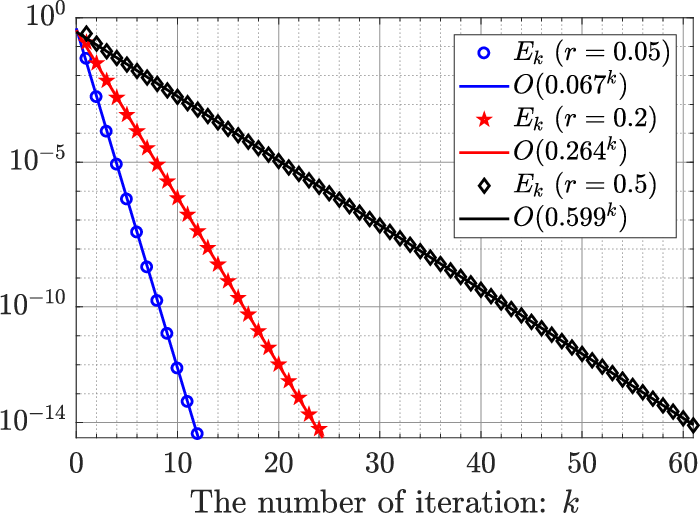
For the parameter $r$ in the above iterative method, in general, the value of $0<r\leq 1$ is chosen such that the inner boundary components are not overlapping, i.e., we need to choose a small value for $r$ if the slits are close to each others. On one hand, the geometry of the preimage domain $G$ will be simpler if we choose $r=1$ or close to $1$ (when it is possible). On the other hand, the rate of convergence of the iterative method depends on the value of $r$ where the method converges faster for small $r$ (see Figure 4 (left) below for the example considered in Section 2.4). However, for small values of $r$, the method requires more GMRES iterations (see Figure 4 (right)). Furthermore, for small values of $r$, the inner boundary components will be thin and hence one needs to consider a larger value of $n$ to achieve a satisfactory accuracy. The preimage domain in Figure 3 is computed with $r=0.2$.

The iterative method presented in the preceding subsection allows us to compute the preimage domain $G$ and the conformal mapping from $z=\Phi(w)$ from $G$ onto $\Omega$. More precisely, it provides us with a parametrization $\eta(t)$, $t\in J$, of the boundary $\partial G$. As described in Theorem 2.1, solving (10) and computing $h$ in (11) permit to determine the boundary values of the auxiliary analytic function $f$. Consequently, the boundary values $\Phi(\eta(t))$ of $\Phi$ can be computed by (12). To determine the values $\Phi(w)$ for $w\in G$, we first compute the values of $f(w)$ using the Cauchy integral formula. In our numerical computations, the values $f(w)$ for $w\in G$ are computed accurately using the MATLAB function fcau presented in Nas-ETNA.

Since $\Phi$ maps $\partial G$ onto $\partial\Omega$, we see that

is a parametrization of $\partial\Omega$, and $\Phi^{-1}(\zeta(t))=\eta(t)$. The boundary of the domain $\Omega$ passes through the point at infinity, which means the Cauchy integral formula cannot be employed to directly compute $\Phi^{-1}(z)$ for $z\in\Omega$. Nevertheless, we write $\Phi^{-1}(z)$ as

where $g=\Phi^{-1}\circ\Psi$ and $\Psi$ is given by (9). The mapping function $\Psi^{-1}$ maps the unbounded domain $\Omega$ onto the bounded domain $\tilde{\Omega}=\Psi^{-1}(\Omega)$ (see Figure 2). The domain $\tilde{\Omega}$ is interior to the unit circle and exterior to $m$ slits (which are not rectilinear) and the boundary of $\tilde{\Omega}$ is parametrized by

The boundary values of $g$ are then given by

For $z\in\Omega$ we have $\tilde{z}=\Psi^{-1}(z)\in\tilde{\Omega}$, and the values of $g(\tilde{z})$ can now be computed using the Cauchy integral formula. Consequently, the values of $\Phi^{-1}(z)$ can be computed through (16), that is,

In the numerical computations presented below, the values of $g(\tilde{z})$ are computed by the MATLAB function fcau. However, to use the function fcau, we need to compute $\tilde{\zeta}^{\prime}(t)$ for $t\in J$ in advance. This derivative is computed by first approximating the real and imaginary parts of $\tilde{\zeta}(t)$ on each sub-interval $J_{j}$, $j=0,\ldots,m$, with trigonometric interpolating polynomials, and then differentiating these polynomials. Note that the interpolating polynomials can be computed by applying the fast Fourier transform Weg05.

All computations in this paper are performed in MATLAB R2017a on an ASUS Laptop with Intel Core i7-8750H CPU @ 2.20GHz, 2208 Mhz, 6 Cores, 12 Logical Processors and 16 GB RAM.

We present a numerical example that illustrates how the iterative method introduced above can be applied to determine the preimage $G$ of an infinite strip with $m=21$ rectilinear slits as shown in Figure 3 (left). The method is applied with $n=2^{11}$ and $r=0.2$ and the obtained preimage domain is displayed in Figure 3 (right). We also compute the error $E_{k}$ defined by (14) and the number of GMRES iterations using $n=2^{11}$ for $r=0.05$, $r=0.2$, and $r=0.5$. The computed error and the number of GMRES iterations vs. the number of iteration $k$ is given in Figure 4. The total CPU time required by the iterative method is $68.91$ sec for $r=0.05$, $70.15$ sec for $r=0.2$, and $127.72$ for $r=0.5$.

We aim to compute the capacity of generalized condensers of the form $C=(S,E,\delta)$ where $S$ is the infinite strip

$E=\{E_{j}\}_{j=1}^{m}$ is a collection of $m$ nonempty closed pairwise disjoint segments $E_{j}=[a_{j},b_{j}]$ with complex numbers $a_{j},b_{j}\in S$, and $\delta=\{\delta_{j}\}_{j=1}^{m}$ is a collection of real numbers. We assume that $m>1$ and $\delta$ contains at least two different numbers. The domain $\Omega=S\setminus E=S\setminus\cup_{j=1}^{m}[a_{j},b_{j}]$ is known as the field of the condenser $C$, the sets $E_{k}$ as the plates, and the numbers $\delta_{k}$ as the levels of the potential of the plates $E_{j}$, $j=1,\ldots,m$ (du, p. 12) (see Figure 5 (left) for $m=4$).

The conformal capacity of the generalized condenser $C$, $\mathrm{cap}(C)$, is given by the Dirichlet integral

where $u$ is the potential function of the condenser $C$, i.e., the function $u$ is the unique solution of the Dirichlet BVP (du, p. 13, p. 305)

If all values of $\delta_{k}$ are equal to $1$ or if $m=1$ (i.e., $E$ consists of only one segment), then $C=(S,E,\delta)$ is a classical condenser and it is shortly denoted by $C=(S,E)$. In this case, the capacity $\mathrm{cap}(C)$ may simply be written as $\mathrm{cap}(S,E)$, see Section 1.

One important property of the capacity of generalized condensers is its invariance under conformal mappings, which implies that domains having complex geometry like $G$ can be treated with the aid of conformal mappings ah; avv; bbgghv; crow-20; dnv; dek; dt; du; et; garmar; hkv; LV; Nvm; Nv; ps; sl; sol; Vas02; vu88; Weg05; wen.

The capacity $\mathrm{cap}(C)=\mathrm{cap}(S,E,\delta)$ will be computed in two steps:
Step 1. For the given domain $\Omega=S\setminus\cup_{j=1}^{m}[a_{j},b_{j}]$, the iterative method proposed in Section 2 will be used to find a preimage domain $G$ interior to the unit circle $\Gamma_{0}$ and exterior to $m$ ellipses $\Gamma_{j}$, $j=1,\ldots,m$. Let $D_{j}$ be the simply connected domain interior to $\Gamma_{j}$ for $j=1,\ldots,m$, let $\hat{E}=\cup_{j=1}^{m}\overline{D}_{j}$, and let $\hat{C}=({\mathbb{D}},\hat{E},\delta)$ (see Figure 5 (right)). Then $\mathrm{cap}(C)=\mathrm{cap}(\hat{C})$.
Step 2. The capacity $\mathrm{cap}(\hat{C})$ will be evaluated by the method that we will describe in the sequel.

We point out that we use the same number $n$ of discretization points for both steps. Now, let us present the method needed in Step 2 to compute the capacity of the generalized condenser $\hat{C}=({\mathbb{D}},\hat{E},\delta)$ where ${\mathbb{D}}$ is the unit disk, $\hat{E}=\{\hat{E}_{j}\}_{j=1}^{m}$ is a family of $m$ nonempty closed and pairwise disjoint sets $\hat{E}_{j}=D_{j}\cup\Gamma_{j}\subset{\mathbb{D}}$, and $\delta=\{\delta_{j}\}_{j=1}^{m}$ is a collection of real numbers. Here, $\Gamma_{j}=\partial\hat{E}_{j}$ is a smooth Jordan curve for $j=1,\ldots,m$. Hence, $G={\mathbb{D}}\setminus\hat{E}$ is a bounded multiply connected domain of connectivity $m+1$, and $\Gamma=\partial G=\cup_{j=0}^{m}\Gamma_{j}$ where $\Gamma_{0}$ is the unit circle and $\Gamma_{1},\ldots,\Gamma_{m}$ are ellipses enclosed in $\Gamma_{0}$ (see Figure 5 (right) for $m=4$).

The above generalized condenser $\hat{C}=({\mathbb{D}},\hat{E},\delta)$ is a special type of the generalized condenser considered in (du, p. 12) and Nvm. Hence, the numerical method presented in Nvm can be used to compute the capacity of the above generalized condenser. For the convenience of the reader, we review this method below.

The conformal capacity of the generalized condenser $\hat{C}$ is

where the potential function $U$ is now the unique solution of the Dirichlet BVP

The harmonic function $U$ is the real part of an analytic function $F$ in $G$ which is not necessarily single-valued. If we take a given point $\alpha_{k}\in G_{k}$ for each $k=1,\ldots,m$, then $F$ can be written as Gak; garmar; Mik64; Mus

where $g$ is a single-valued analytic function in $G$ and $a_{1},\ldots,a_{m}$ are undetermined real constants satisfying (Mik64, §31)

Using Green’s formula (du, p. 4), and in view of (20b)–(20c) and (22), equation (19) can be written as

Consequently, by the conformal invariance of the capacity, we have

The problem (20) above is a particular case of the problem considered in (Nvm, Eq. (4)). Let $\eta(t)$, $t\in J$, be a parametrization of the boundary $\Gamma=\partial G$ and let $A(t)$ be defined (6). Then, the constants $a_{1},\ldots,a_{m}$ in (24) will be computed as in the following theorem from (Nvm, Theorem 4).

The linear system (26) is usually small and can be solved using Gaussian elimination. Henceforth, the capacity can be computed by (24). Note that, in our computation in this paper, we do not need the value of the real constant $c$ in (26).

We now present several examples to illustrate how the above proposed method can be applied to approximate the capacity $\mathrm{cap}(S,E,\delta)$.

The exact value of the capacity of the condenser $(S,E)$ can be given in terms of special functions for this example. For $\Psi$ defined by (9), the mapping function

maps conformally the domain $S\backslash[-s\mathrm{i},s\mathrm{i}]$ onto the domain ${\mathbb{D}}\backslash[-\tan(s/2),\tan(s/2)]$. Then, by the Möbius transformation

the domain ${\mathbb{D}}\setminus[-\tan(s/2),\tan(s/2)]$ is mapped onto the domain ${\mathbb{D}}\setminus[0,\sin(s)]$. Owing to the conformal invariance of the capacity, we have

This yields (see LV, (vu88, Thm 8.6(1))),

where

Here, $\mathcal{K}(r)$ and $\mathcal{K}^{\prime}(r)$ are the elliptic integrals of the first kind, and $\mu:(0,1)\to(0,\infty)$ is a decreasing homeomorphism. For the numerical computation of the values of $\mu(r)$, we use the method described in Nv.

We set $n=2^{10}$ and $r=0.2$ to compute $\mathrm{cap}(S,E)$ for several values of $s$ in $(0,\pi/2)$, and present the numerical results in Table 1. The relative error in the approximate values for $s=0.5$ and $s=1.55$ vs. $n$, the number of discretization points on each boundary component, are depicted in Figure 6 (left). The error is $O(e^{-0.217n})$ for $s=0.5$ and $O(e^{-0.091n})$ for $s=1.55$.

In this case again, the exact value of the capacity of the condenser $(S,E)$ can be determined. Clearly, $z\mapsto\Psi^{-1}(z)=\tanh(z/2)$ maps conformally the domain $S\setminus[-s,s]$ onto the domain ${\mathbb{D}}\setminus[-\tanh(s/2),\tanh(s/2)]$. Then, the Möbius transformation

maps the domain ${\mathbb{D}}\setminus[-\tanh(s/2),\tanh(s/2)]$ onto the domain ${\mathbb{D}}\setminus[0,\tanh(s)]$. Hence, as in the previous example, we have

We now take $n=2^{10}$ and $r=0.2$ to compute $\mathrm{cap}(S,E)$ for several values of $s$. For $s=0.5$ and $s=2$, the relative error in the approximate values vs. $n$ are given in Figure 6 (right). The error is $O(e^{-0.217n})$ for $s=0.5$ and $O(e^{-0.215n})$ for $s=2$.

In this example, we consider the vertical segment $[-\mathrm{i},\mathrm{i}]$ and study the effect of vertically shifting this segment on the capacity of the condenser $(S,E)$. On the left of Figure 7, we display the graph of the capacity $\mathrm{cap}(S,\mathrm{i}s+[-\mathrm{i},\mathrm{i}])$ as a function of $s\in[-0.55,0.55]$. The computation is performed with $n=2^{11}$ and $r=0.1$.

We now consider the horizontal segment $[-1,1]$ and study the effect of vertically shifting this segment on the capacity of the condenser $(S,E)$. The graph of the capacity as a function of $s\in[-1.55,1.55]$, computed using the same parameters as in the previous example, is shown in Figure 7 (right).

By looking at Figure 7, we can notice an increase in the capacity as the segment moves vertically close the boundary of $S$. It is worth noting that horizontal movement of a segment in a strip does not change the capacity value because of translation invariance. In fact, for any segment $[a,b]$ in $S$ and any real number $s$, the linear transformation

maps the domain $S\backslash(s+[a,b])$ onto the domain $S\backslash[a,b]$, and hence by conformal invariance of the capacity, we have

For a given point $a$ in $S$, consider all points $x+\mathrm{i}y\in S\backslash\{a\}$ such that the capacity $\mathrm{cap}(S,[a,x+\mathrm{i}y])$ is constant. The contour lines of the function $\mathrm{cap}(S,[a,x+\mathrm{i}y])$ in the sub-domain $x+\mathrm{i}y\in[-3,3]+\mathrm{i}(-\pi/2,\pi/2)\setminus\{a\}$ are displayed in Figure 8 on the left for $a=0$ and on the right for $a=\mathrm{i}$. For each contour line, we have the same capacity for all segments with one end at $a$ and the other end on the contour line. These results are again computed with $n=2^{11}$ and $r=0.1$.

References

- (1) Ahlfors, L.: Conformal Invariants. McGraw-Hill, New York (1973)
- (2) Anderson, G.D., Vamanamurthy, M.K., Vuorinen, M.: Conformal Invariants, Inequalities and Quasiconformal Maps. John Wiley, New York (1997)
- (3) Aoyama, N., Sakajo, T., Tanaka, H.: A computational theory for spiral point vortices in multiply connected domains with slit boundaries. Japan J. Indust. Appl. Math. 30, 485–509 (2013)
- (4) Baddoo, P., Crowdy, D.: Periodic Schwarz–Christoffel mappings with multiple boundaries per period. Proc. Roy. Soc. A 475, 20190225 (2019)
- (5) Bezrodnykh, S., Bogatyrev, A., Goreinov, S., Grigoriev, O., Hakula, H., Vuorinen, M.: On capacity computation for symmetric polygonal condensers. J. Comput. Appl. Math. 361, 271–282 (2019)
- (6) Crowdy, D.: The Schwarz–Christoffel mapping to bounded multiply connected polygonal domains. Proc. Roy. Soc. A 461, 2653–2678 (2005)
- (7) Crowdy, D.: Schwarz–Christoffel mappings to unbounded multiply connected polygonal regions. Math. Proc. Camb. Phil. Soc. 142, 319–339 (2007)
- (8) Crowdy, D.: A new calculus for two dimensional vortex dynamics. Theor. Comput. Fluid Dyn. 24, 9–24 (2010)
- (9) Crowdy, D.: Solving problems in multiply connected domains. Society for Industrial and Applied Mathematics, Philadelphia (2020)
- (10) Dautova, D., Nasyrov, S., Vuorinen, M.: Conformal module of the exterior of two rectilinear slits. Comput. Methods Funct. Theory 21, 109–130 (2021)
- (11) DeLillo, T., Elcrat, A., Kropf, E.: Calculation of resistances for multiply connected domains using Schwarz-Christoffel transformations. Comput. Methods Funct. Theory 11, 725–745 (2011)
- (12) DeLillo, T., Elcrat, A., Pfaltzgraff, J.: Schwarz-Christoffel mapping of multiply connected domains, J. d’Analyse Math. 94,17–47 (2004)
- (13) Driscoll, T., Trefethen, L.: Schwarz-Christoffel mapping. Cambridge University Press, Cambridge (2002)
- (14) Dubinin, V.: Condenser Capacities and Symmetrization in Geometric Function Theory. Springer, Basel (2014)
- (15) Embree, M., Trefethen, L.: Green’s functions for multiply connected domains via conformal mapping. SIAM Rev. 41, 745–761 (1999)
- (16) Gakhov, F.: Boundary Value Problems. Pergamon Press, Oxford (1966)
- (17) Garnett, J., Marshall, D.: Harmonic measure. Cambridge University Press, Cambridge (2008)
- (18) Greengard, L., Gimbutas, Z.: FMMLIB2D: A MATLAB toolbox for fast multipole method in two dimensions, version 1.2. http://www.cims.nyu.edu/cmcl/fmm2dlib/fmm2dlib.html (2012). Accessed 1 Jan 2018
- (19) Hariri, P., Klén, R., Vuorinen, M.: Conformally Invariant Metrics and Quasiconformal Mappings. Springer Monographs in Mathematics. Springer, Switzerland (2020)
- (20) Lehto, O., Virtanen, K.: Quasiconformal mappings in the plane, 2nd ed. Springer, Berlin (1973)
- (21) Mikhlin, S.: Integral Equations and Their Applications to Certain Problems in Mechanics, Mathematical Physics and Technology, 2nd ed. Pergamon Press, Oxford (1964)
- (22) Muskhelishvili, N.: Singular Integral Equations. Noordhoff, Groningen (1953)
- (23) Nasser, M.: Fast solution of boundary integral equations with the generalized Neumann kernel. Electron. Trans. Numer. Anal. 44, 189–229 (2015)
- (24) Nasser, M.: Numerical computing of preimage domains for bounded multiply connected slit domains. J. Sci. Comput. 78, 582–606 (2019)
- (25) Nasser, M., Al-Shihri, F.: A fast boundary integral equation method for conformal mapping of multiply connected regions. SIAM J. Sci. Comput. 33, A1736–A1760 (2013)
- (26) Nasser, M., Green, C.: A fast numerical method for ideal fluid flow in domains with multiple stirrers. Nonlinearity 31, 815–837 (2018)
- (27) Nasser, M., Kalmoun, E., Mityushev, V., Rylko, N.: Simulating local fields in carbon nanotube reinforced composites for infinite strip with voids. J. Engrg. Math. 134, 8 (2022)
- (28) Nasser, M., Vuorinen, M.: Numerical computation of the capacity of generalized condensers. J. Comput. Appl. Math. 377, 112865 (2020)
- (29) Nasser, M., Vuorinen, M.: Computation of conformal invariants. Appl. Math. Comput. 389, 125617 (2021)
- (30) Papamichael, N., Stylianopoulos, N.: Numerical conformal mapping: Domain decomposition and the mapping of quadrilaterals. World Scientific, New Jersey (2010)
- (31) Sakajo, T., Amaya, Y.: Numerical construction of potential flows in multiply connected channel domains. Comput. Methods Funct. Theory 11(2), 415–438 (2012)
- (32) Schinzinger, R., Laura, P.: Conformal mapping. Methods and applications. Dover Publications, Inc., New York (2003)
- (33) Solynin, A.Yu.: Problems on the loss of heat: herd instinct versus individual feelings. Algebra i Analiz 33(5), 1–50 (2021)
- (34) Vasil’ev, A.: Moduli of Families of Curves for Conformal and Quasiconformal Mappings. Springer-Verlag, Berlin (2002)
- (35) Vuorinen, M.: Conformal geometry and quasiregular mappings. Lecture Notes in Mathematics. Springer-Verlag, Berlin (1988)
- (36) Wegmann, R.: Methods for numerical conformal mapping. In: R. Kühnau (ed.) Handbook of Complex Analysis: Geometric Function Theory, Vol. 2, pp. 351–477. Elsevier B. V. (2005)
- (37) Wegmann, R., Nasser, M.: The Riemann-Hilbert problem and the generalized Neumann kernel on multiply connected regions. J. Comput. Appl. Math. 214, 36–57 (2008)
- (38) Wen, G.: Conformal Mappings and Boundary Value Problems. American Mathematical Society, Providence, RI (1992)