Strategies for Safe Multi-Armed Bandits
with Logarithmic Regret and Risk The bulk of this work was done whilst A.G. was a graduate student at Boston University
Abstract
We investigate a natural but surprisingly unstudied approach to the multi-armed bandit problem under safety risk constraints. Each arm is associated with an unknown law on safety risks and rewards, and the learner’s goal is to maximise reward whilst not playing unsafe arms, as determined by a given threshold on the mean risk.
We formulate a pseudo-regret for this setting that enforces this safety constraint in a per-round way by softly penalising any violation, regardless of the gain in reward due to the same. This has practical relevance to scenarios such as clinical trials, where one must maintain safety for each round rather than in an aggregated sense.
We describe doubly optimistic strategies for this scenario, which maintain optimistic indices for both safety risk and reward. We show that schema based on both frequentist and Bayesian indices satisfy tight gap-dependent logarithmic regret bounds, and further that these play unsafe arms only logarithmically many times in total. This theoretical analysis is complemented by simulation studies demonstrating the effectiveness of the proposed schema, and probing the domains in which their use is appropriate.
1 Introduction
We consider the safety constrained multi-armed bandit problem, where each arm, is modelled by a tuple, consisting of a stochastic reward, of mean and an associated stochastic safety-risk, of mean . Upon playing an arm, the learner observes noisy instances of the reward and safety-risk. The learner is provided with a tolerated risk level, denoted and the goal of the safe bandit problem is to maximise the reward gained over the course of play, while ensuring that unsafe arms—those for which —are not played too often.
We propose the following regret formulation to model the above criteria. Let be the mean reward of the largest safe action, i.e, the largest over arms such that Let be the arm pulled by the algorithm at time . We study
| (1) |
Before describing the results, let us sketch a scenario of particular interest, which informs our formulation.
Clinical Trials. Trial drugs have both positive (eg. curing a disease) and negative side-effects (headaches, nausea, etc) on a patient in a clinical trial, and it is as much in the interest of a patient to ensure that negative side effects are limited as it is to ensure that the drug is effective (Genovese et al. 2013, e.g.). This scenario motivates the problem of choosing drug and dosage (arms) that have the maximum positive response while ensuring that the side-effects remain below some threshold . Since each patient responds differently, the observed response and the manifestation of side-effects for a specific patient can be modelled as random-variables, with the corresponding means representing population averages. Importantly, for such a scenario, safety must be accounted for in a per-round sense - it does no good to alternate between assigning ineffective placebos and effective but harmful doses. Instead we need to ensure that individuals are not exposed to undue risk while accruing benefits.
How does our formulation account for this scenario?
- •
Risk Per Round. Regret ensures that unsafe arms are rarely played in a per-round (per-patient) sense rather than ensuring safety in an overall sense–for any at least one of or must be positive, and so benefits in efficacy due to unsafe dosages are discounted.
- •
Small safety violations are penalized less (smoothness). Small violations of negative side-effects is a permissible risk (elevated nausea level than desired), worth taking on for a few patients, in the hope of finding a drug/dosage that is effective for the population. Our penalty on safety violations is smooth.
- •
Control of Cumulative risk and Violations Since choosing an infeasible arm in any round contributes a constant amount to the regret, a small further ensures that the cumulative safety risk and the cumulative safety violations (i.e. times such that ) are also small.
We next describe our main technical contributions.
Four Optimistic Strategies. We explore doubly optimistic index-based strategies for choosing arms. These maintain optimistic indices for both the reward and safety risk of each arm, and proceed by first developing a set of plausibly safe actions using the safety indices, and then choose the arm with the highest reward index to play, thus encouraging sufficient exploration. In standard bandits there are two broad classes of such index-based strategies - those based on frequentist confidence bounds, and those based on Bayesian posteriors. This suggests four natural variants in the safe bandit case, through two choices for each of the reward and safety indices. We explicitly study three of these - first when both indices are frequentist, second when the safety index is left frequentist but the reward index is replaced by Thompson sampling, and finally when both indices are based on Bayesian methods. While left explicitly unstudied, the case of frequentist reward and Bayesian safety indices follows naturally from our analysis.
Logarithmic Regret Bounds. In all cases, we show that these strategies admit strong gap-dependent logarithmic regret rates. Further each of these also ensure that the number of times any unsafe arm is played at all (i.e., ) is similarly logarithmically bounded. Finally we show a lower bound which demonstrates that our regret bounds are tight in the limit of large time horizons. The proofs adapt existing results of bandit theory to argue that for well designed safety indices, the optimal arm always remains valid, but any unsafe arms are quickly eliminated. Further, so long as remains valid, standard approaches show that inefficient arms cannot be played too often. An interesting consequence is that the play of strictly dominated arms - those that are both unsafe and inefficient - is limited by the larger of the two gaps.
Empirical Results. We complement the above theoretical study with simulations. First, we practically illustrate that prior policy-based approaches to the safe and constrained bandits do not yield favourable play in our scenario. Next, we implement our proposals, and both illustrate that the methods indeed meet the theoretical guarantees, and further contextualise their relative merits in a practical sense. The broad observation regarding the latter is that Thompson sampling based methods tend to offer better performance in terms of means.
1.1 Related Work
Bandit problems are exceedingly well studied, and a plethora of methods with subtle differences have been established. We refer the reader to the recent book of Lattimore & Szepesvári 2020 for a thorough introduction.
We first describe prior approaches to constrained bandit problems from a formulational point of view. The most important aspect of this is that prior formulations tend to constrain play in an aggregate sense. This raises issues when we need to ensure safety in a per-round sense, as is illustrated by a running example. We then contextualise our methodological proposals with respect to the prior work, and finally discuss pure exploration in the safe-bandit setting.
Globally Constrained Formulations The theory of bandits with global constraints was initiated by Badanidiyuru et al. 2013, and extended by Agrawal & Devanur 2014. Specialised to our context, these works constrain the total number of adverse effects whilst matching the performance of the optimal dynamic policy that is aware of all means. More concretely, suppose that the safety risk observed is a random variable . Badanidiyuru et al. 2013 enforce the hard constraint that while Agrawal & Devanur 2014 relax this into a second regret and ensure that this is small.
Such aggregate safety formulation is lacking from our perspective, as is illustrated by the following simple example of two arms with means
| (2) |
Due to the global constraint, the optimal dynamic policy is to pull arm for rounds, and then switch to pulling arm . A low regret algorithm must then also pull arm times. However, such play undesirably exposes a linear number of rounds to the very unsafe action . Our formulation instead would penalise every play of arm by a cost of and thus effective schema would only play arm sublinearly many times. It should be noted that since the constraint is applied in a per-round way, the optimal dynamic policy in our case is supported on a single arm.
In passing, we also mention the conservative bandit problem (Wu et al. 2016), which only considers rewards, and enforces a running aggregate constraint that for any round , . While an interesting variation, we note that such a running constraint on safety-risk would have similar issues as the above in our situation.
Per-round Constraints The recent work of Pacchiano et al. 2021 studies the safe bandit problem with two crucial differences from us. Firstly, the action space is lifted from single arms to policies (i.e. distributions) over arms, denoted , and secondly, the hard per-round constraint is enforced. Of course, actual arms are selected by sampling from . The regret studied is where is the optimal static safe policy, i.e., the maximiser of subject to Exploration is enabled by giving the scheme an arm known a priori to be safe, and by spending the slack as room for exploration in .
While ostensibly constrained at each round, this formulation suffers from similar issues as the previously discussed globally constrained formulations since the optimal static policy is only safe in aggregate. Indeed, in the previous example (2), the optimal is and so a low regret algorithm must place large mass on the unsafe arm in most rounds, therefore exposing about rounds to it.
A similar approach, but crucially without the policy action space, was taken by Amani et al. 2019; Moradipari et al. 2021 for in the linear bandit setting. These papers also study hard round-wise safety constraints, and again utilise a known safe action, as well as the continuity of the action space to enable sufficient exploration. We note that the particulars of the signalling model adopted by Amani et al. 2019 paper preclude extending their results to the multi-armed setting, and while the model of Moradipari et al. 2021 does admit such extension, the scheme proposed fundamentally relies on having a continuous action space with a linear safety-risk, and cannot be extended to multi-armed settings without lifting to policy space.
Methodological Approaches The bulk of the previous papers are based on frequentist confidence bounds, with two variants. Similar to our Alg. 1, Agrawal & Devanur 2014 use doubly optimistic methods that maintain optimistic upper bounds on the rewards and lower bounds on the risk, and play the policy that maximises reward upper bounds while being safe with respect to the risk lower bounds. In contrast, Pacchiano et al. 2021; Amani et al. 2019; Wu et al. 2016 all use optimistic-pessimistic methods, which instead maintain upper bounds on both the rewards and safety risk and play the actions with maximum reward upper bound whilst being safe with respect to the stringent risk upper bounds. Moradipari et al. 2021 take a similar pessimistic approach, but replace the reward upper bounds with a Thompson sampling procedure that is similar in spirit to our Alg. 2, although this uses optimistic safety indices. We also further study a fully Bayesian approach in Alg. 3.
Pure Exploration with Safety Katz-Samuels & Scott 2018; Katz-Samuels & Scott 2019 design procedures for finding the best feasible arm based on a combination of optimistic and pessimistic confidence bounds that is typical of pure exploration approaches. An interesting variant of this problem was studied in a recent preprint of Wang et al. 2021, who associate a continuous ‘dosage’ parameter with each arm, now interpreted as a single drug, with the understanding that both reward and risk grow monotonically with dosage. These should be compared to the dose-finding bandit problem Aziz et al. 2021, which seeks to identify a dose level out of options that minimises with the intuition being that higher doses are more effective, and so should be maximised, but without exceeding the safety threshold by much. The dose-finding approach relies strongly on this assumed monotonicity. This models the scenario of a single drug, but is inappropriate for the setting of multiple drugs that are trialled together, which is better represented as a constrained optimisation problem (as studied by the former papers). Our formulation takes precisely this view, but from the perspective of controlling regret rather than identification. Note that our smooth penalty for safety violation, bears similarities to the absolute value loss where again a small violation of safety is not penalised strongly.
2 Definitions and Setup
An instance of the safe bandit problem is defined by a risk level a natural , corresponding to a number of arms, and a corresponding vector of probability distributions, each entry of which is supported on We will represent the corresponding random vector as two components which are termed the reward and safety-risk of a draw from . We further associate two vectors corresponding to the mean reward and safety-risk of each arm, i.e
and need not be independent - this has little effect on the subsequent study, since each is marginally bounded.
The scenario proceeds in rounds, denoted . At each , the learner (i.e. an algorithm for the bandit problem) must choose an action corresponding to ‘pulling an arm.’ Upon doing so, the learner receives samples independently of the history. The learner’s information set at time is and the action must be adapted to the filtration induced by these sets. The learner is unaware of any properties of the laws beyond the fact that they are supported on .
The competitor, representing the best safe arm given the safety constraint and the mean vectors, is defined as
and its mean reward and safety risk are denoted as . We will use this convention throughout - for any symbol we set We can ensure that the problem is feasible by including a no-reward, no-risk arm of means - this might correspond to a placebo in a clinical trial. Without loss of generality, we will assume that is unique. We define the inefficiency gap and the safety gap of playing an arm as
where and we will also use . Note that for .
The performance of a learner for the safe bandit problem is measured by the (pseudo-) regret of (1), which may also be written as
Further, with each arm , we associate state variables denoting the number of times it has been played up to time , and denoting the total rewards and safety risk incurred on such rounds. More formally,
Similarly, denote the corresponding variables for . Notice that We also use the notation .
Since controlling it is of natural interest, we define the number of times an unsafe arm is played as
Finally, for we use the notation
to denote the KL divergence between Bernoulli laws with means and We will also need the notation
Remark While the formulation focuses on a single safety-constraint, this may be extended. For example, we may posit a safety-risk vector , and demand that the corresponding (vector) means should lie in some known safe set Natural extensions of the methods below would control, e.g., We focus on a single constraint for clarity and ease of exposition.
3 Doubly Optimistic Confidence Bounds
The use of optimistic confidence bounds is well established in standard bandits (Lattimore & Szepesvári 2020, e.g. Ch. 7-10). The idea is that pulling according to the maximum optimistic bound on the means encourages exploration, while efficiency follows because the confidence bounds exploit information to shrink towards the means, eventually giving evidence for the inefficiency of suboptimal arms.
The idea behind doubly optimistic bounds is identical - we maintain lower bounds on safety-risk and upper bounds on rewards such that and with high probability. We then construct a set of ‘permissible arms’ - these are all the arms that are plausibly feasible given the information we have up to time . is selected to maximise amongst . The optimism of allows us to explore for high rewards, but the concentration of as grows serves to identify unsafe arms, which then cease to be pulled. The broad scheme is described in Algorithm 1.
This scheme can be analysed using a variation of the standard bandit analysis. To control the play of unsafe arms, we argue that is bounded as . Thus, if the arm should fall out of after it has been played at most times. Next we argue that the bounds are ‘consistent’ (or optimistic) with high probabiliy, that is, most of the time and . Given this, in order to play arm , must exceed but shrinks as bounding as . In the process, strictly dominated - for which and are doubly penalised, and their play is limited by the larger gap.
We will explicitly analyse the scheme by instantiating the method with bounds based on KL-UCB (Garivier & Cappé 2011), which offer optimal mean-dependent regret control for standard bandits. Note that the study of confidence bounds for bandit methods is mature, and our results can be improved with other choices of such bounds, e.g. , using variance sensitive bounds such as Empirical-KL-UCB (Cappé et al. 2013) or UCBV (Audibert et al. 2009).
The KL-UCB type bounds take the following form
where trades-off the width and consistency of . These bounds are natural for Bernoulli random variables, and since these are the ‘least-concentrated’ law on the fluctuation bounds extend to general random variables. Using these, we show the following result in §B.1.
Theorem 1.
Algorithm 1 instantiated with KL-UCB type bounds attains the following for any and any
where . Further, the number of times an unsafe arm is played is bounded as
The in the above hides instance-dependent constants, the most pertinent of which is a dependence on with the term. To ameliorate this, we also give a gap-independent analysis of the scheme in §B.2.
Theorem 2.
Algorithm 1 instantiated with KL-UCB attains
The above statement extends to KL-UCB for standard bandits upon sending , which, surprisingly, appears to have been unobserved, at least explicitly.
4 Bayesian Methods
Thompson Sampling (TS) is the first proposed method for bandit problems (Thompson 1933), and encourages exploration by using randomisation. The idea is to choose an benign prior, and play arms according to their posterior probability being optimal. The posteriors remain flat for insufficiently explored arms, giving a non-trivial chance of pulling them. An advantage of TS lies in the fact that it exploits a posterior that may be much better adapted to the underlying law than confidence bounds that rely on a few simple statistics. Indeed, it has been empirically observed that TS offers improved regret versus comparable UCB methods in multi-armed bandits (Chapelle & Li 2011).
This section explores the use of Bayesian methods for safe bandits. We start by replacing the KL-UCB based selection of arms to play in Algorithm 1, but retaining the construction of . We then study a Bayesian method of selecting
In the subsequent, we restrict analysis to the case of Bernoulli bandits, i.e., where the laws are such that marginally and We note that since the resulting bounds depend on only the means of the rewards and safety-risk, these bounds extend to generic laws supported on - indeed, as observed by Agrawal & Goyal 2012, one can exploit an algorithm for Bernoulli bandits for generic laws by passing to the algorithm two samples . The corresponding are then Bernoulli with the same means, and any guarantee that only depends on the means for the Bernoulli case extends to the underlying bandit problem. Of course, such a procedure may blow up variances, and thus be profligate in the case of highly concentrated instances.
Note: the methods described below admit essentially the same guarantees as the bounds of Theorems 1 and 2. For the sake of brevity, we suppress the explicit bounds on and the gap-independent bounds in the following.
4.1 Thompson Sampling with Optimistic Safety Indices
For Bernoulli bandits, it is natural to use the family for priors, due to favourable conjugacy. The standard form of TS instantiates each arm with the uninformative prior The corresponding posterior at time is .
Algorithm 2 describes the proposed strategy - we retain the optimistic lower bound from Algorithm 1, but replace the arm selection given to a TS strategy: random scores are drawn from the posterior for each arm in the arm with the largest is pulled.
The analysis of such a method is simple, given an analysis of TS for standard bandits. Indeed, we can control the play of infeasible arms as we did for Algorithm 1. Further, as long as we can ensure with high probability, we can invoke the decomposition
The first term is handled using the consistency of the lower bound . The second term is essentially the term analysed for standard bandits, and we can use any analysis of TS to control it. We concretely use the approach of Agrawal & Goyal 2013 in §C to show the following result.
Theorem 3.
For Bernoulli Bandits, Algorithm 2 instantiated with a KL-UCB type confidence bound attains the following regret bound for any and any
where
4.2 Thompson Sampling with BayesUCB
While Algorithm 2 admits a tight analysis, it still uses the potentially loose frequentist bound to decide and it is possible that using the posteriors on the safety-risks to do this may improve the behaviour.
It is tempting to appeal to the basic structure of Thompson sampling, and associate a posterior with the safety risk of sample safety scores and let However, this attempt is misguided, essentially because we need to compare the scores to a fixed level rather than amongst each other. Indeed, if it is the case that then there is a constant chance that even if the empirical mean is faithful. This would mean a constant chance of playing a suboptimal arm, and so linear regret. A similar issue has been observed with trying to analyse TS using the analysis developed for UCB-type schema (Kaufmann et al. 2012b), but the issue is now at the level of the scheme rather than an analysis. Indeed, we show via simulations that when such a scheme suffers linear expected regret (§F.4).
So, this idea needs a fix. One natural attempt is to introduce a slack, say some such that . This should likely decay as rises, but be large enough to ensure that - this is similar to the analytical approach taken by Kaufmann et al. 2012b. However, in designing such a we are functionally designing a confidence bound, somewhat defeating the purpose.
We take a different tack, and instead use a Bayesian confidence bound, essentially exploiting the BayesUCB method of Kaufmann et al. 2012a. The idea is to choose a th quantile of the posterior as a score, where is a schedule that decays with . This is able to exploit the potentially improved adaptivity of the posterior, but due to being small, would continue to produce an optimistic score, and so have a high chance of at any time. Additionally, due to the concentration of the -law for large the score of unsafe arms would converge towards and thus preclude their play beyond a point. Altogether, the method seems tailor-made for our situation of filtering arms at a given level. The scheme is described in Algorithm 3, where denotes the th quantile of the law . We introduce a slight bias in the same for technical convenience.
The main design parameter is which trades off the consistency and tightness. In our argument, we use a conservative choice of which leads to a simplified proof, but introduces the inefficiency of in the bounds below. We find that in simulations, the uniform choice is better (§F.3), and perhaps an improved analysis can establish better bounds for such a schedule. The following summarises our analysis in §D.
Theorem 4.
For Bernoulli bandits, Algorithm 3, instantiated with attains the following regret bound for any and any
where
5 Lower Bound
We conclude our theoretical study with a lower bound for algorithms that admit sub-polynomial regrets against all bounded distributions. This is based on the technique of Garivier et al. 2019, who use the chain rule of KL divergence and the data processing inequality to show the following relation, which extends to our case without change:
Lemma 5.
For any safe bandit algorithm, and any two safe bandit instances and any ,
This lemma enables a standard approach - pick so that , and leave the other s unchanged. For any bandit algorithm with sub-polynomial mean regret, the right hand side grows as while the left hand side side reduces to . Of course, the optimal choice of depends subtly on the details of We study a simple concrete case to illustrate that our prior analyses are tight.
Proposition 6.
Any algorithm that ensures that, uniformly over all instances of safe Bernoulli bandit problems with independent rewards and safety-risks, the mean number of plays of any suboptimal arm is bounded as for every must satisfy
Since mean regret can be expressed in terms of this also lower bounds regret. Note the sum in the denominator, rather than a max as in our upper bounds. This means that for strictly dominated arms (i.e. ), our scheme may be loose by up to a factor of two. This arises since our scheme does not utilise the dependence structure of and represents an opportunity for future work.
6 Simulations
We provide practical contextualisation for the schema described in the theoretical section using simulation studies over small safe bandit environments. Of course, to concretely study the schema we describe, we need to instantiate them with appropriate confidence bounds. We will do so using the KL-UCB and BayesUCB based indices which we analysed previously. Finally, we use TS instantiated with the Beta priors as described in the text. Of course, a variety of other methods can be implemented in these schema, but we believe that these methods serve well to illustrate both the theory and a first order practical design. All implementation details are left to §F.
We will begin by empirically illustrating that the prior policy based methods are indeed ineffective in our scenario, and play unsafe arms far too often. We then illustrate the performance of the methods on a realistic problem instance. Finally, we will and investigate the dependence of regret of the three methods on the gaps to the optimal arm.
6.1 Empirical Demonstration of the Ineffectiveness of Prior Formulations
As discussed previously, the globally constrained (Badanidiyuru et al. 2013; Agrawal & Devanur 2014) and policy level (Pacchiano et al. 2021) formulations are unsatisfactory in the context of safety-constraints, as illustrated by example (2). Nevertheless, a priori it may be possible that the schema designed for these objectives may be effective in our scenario, especially if there exist optimal policies supported on a single arm. We implement the the doubly optimistic policy method (BwCR) of Agrawal & Devanur 2014, and the optimistic-pessimistic method (Pess) of Pacchiano et al. 2021 to demonstrate that this is untrue.
We explore two illustrative cases, both of which are for Bernoulli bandits with independent means and safety-risks. The data reported is across trials of horizon . Since these policy methods are based on confidence bounds, we also compare them to Alg. 1. In all cases we instantiate these schema with KL-UCB-based confidence bounds.
1. Multiple optimal policies. We consider four arms with
The arm is included as a known safe arm, which is required for Pess to enable sufficient exploration. Notice that in this case there are two optimal static policies - one that is entirely supported on arm , while another that is uniformly supported on arms and . However, which one of these two policies these schema converge to is essentially random, and we thus see linear growth of in Fig. 1.
2. Single arm optimal policy. We jack up the rewards of arm to but leave the other means unchanged. Now the optimal policy is singly supported on arm and has a significant gap of . Despite the fact that such a case is the most promising for policy-based methods in terms of efficacy in our formulation, Fig. 1 again shows that they do rather poorly - for instance, while our implementation play the unsafe arms about 550 times, these methods play it at least 8000 times. This occurs because the policy-based methods are designed for the much richer policy space—a simplex—and so must explore a lot more than methods designed for single arm play. We note that in this case, while BwCR plays unsafe arms more often, it suffers less regret than Pess, since the unsafe arm incurs a smaller loss.


6.2 Characterisation of the Proposed Schema
We implement the three methods to establish a practical contextualisation of their performance, and to verify the theoretical claims. For the sake of realism, we use the data of Genovese et al. 2013, who report efficacy and infection rates from a phase 2 randomised trial for various dosages of a drug to treat rheumatoid arthritis. The dosages studied were mg, and the observations were
This data is challenging for any safety level - no matter the choice, we have to deal with either a potential safety gap of order , or an efficacy gap of , both of which contribute a large regret. We study the safety level under which arm is optimal, while arms are unsafe. We chose this to allow large enough safety gaps that the behaviour of is easy to establish with runs of length about - if we took smaller, say then we would expect to need runs of length simply to reach a point at which arm is played fewer than about a third of the time. This consideration also illustrates why the regret is a much more reasonable notion of study than which can grow very large due to tiny, practically undetectable safety gaps. Plots for a run with are included in §F.2.


Observations of Performance From Fig.2, we first note that both and are well controlled and well within the theoretical bounds for the methods we have analysed.11 1 The main term of the regret bound is and the unsafe-arm bound is both for . The general trend observed is that Alg. 2 based methods that use a TS-based index outperform confidence bound indices of Alg. 1, which is consistent with Chapelle & Li 2011. Finally, we observe that Alg. 3, as represented by TS+BayesUCB outperforms all other methods. These observations held regardless of the means we have run the methods on. One caveat, however, is that the underlying Bernoulli laws used are well aligned to the priors for Bayesian methods, which may improve their performance.
6.2.1 Dependence on Gaps
We investigate the dependence of the regret on the gaps , in particular illustrating that, as predicted by the theorems, this decays inversely with the larger of the two, and is insensitive to the smaller of the two.
Inverse Dependence on Gaps First, we will demonstrate that the regret varies with inversely. To this end, we study the the cases
for over in over trials across a horizon of Fig. 3 reports the regret versus over this data, and exhibits a clear inverse dependence on .
Lack of Dependence on Smaller Gaps Secondly, we will illustrate that the dependence on the gaps is driven by the larger of and , but not on . For this we study the data
again with for trials over a horizon of . Observe that is the same as the previous case, but is reduced by a factor of for each suboptimal arm. The principal observation from the second part of Fig. 3 is that the plot remains similar to the previous case of ‘large’ minimum gaps, bearing out this independence from the smaller of the two gaps.


References
- Agrawal & Devanur (2014) Agrawal, S. and Devanur, N. R. Bandits with concave rewards and convex knapsacks. In Proceedings of the fifteenth ACM conference on Economics and computation, pp. 989–1006, 2014.
- Agrawal & Goyal (2012) Agrawal, S. and Goyal, N. Analysis of Thompson sampling for the multi-armed bandit problem. In Conference on learning theory, pp. 39–1. JMLR Workshop and Conference Proceedings, 2012.
- Agrawal & Goyal (2013) Agrawal, S. and Goyal, N. Further optimal regret bounds for Thompson sampling. In Artificial intelligence and statistics, pp. 99–107. PMLR, 2013.
- Amani et al. (2019) Amani, S., Alizadeh, M., and Thrampoulidis, C. Linear stochastic bandits under safety constraints. In Advances in Neural Information Processing Systems, volume 32, 2019.
- Audibert et al. (2009) Audibert, J.-Y., Munos, R., and Szepesvári, C. Exploration–exploitation tradeoff using variance estimates in multi-armed bandits. Theoretical Computer Science, 410(19):1876–1902, 2009.
- Aziz et al. (2021) Aziz, M., Kaufmann, E., and Riviere, M.-K. On multi-armed bandit designs for dose-finding clinical trials. Journal of Machine Learning Research, 22:1–38, 2021.
- Badanidiyuru et al. (2013) Badanidiyuru, A., Kleinberg, R., and Slivkins, A. Bandits with knapsacks. In 2013 IEEE 54th Annual Symposium on Foundations of Computer Science, pp. 207–216. IEEE, 2013.
- Cappé et al. (2013) Cappé, O., Garivier, A., Maillard, O.-A., Munos, R., and Stoltz, G. Kullback-leibler upper confidence bounds for optimal sequential allocation. The Annals of Statistics, pp. 1516–1541, 2013.
- Chapelle & Li (2011) Chapelle, O. and Li, L. An empirical evaluation of Thompson sampling. Advances in neural information processing systems, 24:2249–2257, 2011.
- Garivier & Cappé (2011) Garivier, A. and Cappé, O. The KL-UCB algorithm for bounded stochastic bandits and beyond. In Proceedings of the 24th annual conference on learning theory, pp. 359–376. JMLR Workshop and Conference Proceedings, 2011.
- Garivier et al. (2019) Garivier, A., Ménard, P., and Stoltz, G. Explore first, exploit next: The true shape of regret in bandit problems. Mathematics of Operations Research, 44(2):377–399, 2019.
- Genovese et al. (2013) Genovese, M. C., Durez, P., Richards, H. B., Supronik, J., Dokoupilova, E., Mazurov, V., Aelion, J. A., Lee, S.-H., Codding, C. E., Kellner, H., et al. Efficacy and safety of secukinumab in patients with rheumatoid arthritis: a phase ii, dose-finding, double-blind, randomised, placebo controlled study. Annals of the rheumatic diseases, 72(6):863–869, 2013.
- Jeřábek (2004) Jeřábek, E. Dual weak pigeonhole principle, boolean complexity, and derandomization. Annals of Pure and Applied Logic, 129(1-3):1–37, 2004.
- Katz-Samuels & Scott (2018) Katz-Samuels, J. and Scott, C. Feasible arm identification. In International Conference on Machine Learning, pp. 2535–2543. PMLR, 2018.
- Katz-Samuels & Scott (2019) Katz-Samuels, J. and Scott, C. Top feasible arm identification. In The 22nd International Conference on Artificial Intelligence and Statistics, pp. 1593–1601. PMLR, 2019.
- Kaufmann et al. (2012a) Kaufmann, E., Cappé, O., and Garivier, A. On bayesian upper confidence bounds for bandit problems. In Artificial intelligence and statistics, pp. 592–600. PMLR, 2012a.
- Kaufmann et al. (2012b) Kaufmann, E., Korda, N., and Munos, R. Thompson sampling: An asymptotically optimal finite-time analysis. In International conference on algorithmic learning theory, pp. 199–213. Springer, 2012b.
- Lattimore & Szepesvári (2020) Lattimore, T. and Szepesvári, C. Bandit algorithms. Cambridge University Press, 2020.
- Moradipari et al. (2021) Moradipari, A., Amani, S., Alizadeh, M., and Thrampoulidis, C. Safe linear Thompson sampling with side information. IEEE Transactions on Signal Processing, 2021.
- Pacchiano et al. (2021) Pacchiano, A., Ghavamzadeh, M., Bartlett, P., and Jiang, H. Stochastic bandits with linear constraints. In International Conference on Artificial Intelligence and Statistics, pp. 2827–2835. PMLR, 2021.
- Thompson (1933) Thompson, W. R. On the likelihood that one unknown probability exceeds another in view of the evidence of two samples. Biometrika, 25(3/4):285–294, 1933.
- Wang et al. (2021) Wang, Z., Wagenmaker, A., and Jamieson, K. Best arm identification with safety constraints. arXiv preprint arXiv:2111.12151, 2021.
- Wu et al. (2016) Wu, Y., Shariff, R., Lattimore, T., and Szepesvári, C. Conservative bandits. In International Conference on Machine Learning, pp. 1254–1262. PMLR, 2016.
Appendix A Notation and Broad Proof Strategy
We begin with some notation, and then describe the general proof strategy.
We will abuse notation and let also stand for the sigma algebra induced by the history, with denoting the trivial sigma algebra. Naturally, forms a filtration - observe that in the TS cases, the laws of are measurable with respect to . The Bayesian methods also utilise extraneous randomness, as represented by the various s. An important observation regarding all the methods we design is that the permissible set is a predictable process, i.e., is determined given . Indeed, all the methods use an index based on the history to decide and so it is a deterministic function of the variables Of course, this is not as such required, but it represents a convenience that we will employ in our proofs. For the sake of brevity, we will denote the conditional laws as .
Proof strategy The basic decomposition of regret is in terms of - indeed, due to the additive definition,
Therefore, the main arguments all control for all suboptimal arms . Of course, subsidiary claims about also follow from these.
The arguments separately control for infeasible and inefficient arms. For arms which are both inefficient and infeasible, the tighter of the control offered by these two arguments can be taken, and this yields the form of the expressions in the main text.
Infeasible arms All of our schemes use a safety index to populate the permissible set . We exploit the properties of this index to control the play of infeasible arms. Indeed, we can decompose
The design of the two indices - that via KL-UCB and via BayesUCB both ensure that the chance of playing an infeasible arm more than times is exponentially small. For KL-UCB, this is a simple consequence of Chernoff’s bound. For BayesUCB, the argument reduces to that for KL-UCB using a connection between the tails of Beta distributions and Binomials.
Inefficient arms Following the standard method for confidence bound based index policies, controlling the play of inefficient arms requires some known good index to compare the reward indices to. Naturally, we want to use the index of but doing so requires that itself is permitted, since otherwise the algorithm never takes its reward index into consideration when choosing an arm. This represents the main deviation from standard proofs.
Let us take the case of KL-UCB. The idea is to decompose
The first course of action then is to ensure that the first term is small, which exploits the consistency of .
This enables us to proceed pretty much as usual. For KL-UCB, we decompose the second term as
Of course, the final expression is the usual quantity controlled in regret proofs, and this argument can be repeated without change. For the sake of being self-contained, we will sketch these proofs in the subsequent as well. For KL-UCB, this is essentially the argument of Garivier & Cappé 2011, while for the BayesUCB bound, this is the argument of Kaufmann et al. 2012a (which itself is very similar to Garivier & Cappé 2011). For the efficiency of TS, we will use the argument of Agrawal & Goyal 2013.
Remark on showing consistency of We observe that, by design, our choices of are such that consistency proofs for translate directly into those for - this is due to the symmetry of the relevant functionals under the maps upon doing which is a -type upper bound for . Similarly, the argument for controlling for infeasible arms is basically the same as that for controlling for the standard bandit version of the appropriate method.
That said, we note a deviation from the proof of this consistency for the case of BayesUCB. Since controlling standard regret in a Bayesian setting requires one to compare two random indices, Kaufmann et al. 2012a use direct comparison of their index to only enough to argue that is at least logarithmically large. With this in hand, they can argue that is at least with high probability and argue that this is unlikely to be exceeded by suboptimal arms. However, to ensure that our (random) safety index is consistent, we must compare it to a fixed value , and so this second argument utilising a weakened consistency does not carry over. We handle this by loosening the quantiles enough so that the first argument itself is sufficient to provide consistency. This represents a gap, which may be possibly be resolved by a stronger analysis.
Remark on dependence Note that the sketch above above does not use the potential dependence between the signals It is possible that this can be exploited, and this exploitation may gain in importance as we increase the number of safety constraints. We leave this as a direction for further work.
Appendix B Proof for Doubly Optimistic Confidence Bounds
The following lemma essentially follows from the main result of the KL-UCB analysis due to Garivier & Cappé 2011, and forms the key statement to demonstrate our results. We note that this is stated slightly more generically than in their paper, essentially to let us use the same result to show both gap dependent and gap independent bounds. We came across this trick in the work of Agrawal & Goyal 2013.
Lemma 7 (Adaptation of Garivier & Cappé 2011).
Let be a suboptimal arm. Then Algorithm 1, instantiated with the KL-UCB type confidence bounds attains the following guarantees for all .
- •
If then for any
(3) - •
If then for any
(4)
We will first show the proofs of the two results using the above lemma, and leave proving it until the end.
B.1 Proof of Theorem 1
Proof.
Fix an arm . If then choose such that - this exists since is continuous and monotonically decreases from to as varies in We need to argue that the third term in the bound of (3) is bounded as . This follows since for small .
Indeed, let us abbreviate and observe that the the derivative is non-zero, and so But then notice that since is minimised at where . We conclude that
which of course is a scaling of by a problem dependent constant.
Next, if we proceed similarly to the above, and choose such that By an entirely identical calculation as above, the final term of (4) is bounded as where and
Using both of these bounds, we conclude that
where we set when the proposition is untrue. Of course, recalling that and similarly we may choose the tighter of the above bounds to get the result
The claimed bounds now follow trivially - to control simply multiply by the per-round regret of playing arm , and sum. To control simply add up the above over the unsafe arms.
∎
Note that as the gaps and decay, the last term scales as , which only yields a gap-independent bound.
B.2 Proof of Theorem 2
As is standard, the gap-independent regret bounds follow on observing that arms for which the gap is too small cannot actually incur large regret over rounds. To this end, let be a parameter to be chosen, and express regret as
| (5) |
The last term is of course bounded by and so we will end up taking of order to control regret. It remains to show that is not too large for arms with large gaps. To this end, we first develop bounds dependent explicitly on the gaps using (3) and (4).
Lemma 8.
For any arm with
Similarly, for any arm with
Proof.
First, take a with and in the bound (3), set By Pinsker’s inequality, and Plugging these into the bound yields the claim upon observing that
For arms with we can develop a similar control resulting from by setting . ∎
We are now in a position to show the claim.
B.3 Proof of Lemma 7
Proof.
We make the argument separately for infeasible and inefficient arms. The former is easier, so let us begin with it.
Infeasible arms
We follow the decomposition from §A. Recall that . Since is a continuous decreasing function on if then it must either hold that or Either way, we have that .
Now, let denote the value of after the th time we play the arm . We observe that
where we have used that increases with , and for any value , there is at most one time step on which is exactly and we play the action .
Now, we observe that for any the event Indeed, is exactly equal to for and monotonically increasing for . But, recalling Chernoff’s bound (which applies since the random variables are bounded in ), This sets up the following calculation.
Let and define so that for all . Then
| (6) |
where the last term uses that , and But
As noted in §A, the final term is controlled in exactly the same way as the inefficiency control. Indeed, . Since increases in the range if then either or . Developing the subsequent bound in exactly the same way, we find that
and again, for any The resulting sum then gives the bound
where
It remains to control . To control the second term, we first exploit the monotonicity of on to note that
The final event is the subject of (Garivier & Cappé 2011, Theorem 10,), who show that for any , and any
| (7) |
The statement extends, of course, to the empirical mean of any subsampling of any i.i.d. process in . The gist of the argument is to partition the space according to the size of . If is non-trivially large at some fixed time , then it is exponentially unlikely for to exceed , essentially because the cumulant generating function is bounded by that of a Bernoulli, and is the Fenchel dual of this function for the Bernoulli. It is then just a question of stitching together these bounds over a well-chosen grid of values that may take (concretely, a geometrically increasing grid is used, and we end up with a due to this grid), and accounting for the poor behaviour for small (whence the premultiplying ). The argument presented in the supplement to the follow up work by Cappé et al. 2013 is somewhat cleaner than the original, and might be preferred.
Putting these together, we have
where we have used . ∎
Appendix C Proofs for Thompson Sampling with Optimistic Safety Indices
The first observation is that since the safety index remains unchanged, we may directly use the proofs of Lemma 7 to observe that the bounds and (9) continue to hold, that is,
The focus of the study then is to ensure that the TS analysis extends to control the play of inefficient arms. This pretty much exploits the analysis of TS due to Agrawal & Goyal 2013, although alternate analyses such as that of Kaufmann et al. 2012b can equivalently be used.
The main bound is summarised in the following
Lemma 9 (Adaptation of Agrawal & Goyal 2013).
There exists a universal constant such that if then for any such that ,
| (10) |
Let us first demonstrate the result from the main text using the above Lemma.
Proof of Theorem 3.
We first argue the theorem.
For infeasible arms, instantiate (4) with a such that . Since as previously argued, the resulting is
For inefficient arms, consider the decomposition
The first term is bounded as For the second term, we instantiate the bound (10) with a and a chosen so that
- 1.
- 2.
both of which exist by continuity.
Showing the bound then requires control on and (using the upper bound ). To this end, as in the proof of Theorem 1, observe that Similarly, Therefore, Finally, since this term does not grow with , .
We may now conclude the argument exactly as in the proof of Theorem 1 ∎
Similarly to the case for Algorithm 1, this scheme also admits a gap-independent bound.
Proposition 10.
Algorithm 2, instantiated with KL-UCB type lower confidence bounds, attains the gap independent regret bound
Proof.
For infeasible arms, instantiate (4) with to conclude that
For inefficient arms, instantiate (10) with and Then and by observing that we have the upper bound
Taking the tighter of these bounds, and partitioning according to the size of , we have the bound
giving the claim upon optimisation. ∎
It remains to show the key Lemma. Again, we note that the key ideas are due to Agrawal & Goyal 2013.
Proof of Lemma 9.
Fix a . The values and essentially represent indices that we can compare the random scores and to. To this end, we define the ‘good’ events
Notice that lies in .
Now, we start with the decomposition
| (11) |
Now, the last of these terms in (C) is easily controlled - indeed, is exponentially small if is large. In fact, mirroring the approach of the proof of Lemma 7, we find that
where we set to be the value of at the first such that . But then, by Chernoff’s bound, giving the bound
| (12) |
The second term of (C) too is similar to control, upon observing that the posterior law is very well concentrated around with variance scale More concretely, Agrawal & Goyal 2013 exploit the following observation: if is the CDF of a random variable, and is the CDF of a Binomial random variable, then for natural
This relation most easily follows from the fact that the is the law of the th order statistic of samples from the uniform distribution, and the chance of this exceeding is simply the chance that the smaller ones are at most , and the rest are at least , which of course is expressed by the Binomial distribution. But then we conclude that for any
Choosing we then get the bound
| (13) |
This leaves the first term of (C), which is the hardest to control, and ultimately relies upon hard analysis of Binomial tails. The idea is roughly to use as a lower index for . Indeed, let
Then observe that
where we have used the fact that and is predictable. The idea is to now exploit the fact that is exponentially close to as increases, and by expressing this chance in terms of the size of and analysing the same, Agrawal & Goyal 2013 show in their Lemma 2 that
where and is a constant. Notice that each of the terms in the sum are monotonically decreasing. Therefore, we may derive upper bounds by comparison to an integral, which yields for the first and second terms that
and
where we have used the previously established fact that .
For the final term, we may bound this in two ways - firstly simply observing that we get the bound In addition, we derive a -independent bound as follows, wherein we abbreviate
Taking the smaller of these two bounds, the final term is controlled by , and we have
| (14) |
Appendix D Proofs for Thompson Sampling with BayesUCB
Since the procedure for selecting arms given is left unchanged from the previous case, we only need to demonstrate that is good, that is, that the lower bound index performs well. Indeed, this is essentially exploiting the fact that the argument of the previous section only uses the fact that is a predictable process, and then specifics of the Thompson scores s, and so the second term of the decomposition
can be pursued identically to control the play of inefficient arms on rounds such that , again giving (10).
We show the following bound, following the methods of Kaufmann et al. 2012a as described in §A.
Lemma 11.
In the setting of Theorem 4, the following hold.
- •
If then for any
(15) - •
The mean number of times the optimal arm is treated as impermissible is bounded as
The claimed bound is quickly forthcoming upon combining the appropriate pieces of the proofs of Theorems 1 and 3.
Proof of Theorem 4.
Similarly, for infeasible arms, by using (15), we have the control
Now choosing as in the proof of Theorem 3 and proceeding along the same lines gives the claim. ∎
The same approach also shows the following gap-independent result. The proof is identical, and so omitted.
Proposition 12.
Algorithm 3 instantiated with BayesUCB with also satisfies the bound
We conclude by showing the main Lemma.
Proof of Lemma 11.
The argument relies on the following estimate, which essentially serves as a reduction to the analysis of KL-UCB. This result is a variation of Lemma 1 of Kaufmann et al. 2012a.
Lemma 13.
Define the quantities
Then for all
Proof.
Firstly, since whenever this case is trivial. So assume .
The idea behind the bounds is to exploit the relationship between the CDFs of Beta and Binomial random variables to reduce the quantile estimation to that of a Binomial, and then use Chernoff’s bound for the Binomial to control where the quantile can be. Indeed, let . Then we know that
Further, by Chernoff’s upper bound, and by estimating the th term in the Binomial series using Stirling’s approximation, we may show the following result (where the lower bound holds generally, and the upper bound holds for any ).
Now, recall that is the th quantile of the law of , so that .
Lower bound Suppose is such that
Then it follows that . Therefore,
where the final equality is due to the continuity of
Now observe that
Therefore, replacing by the larger in the lower bound can only decrease it.
Upper bound Suppose that is such that the lower bound on the Binomial tail exceeds . Then must be smaller than this , and so
But, by definition,
∎
Observe that the bounds and exactly take the form of the KL-UCB bounds, but with a different value for . Thus, the same proofs may be repeated.
Indeed, to show (15), we observe that for an arm with a safety gap, and we may then follow the proof of Lemma 7 to control this identically to there - the only change is that in is replaced by
Further, the upper bound is exactly the bound of KL-UCB, and therefore without alteration we may immediately conclude that
We note that the last property in the proof of Lemma 13 is exactly the reason for selecting of the form that we did, which is essentially the from KL-UCB, but scaled down to ensure that the BayesUCB bound is at least as optimistic as that of KL-UCB. In principle, then, this gives an avenue for a tighter analysis by choosing a more refined notion of by exploiting stronger bounds for the Binomial tails.
For instance, it is known (Jeřábek 2004, Prop A.4, A.2) that there exists a constant such that for
while for it is bounded below by another constant . This suggests using although it is unclear how to handle the term properly. Assuming this is indeed handled, though, this should result in an improvement to of replacing the by something while the lower bound should remain unchanged. Of course, this does not quite explain the success of in the experiments, and it is possible that this approach simply serves to make BayesUCB look more like KL-UCB, which defeats the purpose somewhat.
Appendix E Lower Bound
We begin by showing the key Lemma.
Proof of Lemma 5.
Fix a (possibly randomised) algorithm. Let and be two safe bandit instances, and recall that denotes the history of play. We will use to represent laws in the first instance and for laws in the second. Similary, and denote expectations under the two laws.
Let be any function of measurable with respect to that is bounded in . Then observe that from , we can generate a random bit by first computing and then sampling Clearly, the mean of is the same as that of . But then, by the data processing inequality,
Next, due to the chain rule of KL divergence, for any ,
Now, the second term in the RHS is since the learner must be causal, and thus the law of is determined by Further, the feedback is independent of the history given , and is distributed according to and under the two instances. We thus have the recurrence
Summing this up, and observing that is trivial, and then recalling it follows that
The conclusion now follows on taking , which trivially lies in . ∎
Proof of 6.
As mentioned in the main text, choose for and instead let be any law on of means Notice that in the -instance, arm is optimal.
Since the algorithm ensures that suboptimal arms are not played more than times, and for any . Therefore,
Next, since we are working with independent means and safety rewards, taking to also have the independent rewards, we get
We conclude that for any
whence the claim follows on taking and then taking limits as and exploiting the continuity of . ∎
Appendix F Simulation Details and Supplementary Plots
Implementation Details All methods are implemented on MATLAB. Throughout we use independent Bernoulli bits for both and . The particular details of the methods used are described below.
Policy approaches It is a straightforward observation that for a single constraint and objective, the solution to linear program is supported on at most two coordinates. Further, the optimal policy on two given coordinates itself is simple to compute - clearly at least one needs to be safe according to the relevant safety index at the particular time, else this is not a permitted policy. If both are safe as per the index, then the policy can concentrate on the one with larger reward index. If one is safe and the other not, then the policy concentrates on the safe one if it has a larger reward index. Otherwise, we assign the slack between the safety level and the safety index of the safe coordinate as the mass of the policy on the coordinate with the unsafe index. This enables a simple - and fast - method to select the round-wise policies for both BwCR and Pess - we simply evaluate the value of the optimal policy on each pair of arms, and choose the one with the largest reward.
Details of Confidence Bound Computation
In effect we use two types of confidence bounds - KL-UCB-based, and BayesUCB-based.
- •
KL-UCB-based bounds are all evaluated with (i.e., without the extra factor in the main text). This is aligned with the practical recommendations of Garivier & Cappé 2011.
The upper indices on are computed simply by computing a lower bound for , and then subtracting this from one. The soundness of this procedure is a trivial exercise.
Finally, the KL inversion is performed via a binary search. Specifically, we carry this out for rounds, thus ensuring that any error in the estimate is of order which ensures that extra regret due to numerical precision is at most
- •
BayesUCB -based bounds are all evaluated with . Again, this is in line with the recommendations of Kaufmann et al. 2012a. We note that this is a larger quantile than studied in the main text, and a regret bound with this is currently unavailable. Nevertheless, the empirical performance is sound, as seen in §6.
The quantile estimation is performed by using the library betainv function provided by the Statistics Toolbox of MATLAB. This uses Newton’s method to solve the equation defining a quantile of a Beta distribution.
- •
For TS, we sample from the appropriate Beta posteriors by using the library betarnd function provided by MATLAB.
F.1 Supplement to §6.1
We provide plots that detail the regrets achieved by each algorithm in the two cases studied. The main observations remain unchanged - the regrets of policy based methods grow linearly in the first case, and while they appear sublinear inthe second, they are at a much larger scale than our implementation. We note that in both cases the more unsafe BwCR performs better on the regret criterion. This should be evident on the data of case two, for which playing the unsafe arm only contributes to the regret, while the suboptimal arm has a gap of . However, the data of case 1 suggests that this is also true more broadly, and may be an effect of the optimism principle. That said, this is a moot point in this case since hte growth rate is very much linear.


F.2 Supplement to §6.2
We first provide Box plots in Figure 5 of the spread of regret and safety for the situation studied in the main text with . Note that the Regret of the TS based methods shows somewhat larger fluctuations, although the maximum of the data is similar. For the net safety violation, the fluctuations are similarly sized, and the Bayesian methods retain an advantage.


Next, we provide plots for the same scenario, but with Note that this induces the difference that the arm is now unsafe by a significant amount, which increases its gap to about from . However, since is about the same size as this arm was not contributing much to the regret in the previous case. Further, the safety violation of the least unsafe arm is not only about instead of the previous . Correspondingly, we expect to see an increase in the play of unsafe arms, as well as a slight increase in regret due to the scale up from to in the play of this arm. Both of these observations are clearly borne out in Figure 6, which presents data over 100 trials.
We note that these observations are again consistent with the theoretical bounds. The main term of the regret bound is roughly , while that of the safety violation bound is roughly and .


F.3 Comparing theoretically analysed BayesUCB quantiles with the practically implemented ones
As observed in the main text, the simulation of §6 all present Algorithm 3 run with the quantile schedule - in actuality, we use the slightly more reasonable schedule of simply to ensure that for small , all arms are declared as feasible. While this choice is consistent with the recommendation of Kaufmann et al. 2012a, it differs from the schedule analysed theoretically in §4.2, which instead suggsets We present the behaviour of such a schedule below, although we modify it slightly to - here we drop the term as recommended by Garivier & Cappé 2011, and introduce the minimum to again ensure that for small all arms are declared to be feasible. The resulting behaviour is compared with the previously studied schedule in Figure 7 on the simple data
Observe that the theoretical schedule displays the favourable logarithmic growth, and so is consistent with Theorem 4. Further, while it certainly suffers degradation relative to the schedule, this is limited. The reason for this degradation is largely because the theoretical lower indices are more optimistic, and allow the unsafe arm to be played for a larger number of times, as borne out in the plot of total safety violations.


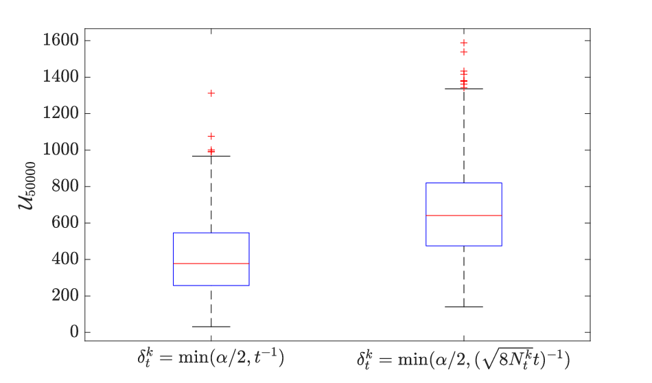
Additionally, Figure 8 presents boxplots of the regret and net safety at for the two schedules. An interesting observation is that the schedule exhibits greater variability, with some (rare) but massive outliers that are not present for the theoretical schedule. Investigating this more closely requires determining high-probability bounds on these methods, which is a subject for future work.

F.4 The behaviour of a Naïve Thompson Sampling Based Safety Index
As discussed in §4.2, a naïve way of constructing a safety index by just sampling should be ineffective when the safety score is close to We first investigate this effect.
Concretely, the scheme is the same as Alg.3, except that instead of the BayesUCB index, we construct a safety index by sampling as above, and then populate We run this scheme with the data
and vary as for . This corresponds to an increasing safety slack, while for the safety gap of the unsafe arm remains large, but decaying. Note that this ostensibly should increase the large regret for a scheme with optimal dependence.
Figure 9 plots the resulting mean regrets over a horizon of length 10K for four of the 10 cases (chosen evenly to not clutter the plot too much). The data is averaged over 200 trials. Observe that for wherein the gap is , the regret grows linearly, while the dependence becomes sublinear as increases, and further improves, even though it should grow like .


Further, we observe that the dependence on scales roughly as inverse-quadratic. This is illustrated in Figure 10, which plots both the mean regret against , as well as the mean of against . The key observation is the nearly linear dependence in the second plot for small . This observation makes sense - the variance scale of a distribution is as and so if the means is close to the truth, then the chance of falling above at time is roughly , and so for about rounds. Of course, for large enough this term is dominated by the regret terms due to suboptimal arms, and the dependence is masked. This effect is further confounded in our simulation with the fact that the safety gap reduces as is increased, which raises the regret. Nevertheless, the trend is evident, at least in the low regime where the gap does not change as much, and remains much larger than .


Despite the ineffectiveness when is small, a TS based safety index is an attractive proposition, primarily due to wider concerns - the advantage of TS for standard bandits is obtaining strong regret performance at a low computational cost, and this is specially important in cases such as combinatorial or continuously armed bandits. An alternative sampling based strategy would enable such an approach for safe bandits in such rich scenarios, and is of both practical and theoretical interest. Promisingly, when the gap is large, the effect on regret is indeed mild, showing that this is the only obstacle in the path of such a strategy.
One natural approach to address this obstacle is to allow a slack in the safety criterion for TS - we may sample according to the safety posterior, and then instantiate where serves as a slack. This raises a design question of how to choose this slack. We empirically investigate the choice of slack where is the standard deviation of the safety posterior or arm at time . This choice is natural, since this variance determines the scale of fluctuations of the score itself. Figure 11 shows the behaviour obtained as we set for for the same data as before, but now with fixed
This plot, while very preliminary, shows an interesting effect in that values of again result in large, linear regret. Recall that which corresponds to no slack, also gives linear regret. It is unclear how robust this effect is, but if true, this observation suggests that tuning this properly is a subtle problem, and the behaviour is quite sensitive to it, which raises an interesting challenge for further work.

