Assisted Shortest Path Planning for a Convoy through a Repairable Network
Abstract
In this article, we consider a multi-agent path planning problem in a partially impeded environment. The impeded environment is represented by a graph with select road segments (edges) in disrepair impeding vehicular movement in the road network. A convoy wishes to travel from a starting location to a destination while minimizing some accumulated cost. The convoy may traverse an impeded edge for an additional cost (associated with repairing the edge) than if it were unimpeded. A second vehicle, referred to as a service vehicle, is simultaneously deployed with the convoy. The service vehicle assists the convoy by repairing an edge, reducing the cost for the convoy to traverse that edge. The convoy is permitted to wait at any vertex to allow the service vehicle to complete repairing an edge. The service vehicle is permitted to terminate its path at any vertex. The goal is then to find a pair of paths so the convoy reaches its destination while minimizing the total time (cost) the two vehicles are active, including any time the convoy waits. We refer to this problem as the Assisted Shortest Path Problem (ASPP). We present a generalized permanent labeling algorithm to find an optimal solution for the ASPP. We also introduce additional modifications to the labeling algorithm to significantly improve the computation time and refer to the modified labeling algorithm as . Computational results are presented to illustrate the effectiveness of in solving the ASPP. We then give concluding remarks and briefly discuss potential variants of the ASPP for future work.
I INTRODUCTION
There has been an increasing interest in the study of cooperative behavior between multiple autonomous agents operating in a shared environment to complete some given task [1, 2, 3, 4, 5, 6]. This growing interest is due to the many applications which can make use of the cooperation of multiple agents, such as search-and-rescue [7], cooperative manipulation [8], foraging [9], surveillance[10], and safe escort using coordinated UAV and UGV systems [7, 11, 12, 13]. The manner in which the agents cooperate will vary depending on the collective goal considered. The agents may employ a divide-and-conquer approach and complete independent tasks, such as in a search-and-rescue application. The agents may instead be required to directly assist each other, such as in the case of cooperative manipulation where two or more agents work together to physically move an object in space (box-pushing [14]). A combination of these two approaches may also be considered, as in this paper. The use of multiple agents to complete a given task can potentially lead to performance improvements (faster times, more tasks done per unit cost, etc.). The use of multiple agents also allows for a wider variety of situations to be addressed. We refer the reader to [15] for a comprehensive survey of cooperative behavior of multiple autonomous agents.
The focus of this paper is the path planning of two autonomous agents operating in a partially impeded environment. As an example, this impeded environment may be a warehouse in which agents are organizing goods. The pathways in the warehouse may have some obstructions, such as fallen goods, that hinder the agents’ ability to maneuver. This impeded environment is represented by a graph where select edges represent obstructions using edge weights that will be defined later. These edges are assumed to be known a priori and are referred to as impeded edges. In the general case, obstructions may be physical or abstract. A designated agent, referred to as the convoy vehicle for the remainder of this paper, must leave a specified starting location and reach a given destination while minimizing some accumulated cost. The convoy will be assumed to have the capability to handle the obstructions present, but doing so will incur some cost in addition to the cost of travel. A second designated agent, referred to as the service vehicle for the remainder of this paper, can be simultaneously deployed to assist the convoy by clearing these obstructions itself as the convoy is traveling in the environment. As the service vehicle travels, it also incurs some cost. When the service vehicle clears an obstruction, it incurs some additional cost. Once an obstruction is cleared, it is assumed to remain cleared. The convoy may choose to wait at a vertex for some additional cost to allow the service vehicle to clear obstructions. The service vehicle may terminate at any vertex in the graph without continuing to incur additional cost as the convoy continues to its destination. The objective is then to find a pair of paths for the convoy and service vehicle such that the total cost accumulated for the two vehicles is minimized. For ease of discussion, we will refer to this problem as the Assisted Shortest Path Problem (ASPP). We provide a mathematical formulation for the ASPP in Section II.
Restricted variations of the ASPP have been studied in [16] and [17]. In these papers, the convoy was not able to clear any obstructions by itself. This is the same as the cost of the convoy traversing any impeded edge being infinite. In [16], a mixed-integer linear programming formulation was presented. An approximation algorithm was presented in [17] for the case where the convoy may share an impeded edge with the service vehicle. The addition of the convoy’s ability to traverse through impeded edges in this paper adds a significant level of complexity and allows for modeling more complex scenarios.
The main contribution of the paper is the development of a generalized, permanent labeling algorithm () that finds an optimal solution for the ASPP. Permanent labeling algorithms were introduced in [18] for the path planning of a single vehicle in a graph while adhering to various path structural constraints. In this approach [19], the state of the vehicle is stored as a label, and the label is updated as the vehicle moves to reflect the changes in the state. The key part of this approach lies in defining suitable labels and their updates so that partial solutions that can potentially lead to an optimal solution are not discarded. In this paper, we develop this approach to handle multiple, cooperative vehicles and solve the ASPP. After we develop the , we introduce filters to further reduce the search space and improve the performance of the algorithm. We refer to this refined with filters as . The procedure we present can be further generalized to handle more vehicles as needed.
The structure of this paper is as follows. Section II presents the mathematical formulation for the ASPP. Section III presents the and . Section IV presents computational results for and the . is shown to be significantly better than the . Several families of problem instances are constructed to show the influence of various aspects of the ASPP on the runtime of and the structure of optimal solutions to the ASPP. Section V presents concluding remarks and future work.
II Problem Statement
Let be an undirected, connected graph representing an impeded environment. is the set of vertices and is the set of undirected edges. The convoy and service vehicle start at vertices and , respectively, where and need not be distinct. Let be the destination of the convoy. The service vehicle may terminate at any vertex at any time and therefore has no destination. For the remainder of this paper, we will use cost and time interchangeably. Changes can be easily made to consider more general costs. Edges needing repair are known a priori and are referred to as impeded edges. The remaining edges are called unimpeded edges. We say an impeded edge is serviced if either the convoy or service vehicle has completely traversed that edge. In this paper, we use repair and service for an impeded edge interchangeably to indicate removing an obstruction (physical or abstract) in the impeded environment. We use the term impeded travel cost to refer to the cost for a vehicle to take an impeded edge that has not yet been serviced and use the term unimpeded travel cost otherwise. Each edge has four edge weights of the form . and are the unimpeded and impeded travel cost for the convoy, respectively. The unimpeded and impeded travel costs for the service vehicle are and , respectively. All costs are non-negative and are known. For unimpeded edges, and . For impeded edges, we have and . Therefore, the cost of the convoy taking edge is reduced if it is first serviced by the service vehicle. All edges are undirected so the cost in both directions are taken to be identical. When an impeded edge is serviced, it remains serviced.
We assume the following: (1) the convoy and service vehicles can share vertices and edges without conflict, (2) the two vehicles start at the same time, (3) the two vehicles communicate at all times and information is shared in a negligible amount of time, and (4) the service vehicle always travels faster than the convoy at any edge. The convoy is allowed to wait at any vertex to give the service vehicle time to repair impeded edges. Waiting will incur some additional cost. In this paper, this waiting cost is simply the time the convoy waits. We also allow the service vehicle to wait, but doing so will incur zero additional cost. This was done for two main reasons. First, depending on the application the service vehicle may be able to temporarily shut off or idle for a negligible amount of power consumption. Second, since the service vehicle is assumed to travel faster than the convoy and all costs are non-negative, it is clear an optimal solution will never have the service vehicle wait at a vertex and so we can set the wait cost to be zero for mathematical convenience. A more general waiting cost can be included, but the subsequent definitions and algorithms will need to be modified.
Let be a path from to for the convoy and be a path from to for the service vehicle. We note that a vehicle’s path will also potentially have waiting at one or more vertices. The two paths are coupled using the rules previously outlined. The cost of will depend on the decisions made by the service vehicle in path and vice-versa. We note that the service vehicle may also choose to remain at . The accumulated cost of these two paths is the sum of the time the convoy reaches and the time the service vehicle first reaches (it may choose to terminate at ) while adhering to the motion rules and travel cost rules. This cost includes any waiting time by the convoy. In other words, the accumulated cost is the total cost of the vehicles being active. If the service vehicle never initially leaves , the cost of is zero. We denote the total cost by ). The ASPP is then to find two coupled paths and , where is any vertex in , that minimizes .
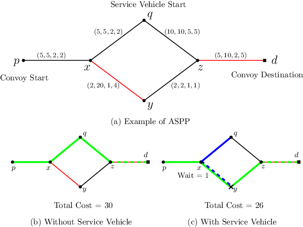
A sample problem for the ASPP is shown in Fig. 1(a). Fig. 1(b) represents the least-cost path for the convoy, with total cost , without the help of the service vehicle. The convoy will repair the edge in this solution. Fig. 1(c) represents the optimal solution with the help of the service vehicle. The service vehicle will take the path , repair the edge and then terminate at . The convoy will start from and wait at for unit of time to let the service vehicle finish the repair and traverse the serviced edge . The convoy will then repair the edge to reach the destination. The total cost for this solution is .
III Generalized Permanent Labeling Algorithms
We first define an abstract object called a label to store relevant information on decisions made by both vehicles. Recall the definition of a path and the accumulated cost from Section II.
Definition 1 (Label).
Suppose the convoy and service vehicle have taken paths and to and in in times and , including waiting, while accumulating a total cost . For each edge serviced by either vehicle, create a tuple where is the time edge was serviced. The set is the collection of the tuples . We then define a label as
For a label , we define to be the set of serviced edges in .
We next introduce resource extension functions (REFs) associated with each label. REFs describe how a label is extended to create a new label . Extending a label corresponds to feasible extensions of the paths and from decisions involving edges and , respectively. We allow for or , but not simultaneously11 1 Both and is not allowed because this condition implies both the vehicles are just waiting without performing any motion or servicing task. This clearly does not lead to an optimal solution..
Definition 2 (Resource Extension Functions).
Suppose paths and associated with label are extended by edges and , respectively, to create a new label . Let be the set of remaining impeded edges. Then,
The REFs in Definition 2 encode the cost rules previously outlined in Section II and tracks the edges that have been serviced and the times they were serviced. Each label is associated with a feasible trajectory pair, including the optimal solution. There are an infinite number of possible labels due to cycles and waiting. We introduce a dominance rule to reduce the number of labels under consideration to a finite number.
Definition 3 (Dominance Rule).
Consider two labels and . We say dominates if and only if
- 1.
- 2.
- 3.
- 4.
If , one label can be discarded arbitrarily if only one optimal solution is required. If all optimal solutions are needed, then keep both labels.
Conditions 1 and 2 state that both vehicles have reached the same pair of vertices in less time. Note that we do not require a separate dominance condition for cost as it follows from Conditions 1 and 2. If a more general cost is used, an additional condition must be included. Condition 3 states at least all serviced edges in have also been serviced in . Condition 4 states each serviced edge in was serviced earlier or at the same time in .
Theorem 1.
The extensions of only the non-dominated labels need to be considered to obtain the optimal solution.
Proof.
Let and be two distinct labels with dominating . We need to show any feasible extension of will be dominated by the same extension of .
Both and must have the same feasible extensions. Let the labels be extended by and for the convoy and service vehicle, respectively, resulting in new labels and . We allow for and , but not simultaneously. Using Definitions 2 and 3, we observe the following:
- •
If and , then we have .
- •
Suppose and . From ,
which implies .
- •
Suppose and . Then
which implies .
- •
Suppose . Since and , from Definition 2 we must have .
- •
Suppose and . Then
which implies .
- •
Suppose and . Then
which implies .
- •
The same extension is used so clearly implies .
- •
Suppose .
- –
If , from it follows that .
- –
If , then and so .
- –
- •
Suppose .
- –
If , from it follows that .
- –
If , then and so .
- –
We see will always dominate . Since the optimal solution must be a non-dominated label, we need to only consider non-dominated labels.
∎
From Theorem 1, we can solve the ASPP by repeatedly extending non-dominated labels, including the label corresponding to the initial configuration, until there are no more unique non-dominated labels that can be generated. Then, the non-dominated label that has the convoy position at and with the lowest cost corresponds to an optimal solution.
We also make a few trivial observations for optimal solutions to the ASPP that will reduce the number of non-dominated labels to consider:
- (i)
The service vehicle will never begin to move again after pausing at a vertex.
- (ii)
The service vehicle, if deployed, will only terminate immediately after servicing all of its assigned impeded edges.
- (iii)
The convoy will only wait at an end of an impeded edge it uses later.
- (iv)
A convoy waiting to use an impeded edge will wait until the service vehicle has serviced that edge.
- (v)
The convoy will never wait at a vertex after the service vehicle has terminated its motion.
These observations are a direct consequence of the structure of the cost rules from Section II. It should be noted these observations may not hold for more general cost structures and variants of the ASPP involving additional constraints. Using these observations, we can filter some extensions of non-dominated labels that will never eventually result in an optimal solution. To do this, we introduce two Boolean variables and for each label and write
is true when the service vehicle has terminated and is false otherwise. The label associated with the initial state of the vehicles has set to false by default. When extending a label with currently set to false, we create (1) all feasible extensions where and set to false and (2) all feasible extensions with set to true. From observation (i), we can enforce remain true for all extensions of a label with set to true. The variable is initially set to false and is defined in the following manner: Consider a label where the convoy is at vertex that is an end of an impeded edge . For this impeded edge, the extension of will create (1) a label with set to true and (2) a label with set to false. Next, consider a label with set to true. When extending , we create (1) all labels where and (2) all labels with set to true. When extending a label results in the convoy moving to a new vertex, is set to false. From this definition, captures the cooperative behavior between the service vehicle and the convoy when interacting with impeded edges. The rules for updating and can be directly included with the REFs in Definition 2.
The generalized permanent labeling algorithm () then works as follows. We create an initial label , false, false). We initialize two lists and with . We then take out of to find all its feasible extensions using the REFs of Definition 2 and the additional extension rules for and previously described. The non-dominated extensions are then added to and . We continue the process of using a chosen selection rule (last-in-first-out or LIFO in our implementation) to remove a label from , find its extensions, and store the resulting non-dominated labels in and . If a label with is removed from , we do not extend it. This processes is repeated until no longer has any labels to extend and the algorithm terminates. Once the algorithm has terminated, the label in with minimum cost corresponds to an optimal solution to the ASPP. The trajectories for the optimal solution can be found by iteratively going through the predecessors of the label. Therefore, we require some way to store the predecessor label for any given label . We have done this by directly including the parent label in the definition of in our implementation.
III-A Generalized Permanent Labeling Algorithm - ()
We now introduce two final modifications to the permanent labeling algorithm to further reduce the number of labels that need to be extended and the overall computation time as a result. These modifications are motivated by the algorithm [20] used for solving the single agent shortest path planning problem. Therefore, we refer to with these modifications as . Algorithm 1 shows the pseudo-code for .
III-A1 Early Termination
In , we repeatedly extend labels from until we have exhausted all possible non-dominated labels. In general, the selection rule used to choose labels from to be extended can be arbitrary. The algorithm will always converge to the optimal solution irrespective of any selection rule. In permanent labeling algorithms, it is common to select the label most recently added to (LIFO) or find the label in with the least cost (best-first). The selection rule used can have a significant impact on the termination time of the algorithm.
For a single agent shortest path planning problem, the algorithm uses a heuristic-cost-based extension method to reach the destination while reducing the search space. We use a similar approach. For any label , we define the heuristic cost to be a lower bound on the cost for the convoy to reach from . In our implementation, we have taken to be the least cost path from to while treating all impeded edges as unimpeded, i.e., we set the edge weight to be for each edge. We define -cost for to be the sum of and . In other words, -cost is a lower bound on the cost for the convoy to reach the destination from the state corresponding to .
Lemma 1.
If a label with the least -cost is selected to be extended at every iteration, then the first such label with will correspond to an optimal solution to the ASPP.
Proof.
From Definition 2, for any extension from to , we have . We then see
which implies that the -cost will never decrease with extensions. Let be the first label with the convoy at the destination selected to be extended. This implies that all the other labels will have -cost greater than or equal to the -cost of . Note that -cost of is equal to . This implies that no other label can reach the destination with total cost lower than . ∎
In order to utilize the result in Lemma 1, we sort by the -cost of each label and use a best-first selection rule to select the label with the smallest -cost (Line 6 of Algorithm 1). When a label with is selected, the algorithm terminates and this label is returned as the optimal solution. The heuristic cost at each vertex is computed before starting the algorithm. This is indicated by the input in Algorithm 1.
III-A2 Cost filter
As previously discussed, when extending a label we only keep the resulting non-dominated labels. Checking for dominance is computationally expensive due to the third and fourth conditions of Definition 3. To further reduce the number of dominance checks needed, we compute an upper bound on the optimal solution to the ASPP before starting the labeling algorithm and use this upper bound to prematurely discard non-dominated labels. The upper bound used is the shortest path for the convoy from to without deploying the service vehicle. In other words, we set the cost of each unimpeded edge to be and the cost of each impeded edge to be and find the shortest path on with these edge weights. When a label is generated, before checking for dominance we check if the -cost exceeds the upper bound and if so we discard the label.
IV Results
All algorithms were implemented in Python 3.6 and the computations were done on an MSI laptop (8 Core Intel i7-7700HQ processor @ 2.80 GHz, 16 GB RAM). For the analysis, we used a grid structure for the graph as it can easily represent a real-world scenario, like a warehouse, and is also easy to reproduce for verification. For all of the instances, the origin and the destination of the convoy, and , were chosen to be at diagonally opposite ends of the grid to avoid trivial cases. Impeded edges can be chosen randomly or strategically so that the convoy has to traverse through at least one impeded edge to reach the destination. This can be achieved by choosing the impeded edges to make a cut between and . A cut between and for an instance is defined as the set of edges for any two disjoints sets , such that and and . An instance with cuts is constructed so that the impeded edge set only consists of edges from randomly chosen cuts.
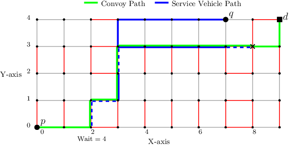
To help illustrate the graph structure used in the subsequent computational studies, Fig. 2 provides a sample instance. In Fig. 2, the convoy and service vehicle optimal solution paths are presented on the graph. In this instance, we have set and for all edges and set and for all impeded edges. In the optimal solution, the service vehicle starts from and repairs the following sequence of impeded edges: , , and . The convoy has to wait at for units of time in the optimal solution. The optimal solution cost for this instance is .
The remainder of this section is as follows. We first show a comparison between the run times of and . Next, we analyze over three different classes of instances. In Class 1, we aim to test the computational limits of as we increase the graph size and the number of impeded edges. In Class 2, we want to study the significance of unavoidable impeded edges on the optimal solution cost. We accomplish this by increasing the number of cuts on a grid graph of fixed size. Finally, Class 3 instances are designed to understand the impact of the service vehicle starting position on the optimal solution.
IV-A Comparison between and
To compare and , we have created grid instances with randomly chosen impeded edges while enforcing the fraction of impeded edges to be for every instance. The grid sizes were varied with increasing size and can be seen in Table I. For each grid size, 50 instances were generated. The starting position of the service vehicle was chosen randomly for each instance. For the convoy, the unimpeded travel cost, , was randomly chosen from the range for all edges and the impeded travel cost, , was randomly chosen from the range for the impeded edges. For the service vehicle, the unimpeded travel cost, , was set to be unit for all edges and the impeded travel cost, , was randomly chosen from the range for the impeded edges. For unimpeded edges, and . This cost structure was chosen to encourage collaboration between the vehicles while keeping the decision-making non-trivial.
| Grid-Size | ||||
|---|---|---|---|---|
| 25 ms | 0.6 ms | 578 | 10 | |
| 1.1 s | 0.6 ms | 8180 | 14 | |
| 149 s | 0.7 ms | 111804 | 17 | |
| 283 s | 0.9 ms | 189365 | 28 |
| = 0.3 | = 0.4 | = 0.5 | ||||
|---|---|---|---|---|---|---|
| Grid Size | time (sec.)* | time (sec.)* | time (sec.)* | |||
| 66 | 0.47 2.5 | 1.00 | 7.6 27 | 1.00 | 99 201 | 0.86 |
| 77 | 14 67 | 1.00 | 58 162 | 0.88 | 197 303 | 0.48 |
| 88 | 17 66 | 0.96 | 105 205 | 0.70 | 145 210 | 0.22 |
| 99 | 43 144 | 0.86 | 148 250 | 0.48 | 158 189 | 0.12 |
| 1010 | 45 119 | 0.80 | 126 223 | 0.36 | 128 129 | 0.08 |
time indicates the average computation time standard deviation.
Table I shows the comparison between the two algorithms and highlights the effectiveness of over . Both algorithms always result in the same optimal solution cost, hence it is not included in Table I. Each row represents the average value over randomly generated instances. and represents the average computational time for and , respectively. and shows the average number of extended labels for both algorithms. The comparison between the computation times and the extended labels clearly indicate the effectiveness of the modifications introduced for .
IV-B Class 1 instances
To test the computational limits of the , we generated instances from to grid sizes. For each instance, the impeded edges were chosen randomly and we used the same cost structure as in IV-A. The fraction of impeded edges is denoted by . For each grid size, the fraction of impeded edges were varied to be 0.1, 0.2, 0.3, 0.4, and 0.5. We generated random instances for each grid size and fraction of impeded edges. The starting position for the service vehicle was chosen randomly for each instance. An instance is said to be successful if it terminated with the optimal solution within 900 seconds. The success rate () is defined as the fraction of all successful instances over the total number of instances. For a majority of the instances with and , we observed that the impeded edges did not form a cut and so the convoy had at least one unimpeded path from to . Therefore, we do not include those results in our discussion.
The results for Class 1 are shown in Table II. In Table II, each entry in the time columns represents the average computation time of successful instances along with the standard deviation. We see the success rate decreases with increasing grid size and increasing fraction of impeded edges. The average computation time and the standard deviation increase with increase in grid size and fraction of impeded edges. For cases with relatively low success rate (), the average computation time may not follow the same trend as the samples are skewed. From this set of instances, we see the computation time is significantly affected by the number of impeded edges. This is to be expected, as must produce additional labels whenever a label is such that the convoy position is an end of an impeded edge. Similarly, an additional label is also generated whenever an extension is such that the service vehicle traverses an impeded edge, servicing it. As the number of impeded edges increases, the number of additional labels generated will begin to explode. The upper bound cost filter introduced for significantly reduces the number of redundant labels generated. However, as the graph size also increases the upper bound becomes less tight and so the algorithm begins to fail to discard redundant labels early. This behavior can be seen by noticing as the fraction of impeded edges increases for a fixed grid size, the computation time begins to grow at an exponential rate. Conversely, for a fixed fraction of impeded edges, the computation time grows more slowly as the grid size increases.
IV-C Class 2 instances
For this set of instances, we wish to determine how the presence of unavoidable impeded edges affects the optimal solution cost. To do this, we use a fixed grid of size with the same cost structure defined in IV-A for each instance. We then generated cuts to introduce unavoidable impeded edges for the convoy. The narrow grid structure was chosen as it is easier to produce cuts with fewer edges, which keeps the computational time reasonable as we increase the number of cuts. The service vehicle’s starting position was chosen randomly for each instance. The number of cuts was varied form 1 to 5. We generated 50 random instances for each cut size.
| Cuts | |||||
|---|---|---|---|---|---|
| 1 | 0.05 | 191 | 0.89 | 1.05 | 6.19 |
| 2 | 0.10 | 196 | 0.82 | 1.08 | 6.48 |
| 3 | 0.14 | 201 | 0.77 | 1.10 | 6.94 |
| 4 | 0.18 | 205 | 0.71 | 1.12 | 6.90 |
| 5 | 0.22 | 207 | 0.68 | 1.14 | 7.56 |
The computational results for this set of instances is shown in Table III. Each row in Table III represents an average value over the instances for a set number of cuts. Column indicates the fraction of impeded edges. An upper bound, , was computed by having the convoy take the shortest path from to without any assistance from the service vehicle. The gap between the cost of the optimal solution to the ASPP and gives an indicator of the benefit of deploying the service vehicle.
Similarly, a lower bound, , was computed by treating all impeded edges as unimpeded and finding the shortest path for the convoy from to only using the unimpeded cost for all edges.
Columns and represents the ratio of optimal cost, , against the upper bound and the lower bound costs, respectively.
We see as the number of cuts increases, the ratio decreases.
This shows the effectiveness/benefit of the service vehicle in an impeded environment, especially as the number of unavoidable impeded edges increases.
Column shows the standard deviation of the optimal cost. The increasing trend of indicates that the optimal solution cost is sensitive to the number of unavoidable impeded edges.
IV-D Class 3 instances
For this set of instances, we examine the impact of the starting position of the service vehicle on the optimal solution. For each instance, we again use a grid, but we impose a fixed cost structure for all instances. All edges were assigned costs and and the impeded edges were all assigned costs and . The convoy’s starting position and destination were fixed at diagonally opposite ends with positions and (see Figure 3). This cost structure and choice of positions were chosen to encourage collaboration between the convoy and service vehicle. We generated 50 different instances by randomly generating 3 cuts for each instance. For a given instance, we compute the optimal solution cost for each of the 45 possible starting positions for the service vehicle. We then computed the average optimal cost across all 50 instances for each of the 45 service vehicle starting positions.

Fig. 3 shows the average cost across instances for each starting position in the grid. The convoy starting position and destination are marked at and . Gaussian interpolation was used to generate a continues map. We observe that the minimum and maximum average costs are achieved at vertex and respectively. Fig. 3 shows the starting position of the service vehicle will have a noticeable impact on the optimal solution. The magnitude of the impact will depend on the numerical values of the costs for the edges. We also note the best starting position for the service vehicle in this set of instances does not coincide with the starting position of the convoy. This is to be expected. If the service vehicle starts some distance away from the convoy, it may be able to attend to more significant impeded edges before the convoy is able to reach them.
V Conclusion and Future Work
In this article, we considered an assisted path planning problem for a convoy and a service vehicle in an impeded environment. Although the convoy is capable of traversing impeded edges, the service vehicle can help the convoy to reach the destination with a lower total accumulated cost. A generalized permanent labeling algorithm () was presented to solve the ASPP to optimality. Additional modifications were introduced to reduce the search space and the overall computational time as a result. The modified algorithm is referred as . Computational results showed the effectiveness of the modifications in when compared to . Another computational study was done to show the computational performance of as the problem size increased and as the number of impeded edges increased. It was found the number of impeded edges has a more significant impact on the computation time of versus the overall size of the problem (i.e., the number of vertices). Two more computational studies were performed to study the impact of the presence of the number of unavoidable impeded edges and of the starting position of the service vehicle on the optimal solution to the ASPP.
The future potential extensions of this problem may include limited communication range between the vehicles or the use of specialized service vehicles that can only repair some specific type of impeded edge. A non-deterministic version of ASPP can also be considered where a probability density function is assigned with the travel cost of an impeded edge.
References
- [1] G. Wagner and H. Choset, “Subdimensional expansion for multirobot path planning,” Artificial intelligence, vol. 219, pp. 1–24, 2015.
- [2] G. Sharon, R. Stern, A. Felner, and N. R. Sturtevant, “Conflict-based search for optimal multi-agent pathfinding,” Artificial Intelligence, vol. 219, pp. 40–66, 2015.
- [3] B. De Wilde, A. W. Ter Mors, and C. Witteveen, “Push and rotate: cooperative multi-agent path planning,” in Proceedings of the 2013 international conference on Autonomous agents and multi-agent systems, pp. 87–94, 2013.
- [4] T. Standley, “Finding optimal solutions to cooperative pathfinding problems,” in Proceedings of the AAAI Conference on Artificial Intelligence, vol. 24, pp. 173–178, 2010.
- [5] M. Erdmann and T. Lozano-Perez, “On multiple moving objects,” Algorithmica, vol. 2, no. 1, pp. 477–521, 1987.
- [6] D. Silver, “Cooperative pathfinding,” in Proceedings of the aaai conference on artificial intelligence and interactive digital entertainment, vol. 1, pp. 117–122, 2005.
- [7] J. Li, G. Deng, C. Luo, Q. Lin, Q. Yan, and Z. Ming, “A hybrid path planning method in unmanned air/ground vehicle (uav/ugv) cooperative systems,” IEEE Transactions on Vehicular Technology, vol. 65, no. 12, pp. 9585–9596, 2016.
- [8] L. Parker, Heterogeneous multi-robot cooperation. PhD thesis, MIT, 1994.
- [9] L. Steels, “Cooperation between distributed agents through self-organization,” IEEE International Workshop on Intelligent Robots and Systems, Towards a New Frontier of Applications, pp. 8–14, 1990.
- [10] L. E. Parker, “Cooperative robotics for multi-target observation,” Intelligent Automation & Soft Computing, vol. 5, no. 1, pp. 5–19, 1999.
- [11] S. Minaeian, J. Liu, and Y.-J. Son, “Vision-based target detection and localization via a team of cooperative uav and ugvs,” IEEE Transactions on systems, man, and cybernetics: systems, vol. 46, no. 7, pp. 1005–1016, 2015.
- [12] E. Garcia and D. Casbeer, “Coordinated threat assignments and mission management of unmanned aerial vehicles,” Cooperative Control of Multi-Agent Systems: Theory and Applications, p. 141, 2017.
- [13] T. H. Chung, “Offensive swarm-enabled tactics (offset),” DARPA, 2021.
- [14] B. Donald, J. Jennings, and D. Rus, “Analyzing teams of cooperating mobile robots,” Proceedings of the 1994 IEEE International Conference on Robotics and Automation, vol. 3, pp. 1896–1903, 1994.
- [15] Y. Cao, A. Fukunaga, and A. Kahng, “Cooperative mobile robotics: Antecedents and directions,” Autonomous Robots, pp. 7–27, 1997.
- [16] C. Montez, S. Rathinam, S. Darbha, and D. Casbeer, “Finding shortest paths for a team of convoy and repair vehicles,” in AIAA Scitech 2021 Forum, p. 1769, 2021.
- [17] C. Montez, S. Rathinam, S. Darbha, D. Casbeer, and S. G. Manyam, “An approximation algorithm for an assisted shortest path problem,” in 2021 IEEE International Conference on Robotics and Automation (ICRA), pp. 8024–8030, IEEE, 2021.
- [18] M. Desrochers and F. Soumis, “A generalized permanent labelling algorithm for the shortest path problem with time windows,” INFOR: Information Systems and Operational Research, vol. 26, no. 3, pp. 191–212, 1988.
- [19] S. Irnich and G. Desaulniers, “Shortest path problems with resource constraints,” in Column generation, pp. 33–65, Springer, 2005.
- [20] P. E. Hart, N. J. Nilsson, and B. Raphael, “A formal basis for the heuristic determination of minimum cost paths,” IEEE transactions on Systems Science and Cybernetics, vol. 4, no. 2, pp. 100–107, 1968.