Dipole-dipole Interactions Through a Lens

Technological advances in the last decade have facilitated the probing and control of single atoms by collecting and focusing light with the help of high numerical aperture (NA) lenses. Some example of this progress are quantum gas microscopes Bakr et al. 2009; Cheuk et al. 2015; Parsons et al. 2015; Haller et al. 2015; Yamamoto et al. 2016, programmable atom arrays Endres et al. 2016; Barredo et al. 2016; Kaufman and Ni 2021, and other novel arrangements of lenses to improve atom-field interfaces Chin et al. 2017; Bianchet et al. 2021. State-of-the-art optical elements allow for an NA as high as 0.92 Robens et al. 2017, near the theoretical limit. The rapid progress of such tools opens new possibilities to enhance and manipulate long-range atom-atom interactions.

The ability to collect light from an emitter and guide it over long distances enables a variety of collective quantum optical phenomena, which has been a subject of significant interest in recent theoretical Asenjo-Garcia et al. 2017; Sinha et al. 2020a; Sinha et al. 2019; Dinc and Braǹczyk 2019; Calajó et al. 2019; Sheremet et al. 2021; Trivedi et al. 2021; Buonaiuto et al. 2021; Poshakinskiy and Poddubny 2021; Pivovarov et al. 2021; Jones et al. 2020; Arranz Regidor et al. 2021 and experimental works van Loo et al. 2013; Solano et al. 2017; Kim et al. 2018; Newman et al. 2018; Boddeti et al. 2022 in waveguide quantum electrodynamics (QED). Typically, these implementations rely on the evanescent light-matter coupling wherein the emitters are either placed nearby or embedded in a solid waveguide structure. This introduces various dissipation and decoherence mechanisms and hinders the control and probing of both the atoms and the electromagnetic (EM) field Fermani et al. 2007; Yeung and Gustafson 1996; Scheel et al. 2005; Rekdal et al. 2004; Skagerstam et al. 2006; Sagué et al. 2007. On the contrary, imaging systems involve large distances of operation that allow one to treat the atoms as if they were in free space, while facilitating interactions with their distant counterparts.

At a fundamental level in QED, the interactions between two atoms are mediated by the quantum fluctuations of the EM field. Such interactions depend on the range of separation between the two atoms Goldstein and Meystre 1997; Milonni and Knight 1974; Sinha et al. 2020b, boundary conditions on the EM field Dung et al. 2002; Kobayashi et al. 1995; Goldstein et al. 1996; El-Ganainy and John 2013; Agarwal and Gupta 1998; Hopmeier et al. 1999; Haugland et al. 2021 and its spectral density John and Quang 1995; Bay et al. 1997a; Bay et al. 1997b; Xie et al. 2003; Kurizki 1990; Cortes and Jacob 2017, quantum correlations between the atoms Behunin and Hu 2010; Jones et al. 2018; Sinha et al. 2018; Yang et al. 2020, external classical driving fields Yang et al. 2020; Varada and Agarwal 1992; de Léséleuc et al. 2017, among other factors. In this work we explore the idea of using an ideal lens together with a weak external drive to amplify and engineer the interaction between two distant atoms. As the atoms scatter the laser field, the lens collects and amplifies the far-field resonant dipole-dipole interaction mediated via the drive photons. This opens the possibility of using atomic imaging technology for engineering long-range dipole-dipole interactions and implementing collective systems without the downsides of near-field interactions.

The rest of the paper is organized as follows. In Sec. II we describe the system consisting of two two-level atoms placed near each focal point of an ideal, aberration free, aplanatic lens. We derive the collective atomic master equation in Sec. III and the Green’s tensor for the EM field propagation in Sec. IV. This allows one to obtain the dispersive and dissipative contributions to the effective dipole-dipole interaction in Sec. V. In Sec. VI, we analyze the effects of such lens-mediated enhancement of the far-field resonant dipole-dipole interaction and the possibility of creating a mutual trap potential for atoms interacting via lenses. We finalize presenting a brief outlook and concluding remarks in Sec. VII.

We consider a system of two two-level atoms (A1 and A2) separated by an aplanatic lens, as shown in Fig. 1. An aplanatic lens is generally composed of two or three lenses such that spherical and coma aberrations are suppressed Pedrotti et al. 2006. For the purposes of this work, we describe the lens in terms of its effects on the EM field wavefront, regardless of the details of the elements that it is comprised of. The atoms are placed near the focal points on each side of the lens. The system exhibits azimuthal symmetry, that can be broken by the polarization of the atomic dipoles deviating from the optical axis. We further assume that the atoms are weakly driven by a classical field of frequency $\omega_{D}$.

The total Hamiltonian of the system is given by $H=H_{A}+H_{F}+H_{AF}+H_{AD}$, where $H_{A}$ corresponds to the Hamiltonian for the two atoms in the rotating frame with respect to the drive frequency:

$\displaystyle H_{A}=$

$\displaystyle\hbar\delta_{D}\sum_{a}\hat{\sigma}_{+}^{(a)}\hat{\sigma}_{-}^{(a)}$

(1)

with $\hat{\sigma}_{+}^{(a)}\equiv\left|e_{a}\right\rangle\left\langle g_{a}\right|$ and $\hat{\sigma}_{-}^{(a)}\equiv\left|g_{a}\right\rangle\left\langle e_{a}\right|$ as the raising and lowering operators for the internal degrees of freedom of the atoms labeled by $a=1,2$ which corresponds to the atoms A1 and A2 respectively, and $\delta_{D}=\omega_{0}-\omega_{D}$ as the detuning between the atomic resonance $\omega_{0}$ and the drive frequency.

The atom-vacuum and atom-drive interaction Hamiltonians in the rotating frame are respectively given as:

	$\displaystyle H_{AF}=$	$\displaystyle-\sum_{a}\hat{{\mathbf{p}}}_{a}\cdot\hat{{\mathbf{E}}}\left({\mathbf{r}}_{a}\right),\text{and}$		(2)
	$\displaystyle H_{AD}=$	$\displaystyle\sum_{a}\hbar\Omega\left[\sigma_{+}^{(a)}+\sigma_{-}^{(a)}\right].$		(3)

The atomic dipole operator for each atom in the rotating frame is given by $\hat{\mathbf{p}}_{a}=\mathbf{d}_{a}^{\dagger}\hat{\sigma}_{+}^{(a)}e^{i\omega_{D}t}+\mathbf{d}_{a}\hat{\sigma}_{-}^{(a)}e^{-i\omega_{D}t}$, with $\mathbf{d}_{a}$ the dipole matrix element associated with the $\left|g_{a}\right\rangle\leftrightarrow\left|e_{a}\right\rangle$ transition. $\hat{{\mathbf{E}}}\left({\mathbf{r}}_{a}\right)$ represents the electric field at position ${\mathbf{r}}_{a}$ of atom $a$. The Rabi frequency of the drive is given by $\Omega$. We note that in the presence of a weak classical drive, the atomic dipoles exhibit Rayleigh scattering at the drive frequency.

The field Hamiltonian $H_{F}$ and the quantized EM field in the presence of media are described in the macroscopic QED formalism Gruner and Welsch 1996; Buhmann and Welsch 2007; Dung et al. 2002; Buhmann 2012a; Buhmann 2012b, as discussed in Appendix A.

We can now describe the dynamics of the atomic internal degrees of freedom in terms of a second-order Lindblad master equation by tracing out the EM field in the Born-Markov approximations (see Appendix B for details) Breuer and Petruccione 2002; Sinha et al. 2018:

$\displaystyle\frac{{d}\rho_{A}}{{d}t}=-\frac{i}{\hbar}\left[H_{A}^{\prime},\rho_{A}\right]+\mathcal{L}_{A}\left[\rho_{A}\right],$

(4)

where $\rho_{A}$ corresponds to the collective density matrix of the two atoms. The effective Hamiltonian $H_{A}^{\prime}$ and the Liouvillian $\mathcal{L}_{A}$ describe the dispersive and the dissipative dynamics of the collective atomic system in the presence of the aplanatic lens:

	$\displaystyle H_{A}^{\prime}=$	$\displaystyle\sum_{i,j=1,2}J^{(+)}_{ij}\hat{\sigma}_{+}^{(i)}\hat{\sigma}_{-}^{(j)}+J^{(-)}_{ij}\hat{\sigma}_{-}^{(i)}\hat{\sigma}_{+}^{(j)},$		(5)
	$\displaystyle\mathcal{L}_{A}\left[\rho_{A}\right]=$	$\displaystyle-\frac{1}{2}\sum_{i,j=1,2}\Gamma_{ij}\left\{\hat{\sigma}_{+}^{(i)}\hat{\sigma}_{-}^{(j)},\rho_{A}\right\}$
		$\displaystyle+\sum_{l}\int d^{3}\mathbf{k}\hat{\mathcal{O}}^{(i)}_{{\mathbf{k}}l}\rho_{A}\left(\hat{\mathcal{O}}^{(j)}_{{\mathbf{k}}l}\right)^{\dagger}.$		(6)

The coherent couplings between the two atoms and the individual energy modifications to the excited and ground states of the atoms are given by $J_{ij}^{(+)}=-J_{ij}^{\mathrm{OR}}-J_{ij}^{\mathrm{R}}$ and $J_{ij}^{(-)}=J_{ij}^{\mathrm{OR}}$. The off-resonant and the resonant contributions $J_{ij}^{\mathrm{OR}}$ and $J_{ij}^{\mathrm{R}}$ correspond to the contributions from virtual and real photons, respectively, and are given explicitly as follows:

	$\displaystyle J_{ij}^{\mathrm{OR}}$	$\displaystyle\equiv\frac{\mu_{0}\omega_{D}}{\pi}\int_{0}^{\infty}\mathrm{d}\xi\,\frac{\xi^{2}}{\xi^{2}+\omega_{D}^{2}}\left({\bf d}^{\dagger}\cdot{\stackrel{{\scriptstyle\leftrightarrow}}{{\mathbf{G}}}\left({\bf r}_{i},{\bf r}_{j},i\xi\right)}\cdot{\bf d}\right)$		(7)
	$\displaystyle J_{ij}^{\mathrm{R}}$	$\displaystyle\equiv\mu_{0}\omega_{D}^{2}\mathrm{Re}\left[{\bf d}^{\dagger}\cdot{\stackrel{{\scriptstyle\leftrightarrow}}{{\mathbf{G}}}\left({\bf r}_{i},{\bf r}_{j},\omega_{D}\right)}\cdot{\bf d}\right].$		(8)

We note that while the off-resonant part depends on the broadband frequency response of the environment, the resonant part only depends on the response of the EM environment at the drive frequency.

The dissipative interaction between the atoms is given by:

$\displaystyle\Gamma_{ij}\equiv$

$\displaystyle\frac{2\mu_{0}\omega_{D}^{2}}{\hbar}\,{{\bf d}^{\dagger}\cdot\mathrm{Im}\left[\stackrel{{\scriptstyle\leftrightarrow}}{{\mathbf{G}}}\left({\bf r}_{i},{\bf r}_{j},\omega_{D}\right)\right]\cdot{\bf d}},$

(9)

which is related to the resonant dispersive interaction $\left(J_{ij}^{\mathrm{R}}\right)$ via the Kramers-Kronig relation Buhmann 2012b.

The jump operator $\hat{\mathcal{O}}_{{\mathbf{k}},l}^{(i)}$ for atom $i$ Chang et al. 2014:

		$\displaystyle\mathcal{\hat{O}}_{{\mathbf{k}},l}^{(i)}=$
		$\displaystyle\sqrt{\frac{2\epsilon_{0}\mu_{0}^{2}\omega_{D}^{4}}{\hbar}}\int\mathrm{d}^{3}r\frac{e^{i{\mathbf{k}}\cdot{\mathbf{r}}}}{\left(2\pi\right)^{3/2}}\sqrt{\epsilon\left({\mathbf{r}},\omega_{D}\right)}{\mathbf{d}}_{i}{G}_{il}\left({\mathbf{r}}_{i},{\mathbf{r}},\omega_{D}\right)\hat{\sigma}^{(i)}_{-},$		(10)

corresponds to the process of recoil of a photon of frequency $\omega_{D}$, momentum $k$ and polarization $l$; similarly for atom $j$. It can be seen that $\sum_{l}\int\mathrm{d}^{3}{\mathbf{k}}\left(\hat{\mathcal{O}}^{(i)}\right)^{\dagger}_{{\mathbf{k}},l}\hat{\mathcal{O}}^{(j)}_{{\mathbf{k}},l}=\hbar\Gamma_{ij}\hat{\sigma}^{(i)}_{+}\hat{\sigma}^{(j)}_{-}$.

When analyzing the far-field contributions to the dipole-dipole interactions amplified by the lens we can neglect the off-resonant contributions from virtual photons at second-order $(J_{ij}^{\mathrm{OR}})$ that scale as $\sim 1/r^{3}$, and those at fourth-order that scale as $\sim 1/r^{6}$. The predominant contribution is the resonant dipole-dipole interaction given by Eq. (8), which scales as $\sim 1/r$, and depends only on the response of the environment at the drive frequency $\omega_{D}$.

We describe the electric field at a given point ${\mathbf{r}}$ emitted by a dipole at the position ${\mathbf{r}}_{0}$ in terms of the classical EM Green’s tensor Buhmann 2012a; Buhmann 2012b, defined by the inhomogeneous Helmholtz equation as follows:

$\displaystyle\left[\frac{1}{\mu_{0}}{\mathbf{\nabla}}\times{\mathbf{\nabla}}\times-\frac{\omega^{2}}{c^{2}}\epsilon\left({\mathbf{r},\omega}\right)\right]\stackrel{{\scriptstyle\leftrightarrow}}{{\mathbf{G}}}\left({\mathbf{r}},{\mathbf{r}}_{0},\omega\right)=\delta\left({\mathbf{r}}-{\mathbf{r}}_{0}\right),$

(11)

together with the condition that $\stackrel{{\scriptstyle\leftrightarrow}}{{\mathbf{G}}}\left({\mathbf{r}},{\mathbf{r}}_{0},\omega\right)\rightarrow 0$ as $\left|{\mathbf{r}}-{\mathbf{r}}_{0}\right|\rightarrow\infty$. One can separate the contributions to the field in terms of the distance between the the two points as:

	$\displaystyle\stackrel{{\scriptstyle\leftrightarrow}}{{\mathbf{G}}}\left({\mathbf{r}},{\mathbf{r}}_{0},\omega\right)=$	$\displaystyle\stackrel{{\scriptstyle\leftrightarrow}}{{\mathbf{G}}}_{\mathrm{NF}}\left({\mathbf{r}},{\mathbf{r}}_{0},\omega\right)+\stackrel{{\scriptstyle\leftrightarrow}}{{\mathbf{G}}}_{\mathrm{IF}}\left({\mathbf{r}},{\mathbf{r}}_{0},\omega\right)$
		$\displaystyle+\stackrel{{\scriptstyle\leftrightarrow}}{{\mathbf{G}}}_{\mathrm{FF}}\left({\mathbf{r}},{\mathbf{r}}_{0},\omega\right),$		(12)

where $\stackrel{{\scriptstyle\leftrightarrow}}{{\mathbf{G}}}_{\mathrm{NF}}\left({\mathbf{r}},{\mathbf{r}}_{0},\omega\right)$, $\stackrel{{\scriptstyle\leftrightarrow}}{{\mathbf{G}}}_{\mathrm{IF}}\left({\mathbf{r}},{\mathbf{r}}_{0},\omega\right)$ and $\stackrel{{\scriptstyle\leftrightarrow}}{{\mathbf{G}}}_{\mathrm{FF}}\left({\mathbf{r}},{\mathbf{r}}_{0},\omega\right)$ correspond to the near-field, intermediate-field and far-field contributions, respectively. Since the distance between the emitter and the lens is much greater than the wavelength of the emitted field, we will only be interested in the far-field contribution Buhmann 2012a; Buhmann 2012b; Novotny and Hecht 2012.

Let ${\mathbf{r}}_{1}$ and ${\mathbf{r}}_{2}$ be the positions of the atoms A1 and A2, as depicted in Fig. 2. The resonant electric field produced by an arbitrarily oriented electric dipole located at ${\mathbf{r}}_{1}$, with dipole moment $\mathbf{p}$, after propagation to a point $\mathbf{r}$ at the vacuum-lens interface is:

$$\mathbf{E}_{\mathrm{FF}}\left({\mathbf{r}},{\mathbf{r}}_{1}\right)=-\frac{\omega^{2}_{D}}{\varepsilon_{0}c^{2}}\stackrel{{\scriptstyle\leftrightarrow}}{{\mathbf{G}}}_{\mathrm{FF}}\left({\mathbf{r}},{\mathbf{r}}_{1},\omega_{D}\right)\cdot\mathbf{p}.$$

(13)

The field is collimated after transmission through the first interface of the aplanatic lens, travels as a collimated beam until it reaches the second interface on the opposite side after which it converges at the focal point on the other side. To obtain the field in the region near the second focus, we use the angular spectrum representation in cylindrical coordinates $\left\{\rho,\varphi,z\right\}$ Novotny and Hecht 2012:

	$\displaystyle\mathbf{E}_{\mathrm{fo}}(\rho,\varphi,z)$	$\displaystyle=-\frac{\mathrm{i}k_{D}f\mathrm{e}^{-\mathrm{i}k_{D}f}}{2\pi}\int_{0}^{\theta_{\max}}\mathrm{d}\theta\,\sin\theta$
		$\displaystyle\int_{0}^{2\pi}\mathrm{d}\phi\ \mathbf{E}_{\mathrm{FF}}(\theta,\phi)\mathrm{e}^{\mathrm{i}k_{D}z\cos\theta}\mathrm{e}^{\mathrm{i}k_{D}\rho\sin\theta\cos(\phi-\varphi)}$		(14)

where $k_{D}=\omega_{D}/c$, and the coordinate $\theta_{\max}$ represent the maximum angle of a cone of light that can enter the lens, determined by the NA of the lens (NA$=\sin\theta_{\max}$, in vacuum). Substituting Eq. (13) in Eq. (14) gives a compact form for the electric field in the focal zone ${\mathbf{r}}_{2}=\left\{\rho,\varphi,z\right\}$ (see Appendix C):

$$\mathbf{E}_{\mathrm{fo}}\left({\mathbf{r}}_{2},{\mathbf{r}}_{1}\right)=\frac{\omega^{2}_{D}}{\varepsilon_{0}c^{2}}\stackrel{{\scriptstyle\leftrightarrow}}{{\mathbf{G}}}_{\mathrm{PSF}}\left({\mathbf{r}}_{2},{\mathbf{r}}_{1},\omega_{D}\right)\cdot\mathbf{p},$$

(15)

where $\stackrel{{\scriptstyle\leftrightarrow}}{{\mathbf{G}}}_{\mathrm{PSF}}\left({\mathbf{r}}_{1},{\mathbf{r}}_{2},\omega_{D}\right)$ is the dyadic point-spread function of the optical system with equal focal lengths $f$ on each side of the lens, which describes the field propagation between both focal regions. In general, Eq. (15) connects atoms at opposite ends with the point spread function given by:

$\displaystyle\stackrel{{\scriptstyle\leftrightarrow}}{{\mathbf{G}}}_{\mathrm{PSF}}\left({\mathbf{r}}_{i},{\mathbf{r}}_{j},\omega_{D}\right)=\frac{\omega_{D}}{8\pi c}\stackrel{{\scriptstyle\leftrightarrow}}{{\mathbf{{\mathbf{g}}}}}\left({\mathbf{r}}_{i},{\mathbf{r}}_{j},\omega_{D}\right),$

(16)

where we have defined

		$\displaystyle\stackrel{{\scriptstyle\leftrightarrow}}{{\mathbf{{\mathbf{g}}}}}\left({\mathbf{r}}_{i},{\mathbf{r}}_{j},\omega_{D}\right)=\mathrm{i}$
		$\displaystyle\left(\begin{array}[]{ccc}I_{1}+I_{2}\cos\left(2\varphi_{ij}\right)&I_{2}\sin\left(2\varphi_{ij}\right)&-2\mathrm{i}I_{3}\cos\left(\varphi_{ij}\right)\\ I_{2}\sin\left(2\varphi_{ij}\right)&I_{1}-I_{2}\cos\left(2\varphi_{ij}\right)&-2\mathrm{i}I_{3}\sin\left(\varphi_{ij}\right)\\ -2\mathrm{i}I_{3}\cos\left(\varphi_{ij}\right)&-2\mathrm{i}I_{3}\sin\left(\varphi_{ij}\right)&2I_{4}\end{array}\right)$

The integrals $I_{n}$ are

	$\displaystyle I_{1}=$	$\displaystyle\int_{0}^{\theta_{\text{max}}}\mathrm{d}\theta\sin\theta\left[1+\cos^{2}\theta\right]\mathrm{e}^{\mathrm{i}k_{D}\cos\theta|z_{ij}|}J_{0}\left(k_{D}\rho_{ij}\sin\theta\right)$		(20)
	$\displaystyle I_{2}=$	$\displaystyle\int_{0}^{\theta_{\text{max}}}\mathrm{d}\theta\sin\theta\left[1-\cos^{2}\theta\right]\mathrm{e}^{\mathrm{i}k_{D}\cos\theta|z_{ij}|}J_{2}\left(k_{D}\rho_{ij}\sin\theta\right)$		(21)
	$\displaystyle I_{3}=$	$\displaystyle\int_{0}^{\theta_{\text{max}}}\mathrm{d}\theta\sin^{2}\theta\cos\theta\mathrm{e}^{\mathrm{i}k_{D}\cos\theta|z_{ij}|}J_{1}\left(k_{D}\rho_{ij}\sin\theta\right)$		(22)
	$\displaystyle I_{4}=$	$\displaystyle\int_{0}^{\theta_{\text{max}}}\mathrm{d}\theta\sin^{3}\theta\mathrm{e}^{\mathrm{i}k_{D}\cos\theta|z_{ij}|}J_{0}\left(k_{D}\rho_{ij}\sin\theta\right),$		(23)

where $J_{n}$ is the $n^{\text{th}}$ order Bessel functions of the first kind, and the relative coordinates between the atoms at each end are given by $\rho_{ij}=\sqrt{x_{ij}^{2}+y_{ij}^{2}}$, $\tan\varphi_{ij}=y_{ij}/x_{ij}$, $x_{ij}=x_{i}-x_{j}$, $y_{ij}=y_{i}-y_{j}$, and $z_{ij}=z_{i}-z_{j}$. The symmetry under the permutation $i\leftrightarrow j$ (or equivalently for one atom on each side, change A1 for A2) allows one to deduce that for ${\mathbf{r}}_{i}$ and ${\mathbf{r}}_{j}$ in the focal zone, only the relative distance between the two points will produce detectable changes. The change from absolute to relative perspective is evidenced in the fulfillment of the Onsager reciprocity Buhmann 2012a for symmetric tensors

$\displaystyle\stackrel{{\scriptstyle\leftrightarrow}}{{\mathbf{G}}}_{\mathrm{PSF}}\left({\mathbf{r}}_{i},{\mathbf{r}}_{j},\omega_{D}\right)=\stackrel{{\scriptstyle\leftrightarrow}}{{\mathbf{G}}}_{\mathrm{PSF}}\left({\mathbf{r}}_{j},{\mathbf{r}}_{i},\omega_{D}\right).$

(24)

Since $f\gg\lambda_{D}$, it is only necessary to consider the far-field term $\stackrel{{\scriptstyle\leftrightarrow}}{{\mathbf{G}}}_{\mathrm{FF}}$ of the full free-space Green’s tensor Eq. (12) for the derivation of Eq. (16). Thus, $\stackrel{{\scriptstyle\leftrightarrow}}{{\mathbf{G}}}_{\mathrm{PSF}}$ accounts for the radiation collected by the lens and redirected to the other atom.

Having obtained the Green’s tensor for the lens $\stackrel{{\scriptstyle\leftrightarrow}}{{\mathbf{G}}}_{\mathrm{PSF}}\left({\mathbf{r}}_{i},{\mathbf{r}}_{j},\omega_{D}\right)$ in Eq. (16), the dispersive and dissipative resonant dipole-dipole coupling coefficients between the two atoms ($J_{12}^{\mathrm{R}}$ and $\Gamma_{12}$) described by Eq. (8) and (9) respectively can be simplified as:

	$\displaystyle J_{12}^{\mathrm{R}}/\left(\hbar\Gamma\right)=$	$\displaystyle\frac{3}{8}\mathrm{Re}\left[{\mathbf{u}}_{1}\cdot\stackrel{{\scriptstyle\leftrightarrow}}{{\mathbf{{\mathbf{g}}}}}\cdot{\mathbf{u}}_{2}\right]$		(25)
	$\displaystyle\Gamma_{12}/\Gamma=$	$\displaystyle\frac{3}{4}\mathrm{Im}\left[{\mathbf{u}}_{1}\cdot\stackrel{{\scriptstyle\leftrightarrow}}{{\mathbf{{\mathbf{g}}}}}\cdot{\mathbf{u}}_{2}\right],$		(26)

where we have defined $\Gamma\equiv\frac{\left|{\mathbf{d}}\right|^{2}\omega_{D}^{3}}{3\pi\hbar\epsilon_{0}c^{3}}$ as the emission rate for a dipole radiating at the drive frequency $\omega_{D}$, the unit vectors ${\mathbf{u}}_{j}$ correspond to the orientation of the atomic dipole $j$.

The contribution of the lens to the enhancement of the dipole-dipole interactions can be characterized by the maximum dissipative dipole-dipole interaction ($\Gamma_{12}^{\mathrm{max}}$) between two dipoles placed at the foci. Fig. 3 shows $\Gamma_{12}^{\mathrm{max}}$ as a function of the NA for two orthogonal orientations of the atomic dipole. We see that for a feasibly high NA of $\theta_{\mathrm{max}}\approx\pi/3$ and appropriate atomic dipole alignment, the dipole-dipole interaction rate can reach nearly 60% of the atomic decay rate.

Fig. 4 shows a the spatial dependence of the resonant dipole-dipole coupling $J_{12}^{\text{R}}$ ((a) and (b)) and $\Gamma_{12}$ ((c) and (d)) for dipoles with orthogonal ($x$) and parallel ($z$) orientations with respect to the optical axis, evidencing a lensing effect near the focal zone of one of the dipoles. The fringes with periodicity $\sim\lambda_{D}$ correspond two constructive and destructive interference effects in the collective dipole-dipole interactions, leading to super- and sub-radiant dispersive and dissipative interactions.

The lens-mediated energy exchange between the atoms can be significant enough to create a mutual trapping potential. Let us consider the scenario depicted in Fig. 5 where a single (trapped) atom A1 is externally driven and coupled to a second atom A2 through the lens. Following Eq. (5), the steady-state potential energy created by the exchange of real photons between atoms A1 and A2 is given by

$$\left\langle H_{A}^{\prime}\right\rangle_{\mathrm{ss}}=-J^{\text{R}}_{12}\xi,$$

(27)

where $\xi=\left\langle\sigma_{+}^{(1)}\sigma_{-}^{(2)}\right\rangle_{\mathrm{ss}}+\left\langle\sigma_{+}^{(2)}\sigma_{-}^{(1)}\right\rangle_{\mathrm{ss}}$ represents the atomic cross-correlations.

We can compute the steady state solutions of the internal atomic state via the equations of motion for the operators $\hat{\sigma}_{-}^{(j)}$ in the Heisenberg picture, considering Eq. (16) and Eq. (4). In the low saturation approximation, this yields:

	$\displaystyle\dot{\hat{\sigma}}_{-}^{(1)}=$	$\displaystyle\left(\mathrm{i}\delta_{D}-\frac{\Gamma}{2}\right)\hat{\sigma}_{-}^{(1)}+\mathrm{i}\Omega+\mathrm{i}G_{12}\hat{\sigma}_{-}^{(2)}$
	$\displaystyle\dot{\hat{\sigma}}_{-}^{(2)}=$	$\displaystyle-\frac{\Gamma}{2}\hat{\sigma}_{-}^{(2)}+\mathrm{i}G_{12}\hat{\sigma}_{-}^{(1)},$		(28)

where $\delta_{D}$ and $\Omega$ are the detuning and Rabi frequency of the external drive and we define $G_{12}\equiv\frac{\mu_{0}\omega_{D}^{2}}{\hbar}\mathbf{d}^{\dagger}\cdot\stackrel{{\scriptstyle\leftrightarrow}}{{\mathbf{G}}}_{\text{PSF }}\left(\mathbf{r}_{1},\mathbf{r}_{2}\right)\cdot\mathbf{d}\equiv J_{12}/\hbar+\mathrm{i}\Gamma_{12}/2$ as the effective complex dipole-dipole coupling. Solving for the steady-state expectation value of the atomic operators and their correlations we obtain:

	$\displaystyle\left\langle\sigma_{-}^{(1)}\right\rangle_{\mathrm{ss}}=$	$\displaystyle\frac{-\mathrm{i}\Omega}{\mathrm{i}\delta_{D}-\Gamma/2-2G_{12}^{2}/\Gamma}$		(29)
	$\displaystyle\left\langle\sigma_{-}^{(2)}\right\rangle_{\mathrm{ss}}=$	$\displaystyle 2\mathrm{i}\frac{G_{12}}{\Gamma}\left\langle\sigma_{-}^{(1)}\right\rangle_{\mathrm{ss}}$		(30)
	$\displaystyle\left\langle\sigma_{+}^{(1)}\sigma_{-}^{(1)}\right\rangle_{\mathrm{ss}}=$	$\displaystyle-\frac{2}{\Gamma}\operatorname{Im}\left[G_{12}\left\langle\sigma_{+}^{(1)}\sigma_{-}^{(2)}\right\rangle_{\mathrm{ss}}\right]$
		$\displaystyle+\frac{2\Omega}{\Gamma}\operatorname{Im}\left[\left\langle\sigma_{-}^{(1)}\right\rangle_{\mathrm{ss}}\right].$		(31)
	$\displaystyle\left\langle\sigma_{+}^{(2)}\sigma_{-}^{(2)}\right\rangle_{\mathrm{ss}}=$	$\displaystyle\frac{2}{\Gamma}\operatorname{Im}\left[G_{12}^{*}\left\langle\sigma_{+}^{(1)}\sigma_{-}^{(2)}\right\rangle_{\mathrm{ss}}\right]$		(32)

The steady-state equations lead to the expected result of driving just A1 when the dipole-dipole coupling vanishes $(G_{12}\rightarrow 0)$. Otherwise, the dispersive shift and linewidth of A1 are modified by the lens-mediated interaction between A1 and A2, as Eq. (29) shows. Furthermore, the probabilities of finding each atom in an excited state, given by Eqs. (31) and (32), depend on the dipole-dipole coupling and the strength of the atomic cross-correlations

$$\left\langle\sigma_{+}^{(1)}\sigma_{-}^{(2)}\right\rangle_{\mathrm{ss}}=\frac{\alpha\beta+2\left|G_{12}\right|^{2}\beta^{*}}{\left|\alpha\right|^{2}-4\left|G_{12}\right|^{4}},$$

(33)

where

	$\displaystyle\alpha=$	$\displaystyle 2\mathrm{Re}\left[G^{2}_{12}\right]+\Gamma(\Gamma-\mathrm{i}\delta_{D}),$
	$\displaystyle\beta=$	$\displaystyle\Omega G\left\{3\left\langle\sigma_{-}^{(1)}\right\rangle_{\mathrm{ss}}-\left\langle\sigma_{+}^{(1)}\right\rangle_{\mathrm{ss}}\right\}.$		(34)

Assuming the low saturation limit, one gets that $\left\langle\sigma_{+}^{(1)}\sigma_{-}^{(2)}\right\rangle_{\mathrm{ss}}\approx\left\langle\sigma_{+}^{(1)}\right\rangle_{\mathrm{ss}}\left\langle\sigma_{-}^{(2)}\right\rangle_{\mathrm{ss}}$ Eldredge et al. 2016; Chang et al. 2013, which can be numerically verified. This corresponds to a semiclassical limit in which the atoms radiate as classical antennas.

All atomic populations and correlations are ultimately a function of the probability of A1 being in the excited state. The saturation parameter for A1 in the absence of the lens-mediated coupling ($G_{12}=0$) is given by

$$s=\left|\left\langle\sigma_{-}^{(1)}\right\rangle\right|_{G_{12}=0}=\sqrt{\frac{\Omega^{2}}{\delta_{D}^{2}+\Gamma^{2}/4}},$$

(35)

and $s^{2}$ is the probability of finding A1 in the excited state. To compare the response of the system at different driving frequencies on an equal footing we fix the saturation parameter $s$, meaning that we have to adjust the intensity of the drive as $\delta_{D}$ changes, setting $\Omega=s\sqrt{\delta_{D}^{2}+\Gamma^{2}/4}$.

We now analyze the steady state solutions for a suitable trapping configuration, focusing on two atoms oriented parallel to the x-axis of the coordinate system established in Fig. 2. In order to have an attractive potential for the atom we must look for zones of maximum $J_{12}$ in Fig. 4 (a), where we can see that in the vicinity of $z^{\text{min}}_{12}\approx 0.92\lambda_{D}$ there is a suitable trapping potential. In such position, $\Gamma^{\text{min}}_{12}\approx-0.15\Gamma$ and $J^{\text{min}}_{12}\approx 0.4\hbar\Gamma$, which we use to define $G_{12}^{\rm{min}}$. We consider this particular conditions to analyze the trapping capabilities of the system.

Fig. 6 illustrates the effect of lens-mediated dipole-dipole interaction on the atom A1 and the cross-correlations, $\xi$. In the absence of a lens and constant saturation parameter, the probability of observing A1 to be excited is constant at all driving frequencies. When dipole-dipole interactions are present, one can see a strong excitation transfer to A2 near resonance, evidenced by a dip with an asymmetry around $\delta_{D}=0$ due to the contribution of $\mathrm{Im}{G^{2}_{12}=J_{12}\Gamma_{12}/\hbar}$ in the denominator of Eq. (29). The atomic cross-correlation, also shown in Fig. 6, is affected in a similar way. More importantly, it is always positive, making suitable to induce a dipole-dipole trapping potential as suggested by Eq. (27).

We can estimate the average lifetime $t_{\mathrm{trap}}$ of the alleged atomic trap for the non-driven atom A2 by comparing the depth of the potential well (see Fig. 7) with the heating rate of A2 due to spontaneous emission. Assuming that the atom gains recoil energy after every cycle of spontaneous emission, the heating rate is given by

$$R_{\mathrm{heat,pw}}^{(2)}\approx\mathrm{E}_{\text{r}}\Gamma_{\text{tot}}\left\langle\sigma_{+}^{(2)}\sigma_{-}^{(2)}\right\rangle_{\mathrm{ss}},$$

(36)

where $\mathrm{E}_{\text{r}}=\hbar^{2}k^{2}_{D}/2m$ is the recoil energy and $\Gamma_{\text{tot}}\approx\Gamma+\Gamma_{12}\frac{\left\langle\sigma_{+}^{(1)}\sigma_{-}^{(2)}\right\rangle_{\mathrm{ss}}}{\left\langle\sigma_{+}^{(2)}\sigma_{-}^{(2)}\right\rangle_{\mathrm{ss}}}$ is the total atomic decay rate. For the chosen $\Gamma_{12}^{(\rm{min})}$, and considering Eqs. (32) and (33), $\Gamma_{\text{tot}}\approx 0.93\Gamma$, meaning slightly subradiant. The estimated trapping lifetime is

$$t_{\mathrm{trap}}=\frac{\Delta U_{\mathrm{pw}}}{R_{\text{heat},\mathrm{pw}}^{(2)}}=\frac{\Delta J_{12}}{E_{r}}\frac{\Gamma}{\Gamma_{\text{tot}}}\frac{\mathrm{Im}{G_{12}}}{\left|G_{12}\right|^{2}},$$

(37)

where $\Delta J_{12}=J^{\mathrm{top}}_{12}-J^{\mathrm{min}}_{12}+E_{0}$, $J^{\mathrm{top}}_{12}$ is the value of the energy shift at the top of the potential well, and $E_{0}$ is the initial energy of the atom in the trap. We can provide a phenomenological upper bound for the expression considering the potential depth $\Delta J_{12}$ being of the order of $2\hbar\mathrm{Re}{G_{12}}$. The term $\mathrm{Re}{G_{12}}\mathrm{Im}{G_{12}}/|G_{12}|^{2}\leq 1/2$, leading to $t_{\mathrm{trap}}\lesssim\frac{1}{\omega_{r}}\frac{\gamma}{\Gamma_{\text{tot}}}$. This directly relates the optimum trapping lifetime to the inverse of the recoil frequency $\omega_{r}=E_{r}/\hbar$, giving an estimate of the time scale.

We now study the behavior of the trap in a realistic scenario with alkaline atoms. Let us consider ¹³³Cesium atoms in and their $6^{2}\mathrm{~S}_{1/2}\longrightarrow 6^{2}\mathrm{P}_{3/2}$ transition as a two-level system, with dipole moment $\mathbf{d}=2.69\times 10^{-29}\mathrm{C\cdot m}$, decay rate $\Gamma=2\pi\cdot 5.23\mathrm{MHz}$, $\lambda_{0}=852\mathrm{nm}$ and $m=1.66\times 10^{-27}\mathrm{Kg}$ Steck. We will consider the limit $|\delta_{D}|\gg\Gamma$, where the system effectively behaves as a far-detuned optical dipole trap driving A1, such that A1 is trapped in a far-detuned optical dipole trap via the external drive. As a consequence, A2 is then confined only due to the interaction with A1 mediated by an aplanatic lens with an angular aperture $\theta_{\text{max}}=\pi/3$.

Figure 7 shows the trapping potential $\left\langle H_{A}^{\prime}\right\rangle_{\mathrm{ss}}+U_{g}$, where $U_{g}$ the gravitational potential for the atom with respect to $z_{12}=0$, and heating rate as a function of the position along the optical axis. The shaded area shows the size of $E_{\mathrm{r}}$ compared to the potential well. We focus on the local minimum of the potential, $z^{\mathrm{min}}_{12}$, suitable for trapping. We can estimate the lifetime of the trap from Eq. (37) assuming that the atom starts with an initial energy $E_{r}$ from the bottom of the trap and considering $J^{\rm{max}}_{12}=0.5\hbar\Gamma$ for the present configuration. Eq. (37) gives us a trapping time of about $t_{\mathrm{trap}}\approx 1170\gamma^{-1}_{0}(\approx 1/2\omega_{r})$.

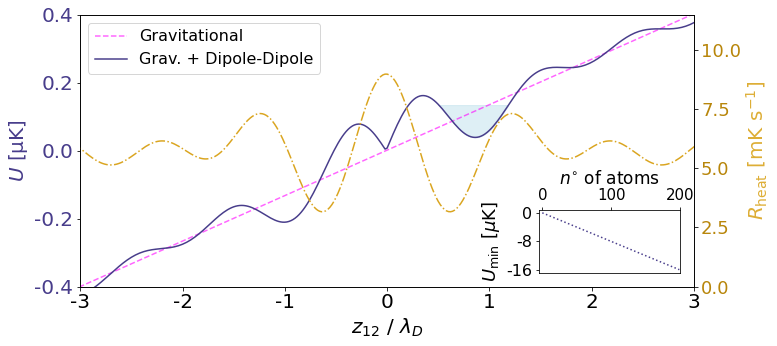
As we see from Fig.7, the size of the potential well created by the dipole-dipole interactions with a single atom is of the order of the recoil energy, possibly making trapping impractical. However, we can increase the trapping potential by increasing the number of atoms being driven. The general interaction Hamiltonian $H^{\prime}_{A}$ with $N_{i}$ driven atoms on the top of the optical system shown in Fig. 5 is

$$H_{A}^{\prime}=-\sum_{i}^{N_{i}}J^{\text{R}}_{i,A2}\left(\hat{\sigma}_{+}^{(i)}\hat{\sigma}_{-}^{(2)}+\hat{\sigma}_{+}^{(2)}\hat{\sigma}_{-}^{(i)}\right).$$

(38)

We see that the dipole-dipole potential increases linearly with the number of atoms, as seen from the inset of Fig. 7. Although such scenario can greatly improve the effects of dipole-dipole interactions due to its collective nature, one would have to carefully consider near-field interactions among atoms on the same side of the lens. Such scenario adds a complexity to the problem that is beyond the scope of this work, but which could be addressed with the presented mathematical formalism. Furthermore, a far-detuned atom trap based on dipole-dipole interactions could be in principle compatible with other near-resonance cooling techniques (as it can be inferred from Fig. 6), creating long-living optical traps.

In this work we have shown that resonant dipole-dipole interactions between two atoms can be amplified in the presence of a lens. Deriving a master equation for the dynamics of two driven atomic dipoles placed near the foci of an aplanatic lens system, we evaluate the modified dispersive and dissipative interactions between the dipoles, demonstrating a lensing effect in their coupling (Fig. 4). We also illustrate that the dipole-dipole coupling increases with an increasing numerical aperture of the lens, and analyze the dependence of the lens mediated dipole-dipole interaction on the atomic polarization. Such modified dipole-dipole interactions can be used, for example, to create a mutual trapping potential for atoms. We demonstrate such a trap potential for the case of an atom interacting with a weakly driven atom via an aplanatic lens (Fig. 7), estimating the limitations to the trap lifetime due to recoil heating, which could be mitigated by the collectively enhanced potential of $N$ weakly driven atoms.

The present results open a new avenue for engineering long-ranged dipole-dipole interactions in quantum optical systems, facilitating strong resonant dipole-dipole coupling while avoiding the detrimental near-field effects common in nanophotonics platforms. Lens-mediated dipole-dipole interaction could allow for self-organization of remote atomic systems, where external driving fields can control the dipoles oscillation phases to tailor their amplitude and mutual correlations. The general description of an aplanatic lens presented here encompasses the case of light propagation through a long optical fiber coupled to a lens on each end, a suitable platform for long distance dipole-dipole interfacing. One can consider an extension of the present scheme to a network of lenses and atoms where one can tailor collective multi-atom interactions in long-ranged systems with lenses. Such lens-modified collective dipole-dipole interactions would increase the versatility and modularity of quantum optical systems.

This work was supported by CONICYT-PAI 77190033 and FONDECYT 11200192 from Chile.

References

- Bakr et al. (2009) W. S. Bakr, J. I. Gillen, A. Peng, S. Fölling, and M. Greiner, Nature 462, 74 (2009).
- Cheuk et al. (2015) L. W. Cheuk, M. A. Nichols, M. Okan, T. Gersdorf, V. V. Ramasesh, W. S. Bakr, T. Lompe, and M. W. Zwierlein, Phys. Rev. Lett. 114, 193001 (2015).
- Parsons et al. (2015) M. F. Parsons, F. Huber, A. Mazurenko, C. S. Chiu, W. Setiawan, K. Wooley-Brown, S. Blatt, and M. Greiner, Phys. Rev. Lett. 114, 213002 (2015).
- Haller et al. (2015) E. Haller, J. Hudson, A. Kelly, D. A. Cotta, B. Peaudecerf, G. D. Bruce, and S. Kuhr, Nature Physics 11, 738 (2015).
- Yamamoto et al. (2016) R. Yamamoto, J. Kobayashi, T. Kuno, K. Kato, and Y. Takahashi, New Journal of Physics 18, 023016 (2016).
- Endres et al. (2016) M. Endres, H. Bernien, A. Keesling, H. Levine, E. R. Anschuetz, A. Krajenbrink, C. Senko, V. Vuletic, M. Greiner, and M. D. Lukin, Science 354, 1024 (2016).
- Barredo et al. (2016) D. Barredo, S. de Léséleuc, V. Lienhard, T. Lahaye, and A. Browaeys, Science 354, 1021 (2016).
- Kaufman and Ni (2021) A. Kaufman and K.-K. Ni, Nature Physics 17, 1324 (2021).
- Chin et al. (2017) Y.-S. Chin, M. Steiner, and C. Kurtsiefer, Nature Communications 8, 1200 (2017).
- Bianchet et al. (2021) L. C. Bianchet, N. Alves, L. Zarraoa, N. Bruno, and M. W. Mitchell, “Manipulating and measuring single atoms in the maltese cross geometry,” (2021), arXiv:2103.05783 [physics.atom-ph] .
- Robens et al. (2017) C. Robens, S. Brakhane, W. Alt, F. Kleißler, D. Meschede, G. Moon, G. Ramola, and A. Alberti, Opt. Lett. 42, 1043 (2017).
- Asenjo-Garcia et al. (2017) A. Asenjo-Garcia, M. Moreno-Cardoner, A. Albrecht, H. J. Kimble, and D. E. Chang, Phys. Rev. X 7, 031024 (2017).
- Sinha et al. (2020a) K. Sinha, P. Meystre, E. Goldschmidt, F. K. Fatemi, S. L. Rolson, and P. Solano, Phys. Rev. Lett. 124, 043603 (2020a).
- Sinha et al. (2019) K. Sinha, P. Meystre, and P. Solano, Nanophotonic Materials, Devices, and Systems 11091, 53 (2019).
- Dinc and Braǹczyk (2019) F. Dinc and A. M. Braǹczyk, Phys. Rev. Research 1, 032042(R) (2019).
- Calajó et al. (2019) G. Calajó, Y.-L. L. Fang, H. U. Baranger, and F. Ciccarello, Phys. Rev. Lett. 122, 073601 (2019).
- Sheremet et al. (2021) A. S. Sheremet, M. I. Petrov, I. V. Iorsh, A. V. Poshakinskiy, and A. N. Poddubny (2021).
- Trivedi et al. (2021) R. Trivedi, D. Malz, S. Sun, S. Fan, and J. Vučković, Phys. Rev. A 104, 013705 (2021).
- Buonaiuto et al. (2021) G. Buonaiuto, F. Carollo, B. Olmos, and I. Lesanovsky, Phys. Rev. Lett. 127, 133601 (2021).
- Poshakinskiy and Poddubny (2021) A. V. Poshakinskiy and A. N. Poddubny, Phys. Rev. Lett. 127, 173601 (2021).
- Pivovarov et al. (2021) V. A. Pivovarov, L. V. Gerasimov, J. Berroir, T. Ray, J. Laurat, A. Urvoy, and D. V. Kupriyanov, Phys. Rev. A 103, 043716 (2021).
- Jones et al. (2020) R. Jones, G. Buonaiuto, B. Lang, I. Lesanovsky, and B. Olmos, Phys. Rev. Lett. 124, 093601 (2020).
- Arranz Regidor et al. (2021) S. Arranz Regidor, G. Crowder, H. Carmichael, and S. Hughes, Phys. Rev. Research 3, 023030 (2021).
- van Loo et al. (2013) A. F. van Loo, A. Fedorov, K. Lalumiére, B. C. Sanders, A. Blais, and A. Wallraff, Science 342, 1494 (2013).
- Solano et al. (2017) P. Solano, P. Barberis-Blostein, F. K. Fatemi, L. A. Orozco, and S. L. Rolston, Nat. Commun. 8, 1857 (2017).
- Kim et al. (2018) J.-H. Kim, S. Aghaeimeibodi, C. J. K. Richardson, R. P. Leavitt, and E. Waks, Nano Letters 18, 4734 (2018).
- Newman et al. (2018) W. D. Newman, C. L. Cortes, A. Afshar, K. Cadien, A. Meldrum, R. Fedosejevs, and Z. Jacob, Science Advances 4, 5278 (2018).
- Boddeti et al. (2022) A. K. Boddeti, J. Guan, T. Sentz, X. Juarez, W. Newman, C. Cortes, T. W. Odom, and Z. Jacob, Nano Letters 22, 22 (2022).
- Fermani et al. (2007) R. Fermani, S. Scheel, and P. L. Knight, Phys. Rev. A 75, 062905 (2007).
- Yeung and Gustafson (1996) M. S. Yeung and T. K. Gustafson, Phys. Rev. A 54, 5227 (1996).
- Scheel et al. (2005) S. Scheel, P. K. Rekdal, P. L. Knight, and E. A. Hinds, Phys. Rev. A 72, 042901 (2005).
- Rekdal et al. (2004) P. K. Rekdal, S. Scheel, P. L. Knight, and E. A. Hinds, Phys. Rev. A 70, 013811 (2004).
- Skagerstam et al. (2006) B.-S. K. Skagerstam, U. Hohenester, A. Eiguren, and P. K. Rekdal, Phys. Rev. Lett. 97, 070401 (2006).
- Sagué et al. (2007) G. Sagué, E. Vetsch, W. Alt, D. Meschede, and A. Rauschenbeutel, Phys. Rev. Lett. 99, 163602 (2007).
- Goldstein and Meystre (1997) E. V. Goldstein and P. Meystre, Phys. Rev. A 56, 5135 (1997).
- Milonni and Knight (1974) P. W. Milonni and P. L. Knight, Phys. Rev. A 10, 1096 (1974).
- Sinha et al. (2020b) K. Sinha, A. González-Tudela, Y. Lu, and P. Solano, Phys. Rev. A 102, 043718 (2020b).
- Dung et al. (2002) H. T. Dung, L. Knöll, and D.-G. Welsch, Phys. Rev. A 66, 063810 (2002).
- Kobayashi et al. (1995) T. Kobayashi, Q. Zheng, and T. Sekiguchi, Phys. Rev. A 52, 2835 (1995).
- Goldstein et al. (1996) E. V. Goldstein, P. Pax, and P. Meystre, Phys. Rev. A 53, 2604 (1996).
- El-Ganainy and John (2013) R. El-Ganainy and S. John, New Journal of Physics 15, 083033 (2013).
- Agarwal and Gupta (1998) G. S. Agarwal and S. D. Gupta, Phys. Rev. A 57, 667 (1998).
- Hopmeier et al. (1999) M. Hopmeier, W. Guss, M. Deussen, E. O. Göbel, and R. F. Mahrt, Phys. Rev. Lett. 82, 4118 (1999).
- Haugland et al. (2021) T. S. Haugland, C. Schäfer, E. Ronca, A. Rubio, and H. Koch, The Journal of Chemical Physics 154, 094113 (2021).
- John and Quang (1995) S. John and T. Quang, Phys. Rev. A 52, 4083 (1995).
- Bay et al. (1997a) S. Bay, P. Lambropoulos, and K. Mølmer, Phys. Rev. Lett. 79, 2654 (1997a).
- Bay et al. (1997b) S. Bay, P. Lambropoulos, and K. Mølmer, Phys. Rev. A 55, 1485 (1997b).
- Xie et al. (2003) S.-Y. Xie, Y.-P. Yang, H. Chen, and S.-Y. Zhu, Journal of Modern Optics 50, 83 (2003).
- Kurizki (1990) G. Kurizki, Phys. Rev. A 42, 2915 (1990).
- Cortes and Jacob (2017) C. L. Cortes and Z. Jacob, Nature Communications 8, 14144 (2017).
- Behunin and Hu (2010) R. O. Behunin and B.-L. Hu, Phys. Rev. A 82, 022507 (2010).
- Jones et al. (2018) R. Jones, J. A. Needham, I. Lesanovsky, F. Intravaia, and B. Olmos, Phys. Rev. A 97, 053841 (2018).
- Sinha et al. (2018) K. Sinha, B. P. Venkatesh, and P. Meystre, Phys. Rev. Lett. 121, 183605 (2018).
- Yang et al. (2020) L.-P. Yang, C. Khandekar, T. Li, and Z. Jacob, New Journal of Physics 22, 023037 (2020).
- Varada and Agarwal (1992) G. V. Varada and G. S. Agarwal, Phys. Rev. A 45, 6721 (1992).
- de Léséleuc et al. (2017) S. de Léséleuc, D. Barredo, V. Lienhard, A. Browaeys, and T. Lahaye, Phys. Rev. Lett. 119, 053202 (2017).
- Pedrotti et al. (2006) F. Pedrotti, L. S. Pedrotti, and L. M. Pedrotti, Introduction to Optics (Pearson Education, 2006) p. 448.
- Gruner and Welsch (1996) T. Gruner and D.-G. Welsch, Phys. Rev. A 53, 1818 (1996).
- Buhmann and Welsch (2007) S. Y. Buhmann and D.-G. Welsch, Progress in Quantum Electronics 31, 51 (2007).
- Buhmann (2012a) S. Y. Buhmann, Dispersion Forces I (Springer-Verlag, Berlin, Heidelberg, 2012).
- Buhmann (2012b) S. Y. Buhmann, Dispersion Forces II (Springer-Verlag, Berlin, Heidelberg, 2012).
- Breuer and Petruccione (2002) H.-P. Breuer and F. Petruccione, Theory of open quantum systems (Oxford University Press, New York, 2002).
- Chang et al. (2014) D. E. Chang, K. Sinha, J. M. Taylor, and H. J. Kimble, Nature Communications 5, 4343 (2014).
- Novotny and Hecht (2012) L. Novotny and B. Hecht, Principles of nano-optics (Cambridge University Press, Cambridge, 2012).
- Eldredge et al. (2016) Z. Eldredge, P. Solano, D. Chang, and A. V. Gorshkov, Phys. Rev. A 94, 053855 (2016).
- Chang et al. (2013) D. E. Chang, J. I. Cirac, and H. J. Kimble, Phys. Rev. Lett. 110, 113606 (2013).
- (67) D. A. Steck, "Cesium D Line Data," available online at http://steck.us/alkalidata, (revision 2.2.1, 21 November 2019).
- Hohenester (2019) U. Hohenester, Nano and Quantum Optics: An Introduction to Basic Principles and Theory (Springer, Switzerland, 2019).