Extracting information on black hole horizons

The horizon is a paramount feature of black holes (BHs) entering in numerous astrophysical processes and in the understanding of the physics and geometry bordering quantum gravity. The Event Horizon Telescope¹¹ 1 https://eventhorizontelescope.org/. (EHT) has produced in 2019 the first BH image, the black hole’s shadow, as a bright ring–like structure with a central dark diskETH1. More recently, the EHT collaboration has shown the presence of a polarised fraction of light in the M87 galaxy, close to the BH boundary, measuring for the first time light polarisation which is interpreted as a sign of magnetic fields presence ETH2; ETH3. This detection opens a very rich perspective for the analysis of matter and fields subject to BH gravitational stresses, particularly in the jets emission.

In this letter, we study the properties of BH horizons in the Kerr geometry by investigating photon orbits with orbital frequency (relativistic velocity) equal in magnitude to the horizons frequencies. The possible detection of these photons would provide information on the properties of the horizons. Such photon orbits are shown to exist especially in regions close to the BH rotational axis. We interpret the results in the more general framework of metric bundles (MBs), introduced in observers; remnants; Pugliese:2019efv; Pugliese:2019rfz; LQG-bundles; PS; bundle-EPJC-complete and connected to the structures considered in de-Felice-first-Kerr; de-Felice3; de-Felice-mass; de-Felice4-overspinning, and Chakraborty:2016mhx; Tanatarov:2016mcs and Mukherjee:2018cbu; Zaslavskii:2018kix; Zaslavskii:2019pdc.

In bundle-EPJC-complete in the wider context of the BHs and naked singularities correspondence, the metric bundles structure was studied in detail, considering metric bundles as curves in a given plane called the extended plane. In that context it was highlighted the possibility that a part of these structures evidences the presence of replicas purposed for the analysis of photon circular motion and the determination of some characteristics of the inner and outer BH horizons particularly close to the rotation axis. Here in Sec. (2) we provide the analysis and complete classification of the co-rotating and counter-rotating replicas of the horizons of the Kerr metric in the black holes spacetimes, then focusing on the spacial cases of the equatorial plane and the case of extreme Kerr BH. In Sec. (3) we discuss the results in the bundles frame, interpreting our results through these structures, commenting on the relevance of the results and their phenomenological consequences.

The Kerr geometry The Kerr geometry is an exact, asymptotically flat, vacuum solution of the Einstein equations, for an axisymmetric, stationary spacetime, with (ADM) mass parameter $M\geq 0$, rotational parameter (spin—specific angular momentum) $a\equiv J/M\in[0,M]$, where $J$ is the total angular momentum. For $a=0$, the spacetime is the limiting static and spherically symmetric Schwarzschild geometry. For $a=M$ the solution is known as Kerr extreme BH, for $a>M$ there are naked singularity solutions. For the purposes of this work, it is convenient to represent the Kerr geometry in Boyer-Lindquist coordinates as

where

where $\alpha=\sqrt{\Delta\Sigma/\mathcal{P}}$ is the lapse function and $\omega_{zamos}=2aMr/\mathcal{P}$ is the frequency of the zero angular momentum observer (ZAMOS). (In the following analysis, to simplify the discussion, when not otherwise specified we use geometrical units with $r\rightarrow r/M$ and $a\rightarrow a/M$.).

The inner and outer BH horizons are located at

and the inner and outer ergosurfaces in the Kerr geometry are the radii

respectively. We consider null-like circular orbits with rotational frequencies $\omega_{\pm}:{g}(\mathcal{L},{\mathcal{L}})=0$, defined from the Killing vector $\mathcal{L}=\xi^{t}+\omega\xi^{\phi}$, in terms of the stationary $\xi^{t}=\partial_{t}$ and axisymmetric $\xi^{\phi}=\partial_{\phi}$ Killing vector fields. The limiting frequencies (or relativistic velocities) $\omega_{\pm}$:

are also the limiting frequencies bounding the (time-like) stationary observers four-velocity. In this letter we use the relation $\omega_{\pm}(r_{\pm})=\omega_{H}^{\pm}$, where $\omega_{H}^{\pm}$ are the frequencies of the outer and inner Kerr horizons respectively. The null vector fields $\mathcal{L}_{H}^{\pm}\equiv\mathcal{L}(r_{\pm})=\xi^{t}+\omega_{H}^{\pm}\xi^{\phi}$ in fact define the horizons of the Kerr BH as Killing horizons (being generators of Killing event horizons). (For $a=0$, the horizon of the Schwarzschild BH is a Killing horizon with respect to the Killing field $\xi^{t}$, consequently the event, apparent, and Killing horizons coincide. ).

Quantity $\omega_{H}^{\pm}$, expressing the BH rigid rotation, regulates (with the BH surface gravity) the BH thermodynamic laws and The variation of the BH irreducible mass $\delta M_{irr}\geq 0$ constrained by $(\delta M-\delta J\omega^{+}_{H})\geq 0$ for a variation of mass and momentum.

We study the solutions of $g(\mathcal{L},\mathcal{L})=0$ associated to orbits with radius $r$, which are different from the horizon radii, but corresponding to a photon orbit with orbital frequency equal in magnitude to the frequency $\omega_{H}^{\pm}$ of the BH horizons, we define these orbits as horizons replicas. We consider the corotating, $a\omega>0$ and the counter-rotating $a\omega<0$ replicas with frequencies that are equal in magnitude to the horizon frequencies. Notice that $g(\mathcal{L},\mathcal{L})(a,-\omega)=g(\mathcal{L},\mathcal{L})(-a,\omega)$ and thus $g(\mathcal{L},\mathcal{L})(-a,-\omega)=g(\mathcal{L},\mathcal{L})(a,\omega)$.

Replicas therefore connect two null vectors, $\mathcal{L}(r_{q},a,\sigma_{q})$ and $\mathcal{L}(r_{p},a,\sigma_{p})$, where $r_{q}\neq r_{p}$ is an outer or inner Killing horizon and in general $\sigma_{p}\neq\sigma_{q}$. We analyze the two regions $r<r_{-}$ (inner region) and $r>r_{+}$ (outer region). It turns out that solutions exists on planes close to the BH rotation axis. To represent the solutions, it is convenient to introduce the planes $(\sigma_{v},\sigma_{z})$ and spins $(a_{l},a_{s})$ that are defined Eqs. (32,33,34,31) of the Appendix and represented in Fig. (1). We introduce also the replicas $(r_{n},r_{z})$ that are the solutions described in Eqs. (29) and (30). Moreover, we use the notation $r_{\mathcal{Q}}^{\mathbf{I}}$ and $r_{\mathcal{Q}}^{\mathbf{II}}$ to designate one and two replicas, respectively, which are solutions of the multi-parametric equation for the radius $r_{\mathcal{Q}}\in\{r_{n},r_{z}\}$.

The inequality $\omega_{+}>\omega_{-}$ is valid in general, except on the horizons. In the case $\omega_{+}=-\omega_{H}^{\pm}$, there are no solutions. More generally we classify the solutions as follows.

Corotating inner horizon replicas with $\omega_{+}=\omega_{H}^{-}$:

with $\sigma_{crit}=2\left(2-\sqrt{3}\right)\approx 0.536$. Alternatively,

Corotating inner horizons replicas with $\omega_{-}=\omega_{H}^{-}$:

Alternatively,

Corotating outer horizons replicas with $\omega_{+}=\omega_{H}^{+}$:

Corotating outer horizon replicas with $\omega_{-}=\omega_{H}^{+}$:

Counter-rotating inner horizons replicas with $\omega_{-}=-\omega_{H}^{-}$:

Solutions cannot be in the ergoreigon, $r\in[r_{\epsilon}^{-},r_{-}[\cup]r_{+},r_{\epsilon}^{+}]$. Then:

in this case $a\in]0,1]$ and $\sigma_{k}=2\left(8-3\sqrt{7}\right)$. Alternatively,

Counter-rotating outer horizons replicas with $\omega_{-}=-\omega_{H}^{+}$

Alternatively,

with $a_{crit}\equiv 0.5784M$.

We consider now the particular case of an extreme Kerr BH, $a=M$, and the situation on the equatorial plane $\sigma=1$. Then,

Extreme Kerr BH:

(Note the cases $\omega_{(\pm)}=\omega_{H}^{\pm}$ and $\omega_{-}=-\omega_{H}^{\pm}$).

The equatorial plane $\sigma=1$:

In remnants it was discussed the existence of two corotating orbits $r_{\pm}^{\pm}$ such that $\omega_{*}(r_{\pm}^{\pm})=\omega_{H}^{\pm}$, respectively, and $r_{-}^{-}<r_{-}<r_{+}<r_{+}^{+}$ (almost everywhere but at $a_{g}=0$ for the static spacetime and $a_{g}=M$ for the extreme Kerr BH). More in general here we find,

(note the cases $\omega_{\pm}=\omega_{H}^{\pm}$). We summarize the situation as follows.

Inner horizon counter-rotating replicas with $\omega=-\omega_{H}^{-}$:

Inner horizon corotating replicas with $\omega=\omega_{H}^{-}$:

Outer horizon counter-rotating replicas with $\omega=-\omega_{H}^{+}$:

Outer horizon corotating replicas with $\omega=+\omega_{H}^{+}$:

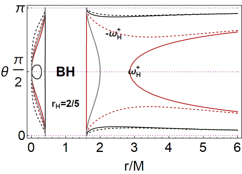
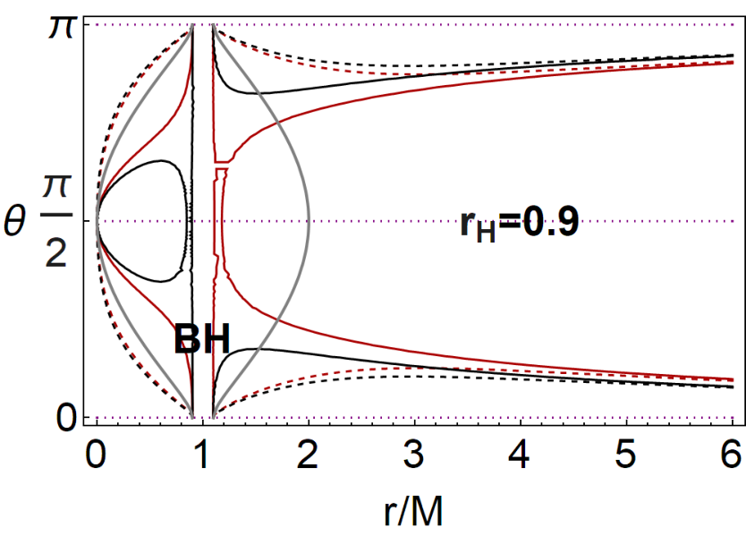
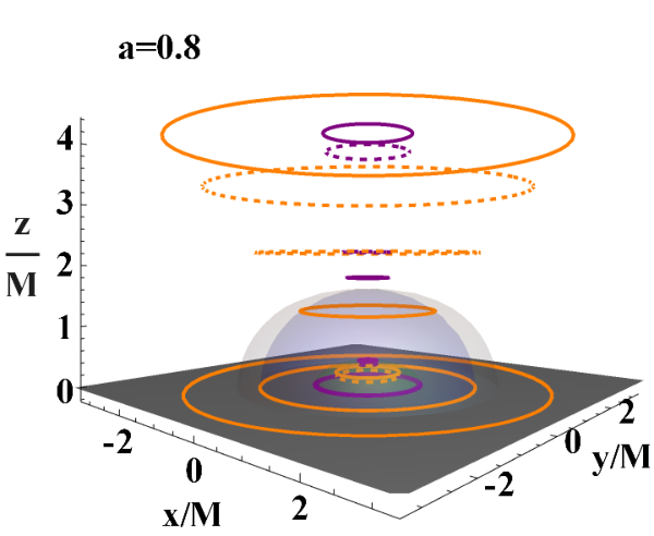
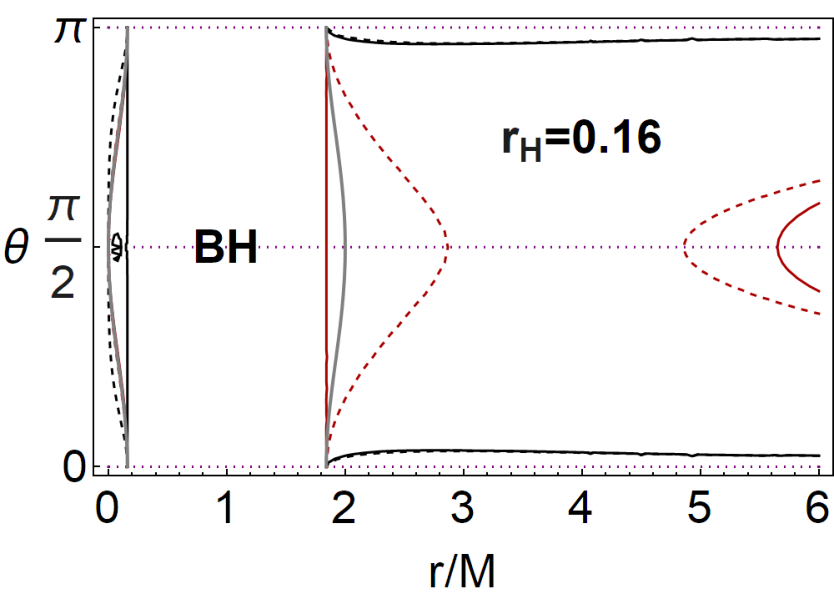
Examples of replicas are shown in Fig.  (1). To clarify this concept in Fig. (2), we show a set of replicas of the inner and outer horizons. A study of the asymptotic region is illustrated also in Fig. (1). As clear from Figs (1), there are two extreme values of $\theta$ for the existence of the inner horizon replicas in the outer region. A further interesting aspect is the asymptotic behavior (for large $r/M$), where the outer horizon and the curves representing the inner horizon replicas close and approach the BH poles (i.e., $\theta=\{0,\pi\}$, that is, for larger $r$ and small $\sigma$). For $r\rightarrow+\infty$ there is $\omega_{\pm}=0$. This means that at a fixed angle $\sigma$, the inner horizon replica approaches the outer horizon replica. Similarly, at a fixed radius $r/M$ and for values of $\theta$ approaching the BH poles, there are two replicas for two horizon frequencies, respectively. We note that for small $\sigma$ and large $r$ the two curves, inner and outer horizons replicas, get closer.

The replicas analysis of Sec. (2) evidences how every photon circular frequency $\omega$ can be read as a BH horizon frequency, and in this sense every photon circular orbit can be read as an horizon replica. Replicas can therefore be grouped in structures, known as metric Killing bundles (MBs) containing all (and only) the horizon replicas of every Kerr geometry, for a given (photon) frequency $\omega$, called bundle characteristic frequency. Therefore MBs also connect measures in different spacetimes, BH geometries and BH and naked singularities, grouping photon orbits in different geometries, characterized by equal value of the photon orbital frequency $\omega$. (Replicas in NSs were interpreted in remnants as “horizons remnants” and, more generally, appear connected to the "pre-horizon regime" introduced in de-Felice1-frirdtforstati; de-Felice-first-Kerr.). The connection between replicas and MBs appear evident by the MBs definition: MBs with characteristic frequency $\omega$ are solutions of the condition $a:\;g(\mathcal{L},\mathcal{L})=0$ for the fixed, constant $\omega$. Therefore we can read the results of Sec. (2) in terms of bundles properties.

MBs can be represented as curves on a plane, known as extended plane, tangent to the curve $a_{\pm}\equiv\sqrt{r(2M-r)}$, representing all the BHs horizons. The horizons curve $a_{\pm}>0$ is a functions of the horizons radii $r/M$ in the extended plane, for the inner BH horizons, where $r\in]0,M]$ (with $\omega=\omega_{H}^{-}\geq 1/2$), or the outer BH horizon, for $r\in[M,2M]$ (with $\omega=\omega_{H}^{+}\in]0,1/2]$). Introducing the quantify $\mathcal{A}=a\sqrt{\sigma}$, the extended plane of the Kerr geometry is the plane $\mathcal{A}/M-r/M$, or $a/M-r/M$ in the special case of the equatorial plane. (Note that the horizon curve is obviously independent of the polar angle $\theta$.). Using the variable $\mathcal{A}$ it is possible to connect points in different planes $\sigma$, as done in Sec. (2). The significance of the MBs with respect to the Kerr horizons lies in the fact that, per construction, each bundle is a curve tangent to the horizon curve in the extended plane. Consequently MB set must necessarily contain at least one BH geometry, and be tangent to only one BH geometry in the case of corotating frequency $\omega a>0$. For instance, the special bundle with characteristic frequency $\omega=1/2$, refers to the extreme Kerr BH spacetime as its tangent point to the horizon curve is $(r=M,a=M)$ with $\omega=\omega_{H}^{\pm}=1/2$ and, on the equatorial plane, where the extended plane is $a-r$, the metric bundle set contains the extreme Kerr BH only and NSs. In this sense, remarkably, the horizon curve in the extended plane is generated as envelope surface of all the MBs curves. The characteristic frequency of the bundles is therefore in particular the frequency of the BH horizon defined by the tangency point, hence each other point of the MB curve is its horizon replicas, and all the geometries of the curves are connected by this property. Regarding the representation of counter-rotating horizons replicas described in Eqs (11,12,13,14, 16,17,20,21,23, 24,25) in the extended plane, we note that, by using the symmetries of the $\mathcal{L}$ tensor and the Kerr metric tensor discussed in Sec. (2), we can represent counter-rotating replicas in a compact and immediate way by extending the extended plane into the negative region, with $\mathcal{A}<0$ (equivalently $a<0$). In this representation, the bundle characteristic frequency is always positive, and the curves extend, mostly continuously, in the negative section of the extended plane, at $a<0$, grouping corotating replicas of the horizon frequency in the positive sector $a>0$, and horizon counter-rotating replicas in the extension $a<0$. In this extension, the horizon curve is a circle of radius $M$ centered on the point $(a=0,r=M)$. Per construction the region ($a^{2}<a^{2}_{\pm}$ or $r\in]r_{-},r_{+}[$), bounded by the horizon curve, is inaccessible for the bundles which are not defined in this region. In this context, the inaccessibility of some frequencies for the observer (as for a part of the inner horizon curve frequencies), as concept of horizon confinement highlighted in Sec. (2), can be expressed in the MBs frame as “local causal ball”, that is a entirely confined region, inaccessible to any other region of the extended plane. Although we also consider also the inner region ($r<r_{-}$), in this analysis we are mostly interested in the information contained in the outer region $r>r_{+}$ and therefore accessible to the observer. The bundle curves with no portion in the outer region, are confined and the information is unaccessible for the observer.

Significantly then we can interpret results of Sec. (2) in the metric bundles framework. Replicas connect the inner region of the extended plane, bounded by the inner horizon, to the region outside the outer horizon. In this context we can explain how an observer can eventually measure a replica $\omega_{\circledast}$ of a BH horizon with spin $a_{\circledast}$ on the orbit $q_{\circledast}$. The point $q_{\circledast}$ belongs to the MB with characteristic frequency $\omega_{\circledast}$ which, in the observer spacetime $(a=a_{\circledast})$, crosses the point $q_{\circledast}$ and it is tangent to the observer BH horizon curve in the extended plane to the point ($a_{\circledast}$, $r_{\circledast}$). The replica registered by the observer is, as discussed in Sec. (2), the BH corotating or counter-rotating outer horizon frequency $\omega_{\circledast}=\pm\omega_{H}^{+}$ or the inner horizon frequency $\omega_{\circledast}=\pm\omega_{H}^{-}$. The stationary observer located at $q_{\circledast}$ has orbital frequency $\omega_{o}\in]\omega_{1},\omega_{2}[$, where $(\omega_{1},\omega_{2})$ are the limiting photon frequencies $\omega_{\pm}$, and one of the frequencies $(\omega_{1},\omega_{2})$ is the frequency $\omega_{\circledast}$ of the BH inner $r_{\circledast}=r_{-}(a_{\circledast})$ or outer horizon $r_{\circledast}=r_{+}(a_{\circledast})$, which is replicated on $q_{\circledast}$. The second light-like frequency of the pair $(\omega_{1},\omega_{2})=\omega_{\pm}$ is, according to Sec. (2), an horizon replica of a different BH with spin $a_{\odot}\neq a_{\circledast}$, included in the metric bundle with that characteristic frequency and tangent to the inner or outer BH horizon with spin $a_{\odot}$. The relation between the two frequencies $(\omega_{1},\omega_{2})=\omega_{\pm}$ on $q_{\circledast}$ is determined by a characteristic ratio, relating therefore also the BHs with spins $(a_{\odot},a_{\circledast})$. The two metric bundles with characteristic frequencies $(\omega_{1},\omega_{2})$ respectively cross on $q_{\circledast}$. (For a point $q_{\circledast}$ there is a maximum of two crossing bundles.).

We can express more precisely and in detail the relation between the replicas and bundle structure, with respect to the analysis of Sec. (2). The bundle curves have two notable points. In the extended plane the bundle has a tangent point $(a_{g},r_{g})$ on the horizon curve, defining the characteristic frequency of the bundle as horizon frequency. However, the bundle has also an origin, corresponding to the point at $r=0$ (the singularity limit in this frame). The horizon frequency is the characteristic frequency of the bundle and therefore the frequency at each point of the bundle, there is then at the bundle origin $a_{0}$ $(\mathcal{A}_{0})$ for $r=0$, defined as $a_{0}\equiv 1/\omega\sqrt{\sigma}$ (or $\mathcal{A}_{0}=a_{0}\sqrt{\sigma}=1/\omega$) . Replicas of a frequency $\omega$, studied in Sec. (2) in a fixed BH spacetime with spin $\bar{a}$, is provided by the point of the bundle crossing the horizontal lines $a=\bar{a}=$constant (or $\mathcal{A}=$constant, considering explicitly the dependence on the plane $\sigma$). Therefore it is a quantity dependent on the bundles curvature in the extended plane, as solutions of $a(\omega)=\bar{a}$, being $a(\omega)$ the bundles with characteristic frequency $\omega$.

Below we consider explicitly the relation between the frequency replicas, the bundles tangency condition to the horizon curve in the extended plane and the bundles origin spin. According to the value of $\sigma$, the inner horizon can be generated (tangent to the MB) either by MBs with naked singularities origins or with BH origins. A MB with BH origin generates only the inner horizon, this is because there is $\omega\equiv 1/\mathcal{A}_{0}\equiv 1/(a_{0}\sqrt{\sigma})\geq 1/a_{0}\geq 1$ (in magnitude) and therefore the relative bundle characteristic frequency is an inner horizon frequency (it is indeed a section of inner horizon curve in the extended plane, as the inner horizon frequencies are $\omega>1/2$, the case $\omega=1$ is therefore a discriminant case with $a_{g}/M=4/5,r_{+}/M=8/5,r_{-}/M=2/5$.). Or specifically we can summarize the relations between $(\omega,a_{0},\sigma)$ as follows:

On the other hand, as seen in Sec. (2) there are orbits with characteristic frequencies equal to the outer horizon frequencies, which are located in the inner region of the extended plane. A limiting special case is represented by the equatorial plane, $\sigma=1$, where the extended plane is $a-r$ and the bundles origin is $a_{0}=1/\omega$. This relevant case has been analyzed in Eqs ((19,20,21,22). We evidenced how MBs with BH origins are tangent to the inner horizon (for any plane $\sigma$), however for frequencies $\omega=\omega_{H}^{-}\geq 1$ with $a_{g}\in[0,0.8M]$ and tangent radius $r_{g}\in[0,2/5M]$, MBs are confined in the region of the extended plane upper-bounded by the inner horizon. Thus, more generally, for large values of $\sigma\in[0,1]$, and particularly on the equatorial plane MBs with BH origin spin $a_{0}$ are confined in the inner region of the extended plane. Consequently, on these planes $\sigma$s, all the frequencies $\omega\geq 1$ defining these bundles are confined and cannot be found in the outer region, i.e. $r>r_{+}$. Therefore, the confinement of the MBs tangent to the inner horizons can be overcomed, as noted in Sec. (2), by considering that the zero-quantity $g(\mathcal{L},\mathcal{L})$ depends explicitly on the plane $\sigma>0$ (and not from the bundle origin $\mathcal{A}_{0}$ only). For each point of the horizons curve, it is possible to find a replica for a plane $\sigma$ bounded in $\sigma<\sigma_{crit}$. This implies that close to the rotational axis, $\sigma\ll 1$, for a spacetime with spin $a$ it is possible to find an inner horizon replica in the outer region $r>r_{+}$. Consequently, bundles can extract “information” on the inner horizons frequencies near the rotation axis and, therefore, in this sense, the inner region is not entirely confined. Another significant aspect of the horizon confinement concerns the intriguing possibility of extracting information from counter-rotating orbits, while from the observational view-point, we established that the rotational axis of a Kerr BH may contain important information about the singularity and horizons.

This work was partially supported by UNAM-DGAPA-PAPIIT, Grant No. 114520, Conacyt-Mexico, Grant No. A1-S-31269, and by the Ministry of Education and Science of Kazakhstan, Grant No. BR05236730 and AP05133630.

References

• (1) The Event Horizon Telescope Collaboration et al, ApJL 875 (2019) L1
• (2) The Event Horizon Telescope Collaboration et al., ApJL 910 L12 (2021) 24.
• (3) The Event Horizon Telescope Collaboration et al., ApJL 910 (2021) L13.
• (4) D. Pugliese and H. Quevedo, Eur.Phys.J.C 81 3 (2021) 258.
• (5) C. Chakraborty, M. Patil, et al., Phys. Rev. D 95 8 (2017) 084024.
• (6) F. de Felice, Mont. Notice R. astr. Soc 252 (1991) 197-202.
• (7) F. de Felice, Class. Quantum Grav. 11 (1994) 1283-1292.
• (8) F. de Felice and L. Di G. Sigalotti, Ap.J. 389 (1992) 386-391.
• (9) F. de Felice and S. Usseglio-Tomasset, Class. Quantum Grav. 8 (1991) 1871-1880.
• (10) F. de Felice and S. Usseglio-Tomasset, Gen. Rel. Grav. 24 (1992) 10.
• (11) F. de Felice and S. Usseglio-Tomasset, Gen. Rel. Grav. 28 (1996) 2.
• (12) F. de Felice and Y. Yunqiang, Class. Quantm Grav. 10 (1993) 353-364.
• (13) S. Mukherjee and R. K. Nayak, Astrophys. Space Sci. 363 8 (2018) 163.
• (14) D. Pugliese and H. Quevedo, Eur. Phys. J. C 78 1 (2018) 69.
• (15) D. Pugliese and H. Quevedo, Eur. Phys. J. C 79 3 (2019) 209.
• (16) D. Pugliese and H. Quevedo, arXiv:1910.02808 [gr-qc] (2019).
• (17) D. Pugliese and H. Quevedo, arXiv:1910.04996 [gr-qc] (2019).
• (18) D. Pugliese and G. Montani, Entropy 22 402 (2020).
• (19) D. Pugliese and Z. Stuchlik, Class. Quantum Grav. https://doi.org/10.1088/1361-6382/abff97 (2021).
• (20) I. V. Tanatarov and O. B. Zaslavskii, Gen. Rel. Grav. 49 9 (2017) 119.
• (21) O. B Zaslavskii., Phys. Rev. D 98 10 (2018) 104030.
• (22) O. B. Zaslavskii, Phys. Rev. D 100 2 (2019) 024050.