On Dynamics of
Santanu Nandi
Abstract: This article discusses some topological properties of the dynamical plane (-plane) of the holomorphic family of meromorphic maps for . In the dynamical plane, we prove that there is no Herman ring, and the Julia set is a Cantor set for the maps when the parameter is in the unbounded hyperbolic component contained in the four quadrants in the complex plane. Julia set is connected for the maps when the parameters are in other hyperbolic components of the parameter plane.
Keywords: Fatou set; Julia set; periodic points; singular values; immediate basin; critical point; attracting domain.
1 Introduction
In this article we study the dynamics of the family of translated maps. We denote this family by . The dynamics of the transcendental meromorphic family of maps has been studied in [6], [7]. The dynamics of the family is much different than the dynamics of The origin is not a fixed point for the maps in the family , however the origin was always a super-attracting fixed point for the maps in the family The maps in are even, and the Fatou components of the maps in are symmetric about the origin.
For a meromorphic map, there are three possibilities for the iteration of an orbit. A point either has finite orbits (periodic points), terminates at a pole, or has infinite orbit under the iteration of the function. For a transcendental meromorphic function, for more than one pole, the pre-pole is defined by the set . By Picard’s Theorem the set is infinite. We need two very important tools, called Fatou set and Julia set to study the dynamics of the family of maps. The Fatou set or Stable set contains the points so that is defined and forms a normal family in a neighborhood of the point The set of points that are in the complement of the Fatou set is called the Julia set. Clearly, the Fatou set is open, the Julia set is closed and the set So is non-empty. One can easily see that the Fatou and Julia set are completely invariant.
We denote the singular point is the set of points such that the meromorphic function has no regular covering at the point. The value of the function at the point is called the singular value. If a singular value is algebraic, then it is called a critical value where as if it transcendental then it is called an asymptotic value. For an asymptotic value , an asymptotic tract is defined as the open set such that is a punctured neighborhood around The map in the family has two asymptotic values, and a critical value, the origin. The maps have four asymptotic tracts in each of the four quadrants.
We have arranged this paper as follows. In section 2, we have discussed some basic mapping properties of the maps in . In section 3, we give a classification of the stable components of the maps in and also proved that there is no Herman rings in the stable components for these maps. In section 4, we see that there are four unbounded hyperbolic components for which the the maps has a single attracting periodic points and all singular values are attracted by that attracting basin. We briefly introduced the symbolic dynamics and proved the main result of this article that the Julia set is Cantor set for a set of parameters in the parameter plane for the maps in .
2 Properties of the maps in
Consider the regions . It is clearly seen that for each defines hyperbola in the complex plane for Each open region bounded by two such curves, mapped to by The inverse map is given by the formula:
.
Hence the will be given by function. Therefore we must specify the branch of when defining the inverse map. We will denote the branches as in each of the region .
The zeros of the family of maps in is of the form for . We label the zeros of the family of maps on the real and imaginary axes respectively by even and odd numbers indexing. For , the zero lies on the real axis when whereas for and the zero lies on the negative real axis. Indexing along the imaginary axis can be done in a similar fashion for . Thus one can find zeros along real axis and along the imaginary axis.
Poles of the family of maps lies on the both real and imaginary axes and are given by for For positive and the pole is denoted by whereas for negative and the pole is denoted by . For , a similar indexing can be done for poles along the imaginary axis. Therefore one can find the poles of the family of maps of as along real axis and along the imaginary axis.
Lemma 2.1.
The maps and their derivatives in the family follow the symmetry property as below.
(i)
(ii)
Proof.
The proofs follow from the properties of conjugates of complex numbers.
∎
3 Classifications of the Fatou components
Let be a component of the Fatou set of the maps in The map maps the component to another component of the Fatou set. If the image set contains a singular value, then the map may not be onto. In any case we call the image component and that satisfy the following dichotomy:
(i) There exists integers such that . The component is called eventually periodic.
(ii) For all integers , , and the component is called wandering domain.
The qualitative and quantitative behavior of stable components of meromorphic maps are categorized by the nature of the periodic points. Suppose that be a periodic cycle. We define the multiplier or eigenvalue of the periodic points by . Suppose a stable component eventually land on the cycle . Then
(a) is attractive: Each domain contains a periodic point of the periodic cycle and the multiplier . Some domain in the cycle must contain a singular value. If the multiplier then the critical point itself is a periodic point in the cycle and the periodic cycle is called super-attractive.
(b) is parabolic: The multiplier map is of the form . The boundary of each component contains a periodic point of the cycle and the points in the domain are attracted to the periodic point. Some component must contain a singular value.
(c) is Siegel Disk: The multiplier map of the periodic cycle is given by where is an irrational number. There is a holomorphic homeomorphism from the domain to the unit disk , conjugating the first return map to an irrational rotation from to the unit disk .
(d) is Herman Ring: Each of the periodic components is holomophically homeomorphic to the standard annulus and the first return map is conjugate to an irrational rotation of the annulus by a holomorphic homeomorphism.
(e) is essentially parabolic or Baker Domain: The periodic domain contains a point ( possibly ) on its boundary so that for all but is not holomorphic in . If the
From [1], one can see that the maps in the has no essentially parabolic domain. The next theorem shows that there is no Herman ring in the stable set. Therefore stable set can only be classified by the first three types of components as discussed above.
Theorem 3.1.
There is no Herman ring in the Fatou set of .
Proof.
Let be a cycle of Herman rings. Each of this domain is conformally conjugate to an annulus. Let is a degree one self mapping on a domain . Let be a simple closed curve in . Then must encloses a pre-pole in the bounded region, say . Choosing and suitably, we can assume that passes very close to a pole and maps the bounded region to the complement of a bonded set. contains a pole say, .
We claim that contains . If not, by symmetry, there is an in . Therefore and both have non-zero winding number around the origin. So they must intersect, but they cannot. So contains both and This implies that the curve has a non-zero winding number around the origin and intersects at-least number of vertical strips defined in section 2. Therefore the winding number of is greater than contradicts that is degree one map.
∎
Lemma 3.2.
Let be an arbitrary small neighborhood of . Then has a non-empty intersection with if and only if is a pre-pole of .
Proof.
If is a pre-pole of , clearly Conversely, if would be a point of , then we can have a small neighborhood of that would be in , since is open. Therefore is in . Any small neighborhood of contains a pre-pole of because pre-poles are dense in Let be such neighborhood of and let be a pre-pole in . We can have a nested closed sets of neighborhoods of and a sequence of pre-poles with such that the infinite intersections of these closed nested sets is non-empty and contains a single point, namely . Clearly the sequence as By proposition 6.1 of [3], is a pre-pole of
∎
4 Hyperbolic components in the parameter space
One can find the proof of the following theorem in [2].
Theorem 4.1.
Let be a nonempty domain in a complex Banach space Let be a bounded holomorphic map. If lies strictly inside , then has a fixed point in .
We use the above theorem in the domain of real numbers to prove the following theorem.

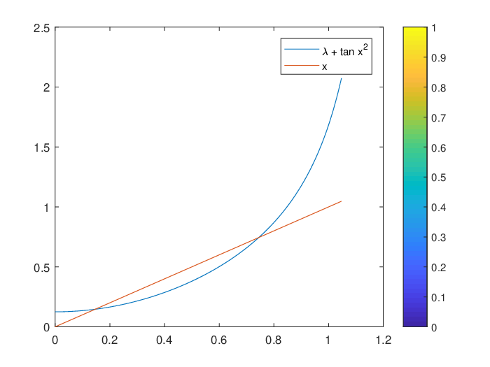
Theorem 4.2.
For and , the origin is attracted by an attracting cycle.
Proof.
If is in , the orbit of the origin belongs to . If the function has an attracting periodic fixed point, the attracting periodic points lie on To see the existence of a real fixed point of , we prove that the map is a contraction mapping in some bounded domain of The derivative is an increasing function in with By Lipschitz condition and Mean Value Theorem, there is such that for . Therefore has at-least a fixed point in the interval say . The multiplier map for the fixed point is given by For to be an attracting fixed point, we need to have implies or Therefore or .
Let be an attracting periodic cycle. For to be less than 1, we need to have This implies that for all with the function has an attracting fixed point with
As , one can check the orbit of the critical value is bounded by , i.e. . Clearly, the origin must be attracted by the attracting fixed point ∎

Lemma 4.3.
There are four unbounded regions in the four complex quadrants such that for all singular values of are attracted by an attracting fixed point.
Proof.
Let and is holomorphic in . Then, .
If then So there exists such that for all with , . Consider the region . So each of these regions is an unbounded region in each quadrant separated by a hyperbola in the complex plane.
For each asymptotic value (or ) in , consider a ball for some (or . We will show that for each Since is a Banach space, by Theorem 4.1, has an attracting fixed point inside the ball . for suitably chosen in . Therefore, for any has an attracting fixed point. However, the attracting basin of the attracting cycle contains the origin because is in and is the image of the origin under The orbit of the other asymptotic value eventually land on the orbit of (or ) and hence in the corresponding attracting basin of .
∎
Theorem 4.4.
If , Julia set of is a Cantor set and the Julia set is topologically conjugate to shift automorphism
To prove the theorem we need to introduce the concept of shift space. Let be the set of alphabet and consider the space of infinite sequences from to Denote an element x in the space as x . Let us denote to be a finite word with . We define a metric as the following:
In other words, two points and are at distance if they agree at their -central blocks.
The topology induced by this metric is equivalent to the topology defined in [5]. Define the shift map by . The map has the following properties. We refer to [4] for more detail.
Lemma 4.5.
is a compact metric space.
Lemma 4.6.
is a homeomorphism.
Theorem 4.7.
The set is a Cantor set.
Lemma 4.8.
If , there is one multiply connected unbounded Fatou set.
Proof.
Without loss of generality we can assume that is in the unbounded component and be the Fatou component containing the attracting fixed point of . and must contain a singular value. Without loss of generality we can assume that is in We claim that all other singular values are in . Choose a sufficiently large with such that for sufficiently large. Then a small neighborhood around contains . If necessary by making large, we can get a ball such that . Therefore, for with for sufficiently large , is in the the unbounded Fatou component containing the periodic point. We have that each of the for , are conformally conjugate and preserves the dynamics. So the singular value is in the Fatou component containing and the periodic fixed point for .
Define a path such that and . Each branch of is an infinite path joining pre-zeros. So all pre-image must intersect the unbounded periodic Fatou component Then is completely invariant. Using lemma 4.3, we have that all singular values are in ∎
Proof.
Let denotes the set of post-singular points. Since all singular values are attracted to the attracting fixed point, we can enclose the post-singular points with a single set except for a finite number of points outside. Let the set of all singular and post-singular points. Let be the complement of in Then is a neighborhood of the points in the Julia set . All inverses of under is well defined and have infinitely many closed bounded components. Since infinity is an essential singularity and contained in , each of the bounded components contain a pole. Let denotes the bounded components indexed by the pole(describe the indexing). Denote the th pre-image of under by where denotes a vector defined as . Suitably choosing the branches, we can get a nested sequences of closed bounded sets, namely, such that for . Also note that diam tends to zero as Therefore each of the set is singleton and contains a point of the Julia set Note that and Since , for some we can conclude that is a totally disconnected set and .
Assign a point to a point in the set defined by such that , i.e. . In other word, the point should also satisfy . For a point with we consider . We need to show that is a bijection. Claim that if If not, there is such that There exist and such that . Let denotes a sequence defined as and denotes an inverse branch of . There exist two inverse branches so that with ( and ). Since and we can analytically extend these inverse branches to the set Consider the branches of so that and . By assumption both and are in implies that . Inductively all other branches of are also equal and that implies For and we have that Hence the map is an injection.

Let be an element in the sequence space . Let’s consider be the inverse branches of . For each of the inverse branch on consider the set Then each of the set is closed bounded set and the diameter tends to zero. Now choose the branches of on in such a way that . So we have . This is a sequence of nested closed sets with diameter of the sets tends to zero. Therefore the set is singleton and contains a point of So If , then is a prepole and a single point. Hence the map is onto.
Since and are compact and is a continuous bijection, the inverse map is also continuous.
If is a point in , there is a in so that That implies . Hence the map shifts the element of one unit to the right. On the other way, is uniquely determined by for the point So Therefore the map determines the point shifted one unit to the right, i.e. Hence the following diagram is commutative.
Thus is a Cantor set.
∎
Pictures of the parameter space give nice topological and combinatorial structure of the hyperbolic components. It will be interesting to see the bifurcation of the periodic cycle on the boundary of the bounded hyperbolic components. We plan to explore this further in our future work.
References
- Devaney and Keen [1989] R. L. Devaney and L. Keen. Dynamics of meromorphic maps : maps with polynomial schwarzian derivative. Annales scientifiques de l’École Normale Supérieure, Ser. 4, 22(1):55–79, 1989. doi: 10.24033/asens.1575. URL http://www.numdam.org/articles/10.24033/asens.1575/.
- Harris [2003] L. A. Harris. Fixed points of holomorphic mappings for domains in Banach spaces. Abstract and Applied Analysis, 2003(5):261 – 274, 2003.
- Keen and Kotus [1995] L. Keen and J. Kotus. Dynamics of the family lambda tan z. arXiv preprint math/9507225, 1995.
- Lind and Marcus [2021] D. Lind and B. Marcus. An introduction to symbolic dynamics and coding. Cambridge university press, 2021.
- Moser [(Princeton: Princeton University Press,1973] J. Moser. Stable and random motions in dynamical systems: With special emphasis on celestial mechanics. (Princeton: Princeton University Press,1973).
- Nandi [2020] S. Nandi. Dynamics of the family . Far East Journal of Dynamical Systems, 32(2):67–91, July 2020.
- Nandi [2021] S. Nandi. Combinatorial structure of the parameter plane of the family . Far East Journal of Dynamical Systems, 33(1):1–38, Jan. 2021.