Reduced scaling of optimal regional orbital localization via sequential exhaustion of the single-particle space
Abstract
Wannier functions have become a powerful tool in the electronic structure calculations of extended systems. The generalized Pipek-Mezey Wannier functions exhibit appealing characteristics (e.g., reaching an optimal localization and the separation of the - orbitals) when compared with other schemes. However, when applied to giant nanoscale systems, the orbital localization suffers from a large computational cost overhead when one is interested in localized states in a small fragment of the system. Herein we present a swift, efficient, and robust approach for obtaining regionally localized orbitals of a subsystem within the generalized Pipek-Mezey scheme. The proposed algorithm introduces a reduced workspace and sequentially exhausts the entire orbital space until the convergence of the localization functional. It tackles systems with 10000 electrons within 0.5 hours with no loss in localization quality compared to the traditional approach. Regionally localized orbitals with a higher extent of localization are obtained via judiciously extending the subsystem’s size. Exemplifying on large bulk and a 4-nm wide slab of diamond with NV- center, we demonstrate the methodology and discuss how the choice of the localization region affects the excitation energy of the defect. Furthermore, we show how the sequential algorithm is easily extended to stochastic methodologies that do not provide individual single-particle eigenstates. It is thus a promising tool to obtain regionally localized states for solving the electronic structure problems of a subsystem embedded in giant condensed systems.
keywords
regionally localized orbitals, Pipek-Mezey Wannier functions, nitrogen-vacancy center1 Introduction
Localized orbitals are widely used in electronic structure computations for multiple purposes: conceptually, they can provide valuable information about chemical bonding and chemical properties of molecules and materials. More importantly, they allow the evaluation of non-local two-body interaction integrals at a significantly reduced cost due to the reduced spatial overlaps. Hence, they represent a powerful tool in mean-field and post-mean-field electronic structure calculations such as hybrid functional calculationsWu et al. 2009; Gygi and Duchemin 2013, density functional theory with the Hubbard correction termMiyake et al. 2009; Tomczak et al. 2009, or many-body caluations.Choi et al. 2012; Weng and Vlček 2021 In the same vein, the maximally localized orbital descriptions is optimal for treating correlation phenomena since (due to the locality) the number of “inter-site” interactions is minimal, and the effective size of the problem is smaller. As a result, optimally localized states are essential in the context of embedding and downfolding for many-electron problemsAryasetiawan et al. 2009; Pavarini et al. 2011; Bowler and Miyazaki 2012; Lau et al. 2021.
Arguably, the most popular approaches to obtain localized states are the Foster-Boys (FB) scheme Boys 1960; Foster and Boys 1960 for molecules and the maximally-localized Wannier functions (MLWF)Marzari and Vanderbilt 1997; Marzari et al. 2012 for periodic solids. In addition, selected columns of the density matrix (SCDM)Damle et al. 2015 localization scheme provides an alternative to find a localized basis,Damle et al. 2017; Damle and Lin 2018; Damle et al. 2019; Vitale et al. 2020 which however avoids the localization optimization. Among these and other orbital localization schemesEdmiston and Ruedenberg 1963; Edmiston and Ruedenberg 1965; Löwdin 1966; von Niessen 1972; Damle et al. 2015, the Pipek-Mezey (PM) localized molecular orbitals Pipek and Mezey 1989 are appealing due to their high spatial localization and (conceptually) the separation of characters of chemical bonds. Recently, PM localized molecular orbital formalism has been expanded to periodic systemsJónsson et al. 2017. This generalized Pipek-Mezey Wannier Functions (G-PMWF) approach retains the advantages (particularly stronger localization) compared with MLWF.
The iterative optimization, however, translates to a high computational cost Pipek and Mezey 1989 and requires that all single-particle states are known. This becomes a bottleneck for giant systems: the overhead is substantial when one is interested only in a small portion of the otherwise giant system, such as maximally localized orbitals associated with a point defect in solids, an adsorbate molecule on a surface, or molecular states in a complex environment. Here, it is still often necessary to handle the entire problem, despite only a fraction of localized states being sought. Such nanoscale problems involve thousands of electrons and the prevalent strategy is to lower the number of iteration steps necessary to reach the optimum, e.g., by a robust solverClement et al. 2021. Although the proposed scheme can effectively lower the iteration steps towards convergence, a minimal atomic orbital basis is still required for determining the atomic charges. Further, for truly giant systems, one would employ techniques that avoid the use (or knowledge) of all single-particle statesBaer et al. 2013; Cytter et al. 2018; Chen et al. 2019; Fabian et al. 2019; Nguyen et al. 2021; Baer et al. 2022; Neuhauser et al. 2013; Romanova and Vlček 2022; Neuhauser et al. 2013; Ge et al. 2014; Neuhauser et al. 2017; Dou et al. 2019; Takeshita et al. 2019; Neuhauser et al. 2014; Vlček et al. 2017; Vlček et al. 2018; Romanova and Vlček 2020; Vlcek 2019.
Herein, we present a new and complementary top-down approach leading to a fast, efficient, and robust orbital localization algorithm via sequentially exhausting the entire orbital space. It is beneficial for obtaining regionally localized orbitals for a subsystem within the G-PMWF scheme. In contrast to other methods, the problem’s dimensionality is reduced from the outset by partitioning the orbital space. As our work space is effectively compressed, the dimensionality of the relevant matrices in the G-PMWF scheme is much smaller and therefore, the time per iteration step is shortened by orders of magnitude. The unitary transform is performed iteratively till convergence. The transformation starts directly either with: (i) the canonical delocalized orbitals without any external or auxiliary atomic basis setZhang and Li 2014; Clement et al. 2021; or (ii) initial guess of the subspace of localized single-particle orbitals (which can be obtained by, e.g., by filteringBaer et al. 2013; Chen et al. 2019; Fabian et al. 2019; Baer et al. 2022; Neuhauser et al. 2014; Vlček et al. 2018). The compression of dimensionality helps to reduce the scaling of the method with the number of electrons to be linear. The completeness of sequentially exhausting the orbital space is demonstrated by the converged localization functional. We further test the quality of the localized basis by constructing an effective Hubbard model for the NV- defect center in diamond and computing its optical transition energies in bulk supercells and a giant (4 nm thick) slab containing nearly 10000 electrons. Excellent agreement between the sequential exhausting approach and the full space approach is achieved for the computation of optical transition energies. The accuracy of Hubbard model calculations is further improved by the Wannier function basis obtained from the subsystem with an extended size. In the last section, we provide a thorough discussion on how the choice of localization affects the excitation energies of the embedded NV- center.
2 Theory
2.1 Generalized Pipek-Mezey Wannier Functions
In this subsection, we briefly revisit the G-PMWF formalismJónsson et al. 2017 to clarify the motivation for this work. The G-PMWF evaluates the orbital localization using the following quantity as a functional of the unitary matrix U:
| (1) |
Here, denotes the state, and represents the number of states that spans a particular orbital space. denotes the atom in the system, and is the number of atoms in the system. is termed the atomic partial charge matrix (defined below). In practice, represents the partial charge on atom contributed by state . The stationary point of corresponds to the unitary matrix U that transforms the canonical states into Pipek-Mezey localized states
| (2) |
where represents the canonical state.
Generally, the value of is iteratively maximized till reaching convergence. In the iteration step, the matrix is defined as
| (3) |
Here represents either the transformed state (0) or the canonical state (=0). In real-space representation, denotes the atomic weight functionHirshfeld 1977; Cioslowski 1991; Bader 1994; Alcoba et al. 2006; Lillestolen and Wheatley 2008; Lillestolen and Wheatley 2009; Knizia 2013; Janowski 2014; Lehtola and Jónsson 2014; Knizia and Klein 2015 in replacement of the Mulliken partial charge schemePipek and Mezey 1989.
For , the matrix can also be calculated by
| (4) |
Note that in practice, the matrix has a dimensionality of . The number of elements can rocket to 109 for a system with 103 atoms with occupied states. Furthermore, the theoretical scaling of the method is ( denotes the number of grid points in real-space). Our numerical results for the defect center in diamond are close to this theoretical behavior, as discussed in the Results and Discussion section.
2.2 Sequential Variant of G-PMWF
This subsection presents an efficient algorithm to obtain a subset of PMWFs localized on a specific set of atoms.
2.2.1 Fragmentation treatment
Conventionally, one has to localize all states and then identify states that are regionally localized on the selected atoms. For instance, for a molecule surrounded by other atoms/molecules, will be four if considering only the valence electrons and doubly occupancy. When , this approach suffers from a significant overhead. This is quite limiting when nanoscale systems are considered: the dimensionality of matrix and the computational scaling make it challenging to work with thousands of electrons. Previously, we introduced a modified form of the PM functional to account for () selected atoms only and search for the states directlyWeng and Vlček 2021 . Such a modification is equivalent to the search of a local maximum of on the selected atoms, and it reduces the dimensionality to . In this work, we further compress the to simply 1 by creating a single fragment from the subset of atoms. Unlike the “fragment” proposed in the FB schemeZhang and Li 2014, our definition of a fragment is defined using the atomic weight function
| (5) |
where denotes the fragment of interest. The functional thus becomes
| (6) |
where is the modified PM functional for the fragment.
Note that: (i) the unitary transform is still performed on all states that need to be known, and (ii) the states are identified from by evaluating the partial charge on the selected fragment. In this context, we define the measure of the locality of a specific state on the fragment as
| (7) |
Its value ranges from 0 (not localized) to 1 (most localized). Only the top states of the states in the decreasing order of are considered the regionally localized Wannier functions on the fragment.
Next, the G-PMWF approach is broken into two steps: (1) maximize (Eq.(6)) and find the states that are localized on the fragment; (2) maximize the canonical (Eq.(8)) using the states from step 1 and obtain localized states on each individual atom of the fragment.
| (8) |
Essentially, the first step is a “folding” step where the electron density is effectively localized on the fragment disregarding the individual atoms. The second step is instead an “unfolding” step where the electronic states obtained from step 1 are unfolded onto each individual atom in the fragment.
The matrix is reduced to in step 1 and to in step 2, respectively. The second step is trivial in cost since is often much smaller than . However, the first step can still be expensive when working with thousands of electrons and the knowledge of eigenstates is necessary.
2.2.2 Sequential exhausting of the full orbital space
To further compress the in the maximization process and, in principle, avoid the knowledge of states altogether, we introduce a sequential variant of G-PMWF, sG-PMWF. We first review the approach which assumes states are available, and at the end of this section, we extend it to a more generalized case when the eigenstates do not need to be known a priori.
The sG-PMWF approach incorporates an additional iterative loop (“outer-loop”) to successively maximize the functional . The idea is schematically presented in Figure 1. A generalized original (entire) space, either occupied or unoccupied, is spanned by orthonormal canonical states. The initial matrix that contains the canonical states is an identity. Each row of the matrix contains the coefficients of a single-particle state in the canonical basis. The number of rows represents the number of states used in the matrix. The black lines and arrows stand for the initialization of the localization procedure. The outer-loop is guided by the blue lines and arrows, while the magenta lines and arrows guide the inner-loop (maximizer). The red points denote the convergence checkpoints.
Our goal is to find only states that are spatially localized on a selected fragment, and we seek to minimize the cost of the calculation by neglecting the localization in the other regions of the systems. The general procedure is as follows:
First, we assume that in practical calculations, it may be necessary to account for a “buffer,” i.e., we search for states (where is typically similar to in magnitude). We denote the most localized orbitals chosen based on the value of (Eq. 7) as “core states”. And the “core space” is spanned by such states. The original space is essentially split into two, the core and its complement space (denoted “rest space”). The states in the rest space are then reordered upon their locality for the next step.
Second, a work space is built with a dimensionality of , where . The first part of the work space is filled by the core states (the yellow region). On the other hand, the rest space is partitioned into blocks according to the value of , which is an arbitrary number ( 1) that denotes the number of states from the rest space. And note that the states in the rest space have been re-ordered in the decreasing order of . The number of states in each block satisfies the following equations
| (9) |
and
| (10) |
Here represents the number of states in the block. The rest space is sequentially updated (explained in the next step) and can be re-accessed during the localization process. The index denotes and iteration step in the outer-loop and the and are connected by
| (11) |
Third, the initial (=0) objective functional value (Eq. (6)) is calculated for the work space and the change of the PM functional in the outer-loop is defined as
| (12) |
The convergence checkpoint 1 in Figure 1 evaluates the as well as the accumulative step . The iteration will exit the outer-loop if either
| (13) |
or
| (14) |
is satisfied. The convergence threshold 1 and the maximal outer-loop iterations are carefully chosen to converge the localization (see the next section). If the iteration does not exit the loop, the index will become , and the corresponding (Eq. 11) block will fill the second part of the work space. The constructed work space then enters the maximization solver (the inner-loop in magenta). The change of the PM functional in the inner-loop is defined as
| (15) |
Here denotes the iteration step (if iterative maximization is needed) in the inner-loop. The convergence checkpoint 2 evaluates the as well as the accumulative step . The iteration will exit the inner-loop if either
| (16) |
or
| (17) |
is satisfied. The convergence threshold 2 and the maximal inner-loop iterations are carefully chosen to allow the work space to reach the maximum smoothly (see the next section). Once exiting, the core space is identified from the transformed work space, and the residues of work space replace the states in the block. This operation is denoted “the update of the rest space” since both the core and rest spaces are dynamic during the maximization. The index is reset to 0, and the arrives at the convergence checkpoint 1. If the iteration does not exit the loop, the next block then fills the work space to re-enter the maximizer. With all the blocks exhausted and updated, the states in the rest space will be re-ordered again for the re-access.
In practice, the outer-loop (identify the core space, construct the work space, maximization, and update the rest space) has to be iterated multiple times until the is converged. In general, each iteration step in the outer-loop feeds the core space with the ingredients to localize itself and sequentially exhaust the full orbital space until convergence. However, the cost of the calculation depends primarily on the size of the work space . A small might require extra outer-loop iterations, but the cost of each maximization (“inner-loop”) should be orders of magnitude smaller than the traditional full-space approach.
So far, we have assumed that a basis of individual single-particle states is known (e.g., obtained by a deterministic DFT). However, this procedure is trivially extended even to other cases, e.g., when stochastic DFT is employedBaer et al. 2013; Cytter et al. 2018; Chen et al. 2019; Fabian et al. 2019; Nguyen et al. 2021; Baer et al. 2022. For simplicity (and without loss of generality), we assume the localization is performed in the occupied subspace. Here, the sG-PMWF calculation is initialized by constructing a guess of random vectors which are projected onto the occupied subspace as . These random states then enter the core space in Figure 1. Here, the projector is a low-pass filter constructed from the Fermi operator leveraging the knowledge of the chemical potentialBaer et al. 2013; Cytter et al. 2018; Chen et al. 2019; Fabian et al. 2019; Nguyen et al. 2021; Baer et al. 2022; Neuhauser et al. 2014; Vlček et al. 2018. Next, in each outer-loop step, one creates a block of random vectors which have to be mutually orthogonal as well as orthogonal to the core states via, e.g., Gram-Schmidt process. Here denotes the rest space and denotes the step in the outer-loop. This block of random states follows the procedure in Figure 1 to fill the work space. Note that this block of random vectors represents the entire orthogonal complement to the core space.
Combined with the fragmentation treatment, the number of elements in is reduced from to . And the unitary matrices are also reduced from to . Such a reduction in dimensionality is expected to shorten the time spent on each iteration step as long as . The cost of the stochastic method (which does not require the knowledge of the eigenstates) is slightly higher due to the additional orthogonalization process. In the Results and Discussion section, we show that the total wall time spent on a job becomes much shorter, especially for giant systems, at the expense of more inner-loop steps. Most importantly, the localized states obtained from sG-PMWF are practically identical to those obtained from the traditional G-PMWF approach.

3 Computational Details
3.1 G-PMWF and sG-PMWF
A shared memory approach is employed to parallelize the do-loops (via OpenMP). Hirshfeld partitioningHirshfeld 1977 is adopted for the atomic weight function in calculating the matrix. For simplicity, we employ the steepest ascent (SA) algorithmSilvestrelli et al. 1998; Silvestrelli 1999; Thygesen et al. 2005 to maximize the PM functional and . Note that other extremization procedures will likely further reduce the cost of the inner-loop, but they do not have a decisive effect on the overall scaling. The ascending step is set 5.0 at the beginning and is divided by 1.1 each time the change of PM functional appears negative. The stochastic basis in the sG-PMWF calculations is constructed using Fortran random number generator. The random number generator employs seeds that change in each outer-loop step.
In traditional G-PMWF calculations, the convergence criterion is set and, it has to be consecutively hit three times to ensure smooth convergence. In sG-PMWF calculations, the convergence criterion is set (convergence threshold 2) in the inner-loop, which also has to be hit three times consecutively. The convergence threshold 1 is set for the outer-loop. The maximal iteration steps is set 2000 for and 5000 for .
To avoid the spurious convergence or local maximum issue, a special criterion is devised for the sG-PMWF. The principle comes from the traditional G-PMWF. When the core space reaches the maximum localization, the whole rest space should no longer increase the by and neither should a subspace in the rest space contribute further. And thus, the of each block in one complete access of the rest space are evaluated simultaneously. Only the maximal satisfies the criterion () will the be considered converged. This also means, once the block re-enters the work space, all the blocks have to be exhausted to decide the convergence. This might lead to a slight increase in cost but guarantees that the sG-PMWF reaches the convergence in the same manner as the G-PMWF does.
The sG-PMWF calculation can be easily restarted as long as one keeps the checkpoint file at the previous step and sets the outer-loop to start with . The source code is posted on git-hub and available for download.
3.2 Model systems
As a test case, we investigate the negatively-charged nitrogen-vacancy (NV-) center in 3D periodic diamond supercells and a 2D slab. The atomic relaxations of the NV- defect center in 3D periodic diamond supercells with 215, 511, and 999 atoms are performed using QuantumESPRESSO packageGiannozzi et al. 2017 employing the Tkatchenko-Scheffler’s total energy correctionsTkatchenko and Scheffler 2009. For the 111 nitrogen terminated surface slab 2D periodic calculations, the surface relaxation also employs the Effective Screening Medium correctionOtani and Sugino 2006. The atom relaxation of the surface terminated with nitrogen atoms is performed on a smaller slab with 24 atoms, which corresponds to the supercell. The relaxed top and bottom surfaces were then substituted into a large ( nm) supercell containing 2303 atoms. The 111 surface is set normal to the -direction. The relaxed structure of the NV- center is cut out from a 511 3D periodic supercell in a way that the N–V axis is normal to the 111 surface. This supercell is then substituted in the middle of the 111 nitrogen terminated surface slab at the 2 nm depth from the surface.
The starting-point calculations for all systems are performed with a real-space DFT implementation, employing regular grids, Troullier-Martins pseudopotentialsTroullier and Martins 1991, and the PBEPerdew and Wang 1992 exchange-correlation functional. For 3D periodic structures, we use a kinetic energy cutoff of 26 Hartree to converge the eigenvalue variation to meV. The real-space grids of ; ; and with the spacing of 0.3 are used for 215-atom, 511-atom, and 999-atom supercells, respectively; The grid of with the spacing of 0.4 is used for 2303 atoms slab supercell. The generated canonical Kohn-Sham eigenstates are used for the subsequent orbital localization.
4 Results and Discussion
The traditional G-PMWF and the proposed sG-PMWF methods are applied to obtain regionally localized states on the NV- center in diamond. The NV- center is composed of three carbon atoms and one nitrogen atom that are mutually non-bonded. The fragment in the actual calculations is constructed with these four atoms (see Figure a) unless stated otherwise. The number of regionally localized states, , is 16 on the constructed fragment. Two types of systems, solids and slab, are studied. For the solids, three supercells of different sizes are investigated. The number of occupied states, , for each system is 432, 1024, and 2000, respectively. For the slab, the regionally localized states are identified from a supercell with 2303 atoms and 4656 occupied states.
4.1 Completeness of sG-PMWF
First, we investigate the completeness of the sequential exhausting approach, i.e., whether the sG-PMWF can reproduce the same results as the G-PMWF. To contrast the sG-PMWF method, we perform G-PMWF localization on the 511-atom system using a truncated orbital space. This is a common technique to lower the cost by filtering out a portion of canonical states upon the eigenenergy (eigenvalue). Only eigenstates within a specific energy range (termed as the “energy window”) are selected for localization. We tested two energy windows (10 eV and 20 eV below the Fermi level, respectively) on obtaining the localized Wannier function basis. Upon visual inspection, the results do not look too different, but when applied to compute the optical transitions in the NV- center (see “Downfolded effective Hamiltonian” in the SI), we see considerable differences in the energies (Table ). The results from the truncated space are highly underestimated compared with the results from the full space. The energy-windowing technique fails since, to reach optimal localization, the maximum possible Bloch states are needed to be transformed, i.e., all the occupied states are necessary. The proposed sG-PMWF method does not suffer from this problem, and we demonstrate its completeness below.
We first illustrate the completeness in detail using the 215-atom system. To initialize the sG-PMWF calculations, the parameter takes 16 (minimum), i.e., we take no “buffer.” For convenience, we only consider combinations with being an integer multiple of and vice versa. Several ranging from 4 to 64 are tested. Figure 2 shows the maximized , which measures the degree of localization (Eq. (6)), relative to the converged maximized value using the full space () as a function of the accumulative outer-loop step . It can be clearly seen that 100 of the is sequentially recovered regardless of the () combination. The maximization of each curve presented in Figure 2 is not smooth, i.e., spikes are observed at the step where the dynamic rest space is re-accessed. Table in the supporting information (SI) shows that at least 94 of the converged has been gained after completing the first access. As the increases, fewer and fewer iteration steps () are required to reach convergence (Figure 3a). And theoretically, the should be reduced to two (the second step is to exit the outer-loop) if one takes to work directly in the full space. The reduction in , however, does not necessarily lead to a shorter job time. Note that the time per outer-loop iteration () increases with a scaling of (see Figure ) for the 215-atom system. Figure 3b shows the total wall time of each job as a function of the with fixed at 16. The dominates the total wall time when is small (48). In this regime, reducing the number of iterations lowers the total wall time effectively. When the is larger, however, the becomes the dominating factor and the total wall time increases even though the decreases. The trade-off between and suggests there exists an optimal combination of and for a specific system to minimize the total cost.
In Table , the last row shows the sG-PMWF calculation employing a set stochastic basis that represents the rest space. The same parameter combination (16,32) is used. The 16 core states are taken directly from the canonical eigenstates based on the locality, while the 32 stochastic states are constructed in a three-step manner (see “Preparation of stochastic basis” in the SI). Compared with the (16,32) calculation using the deterministic basis, the stochastic approach exhibits the same completeness in exhausting the full orbital space, as seen from the converged and . Nevertheless, more outer-loop iterations are needed due to the randomized search. And the time per iteration also becomes longer (3.47 seconds versus 0.32 seconds) due to the Gram-Schmidt orthogonalization process. And therefore, the total wall time increases to 729 seconds. Figure shows the evolution of the objective function as a function of the outer-loop step . In comparison with the deterministic counterpart, the stochastic approach converges more smoothly. The stochastic basis search does not show competitive efficiency versus the full-space approach (308 seconds) for such a small system. In the following section, we show the stochastic basis approach becomes more efficient than the full-space counterpart for a larger system. However, we emphasize that the advantage of sG-PMWF does not hinge on this stochastic extension, but it enables it. In most of our results, we will focus on the fully deterministic approach in which the knowledge of states is assumed.
The behavior of the sG-PMWF method discussed above is also observed for the 511-atom system (Figure and Table in the SI), confirming the generality of the completeness.
4.2 Optimization of Work Space
In the previous section, we observe a trade-off between and , which implies a possibly optimal parameter combination. To further understand the choices of and , several other combinations with are tested on the 215-atom system, with results summarized in Table . The maximal and are secured regardless of the () combination, indicating that the convergence of is insensitive to the choices of these two parameters. For fixed at 16, the time-to-solution reaches a minimum when , as shown in Figure 3. For fixed at 48, different ratios of are tested, which turns out the larger the , the smaller the (Figure 4a). Note that the depends solely on the (Table ). And therefore a smaller translates directly to a shorter wall time (Figure 4b). This behavior is further observed in the 511-atom system (see Figures in the SI).
To conclude, the “buffer” seems to be unnecessary for the core space, i.e., can be set directly as for a specific fragment. The work space optimization then depends solely on the choice of . Nevertheless, the cost of the investigated sG-PMWF calculations without optimization is already absolutely lower than that of G-PMWF regardless of the (see Figure 3b and Figure b). The protocol of choosing and is suggested to be and since it leads to a local minimum in the total wall time.
This protocol is then applied to the 999-atom system and two additional combinations of and are also tested (Table ). The (16,32) combination still leads to a cost minimum and is 85 times faster than the G-PMWF. Further, we also test the stochastic basis search with the 999-atom employing the (16,32) combination (see the last row of Table ). The completeness of the stochastic exhausting is again confirmed by the converged and . Although the stochastic approach is still more costly than the deterministic sequential counterpart, it is more efficient than the full-space G-PMWF calculation (by roughly 50%) when applied to this system with 4000 electrons. Furthermore, 74% of the cost in the stochastic search comes from the Gram-Schmidt process, which advanced orthogonalization techniques can optimize. When combined with stochastic DFT, the total cost of orbital localization is expected to be much lower than the deterministic approach that requires the knowledge of the eigenstates in a system with tens of thousands of electrons.
For the 2303-atom system (Table ), the (16,32) combination successfully converges the and produces localized states. Note that the cost can be lowered by 10% if the (16,48) combination is used. And if one searches further for the optimal (or ), it is possible to lower the cost further. However, for a fair comparison between one system and another, we use the timing from the (16,32) combination for the slab, which is already 412 times faster than the G-PMWF.
In Table , we compare the time spent on maximizing the (Eq. (6), the folding step) and maximizing the (Eq. (8), the unfolding step). In each system, the cost of the unfolding step is merely 12% of the folding one since only states are transformed in the unfolding step. And thus, it is sufficient to evaluate just the cost of the unfolding step as the total cost of the orbital localization.
Finally, we remark that the (16,32) combination is stable and efficient for a given fragment regardless of the precise environment. This indicates that sG-PMWF is robust. Further, the consistent parameter combination clearly demonstrates the scaling of the sG-PMWF calculation with respect to the as discussed in the next section.
4.3 Scaling analysis of sG-PMWF vs. G-PMWF
To investigate the scaling of the sG-PMWF method, we first study the scaling of the time per outer-loop step () with respect to the . The is normalized to the largest grid
| (18) |
where represents the normalized time step, denotes the number of grid points of the largest system (2303-atom system), and is the grid of each investigated system. It can be shown that the is independent of the number of occupied states () in the system (Table ) when the same () combination is applied. This -independence implies a possibly lower scaling in the total computational cost compared with G-PMWF.
In Figure 5, the log of the normalized total job time (similar to Eq. (18)) is plotted as a function of the log of for the four investigated systems. The scaling of the G-PMWF using the full orbital space is (black line and square points). This is a bit higher than the theoretical due to the other do-loops, tasks related to parallelization, and practical executions (e.g., reading and writing of files). The sequential method, sG-PMWF, reduces the scaling from to (read line and circle points). This linear scaling is observed when the same protocol (16,32) applies to the four systems. Such an order of magnitude reduction in the scaling promises the efficiency of sG-PMWF when applied to much larger systems. In our largest system with 4656 states, the total wall time is shortened from 8 days to 0.5 hour (on a work station with 2.5 GHz CPUs and parallelization on 60 cores) (Figure ).
The reduced scaling of sG-PMWF is largely attributed to the reduction of dimensionality during the maximization process. The efficiency is reflected mainly in the time per inner-loop iteration, (Table ). From 432 states to 4656 states, the of the G-PMWF approach scales rapidly from 0.29 seconds to 1056 seconds. In sG-PMWF, however, the remains constant and extremely low ( seconds) regardless of the . Although more SA iterations steps are required relative to the G-PMWF calculations (Figure and ), 1000 iterations now take as low as 0.5 seconds. And therefore, in sG-PMWF, the time spent in the maximizer is no more the dominating factor within an outer-loop step. It is sufficient to evaluate the efficiency of sG-PMWF by the . As shown in Figure , the scaling of the normalized (similar to Eq (18)) in G-PMWF is , while the in sG-PMWF hardly scales with . Further, Table shows that the numbers of inner-loop iterations in G-PMWF are reasonably large (600700) and translate to a total scaling of shown in Figure 5. In sG-PMWF, the scales almost linearly with and gives a total scaling of .
4.4 Localization quality of sG-PMWF vs. G-PMWF
4.4.1 Visualization of localized orbitals and density
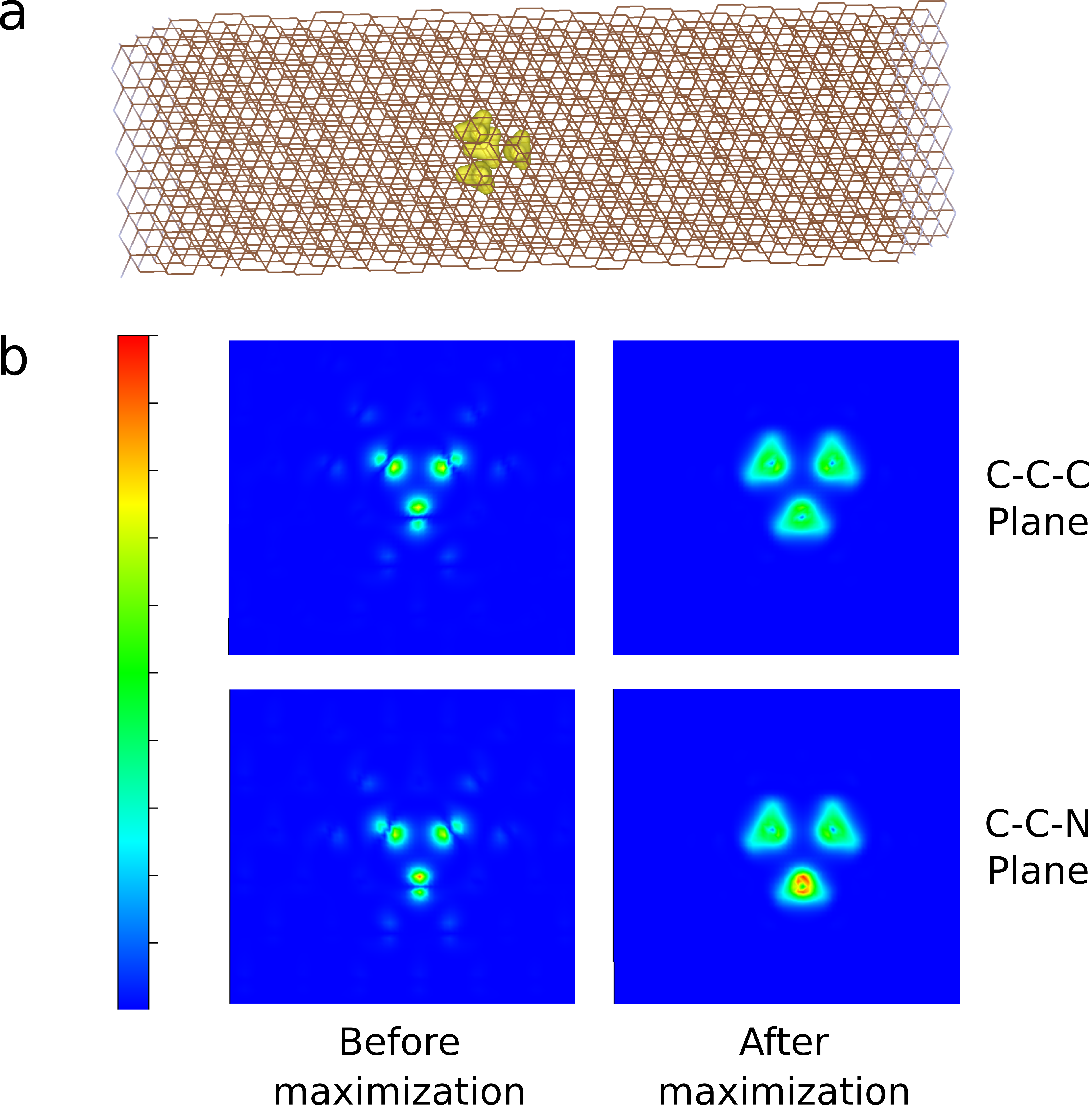
In the previous section, the completeness of sG-PMWF has been demonstrated for the maximization of the modified PM functional (Eq. 6). These 16 resulting states are localized on the fragment and serve as a subspace to further maximize the (Eq. 1), which unfolds the states on each individual atom. Table and summarize the converged and . The results of the sG-PMWF method differ from that of G-PMWF by no more than 0.0001 (). Figure to show that the electron density constructed from the 16 regionally localized states are visually identical between the sG-PMWF and G-PMWF calculations. The same agreement is also seen for the four selected individual “p-like” states (Figure to ). Figure 6a highlights the NV- center in the slab using the regionally localized electron density. The obtained electron density conserves the spatial symmetry across the C-C-C plane and the C-C-N plane (Figure 6b). The left panels of Figure 6b show the electron density constructed from the 16 most localized canonical states, while the right panels present the maximized results from the sG-PMWF calculation. It can be clearly seen that electron density distribution becomes much more concentrated on the selected atoms, indicating the effectiveness of the localization.
To demonstrate that the sG-PMWF localization is subsystem-independent, an arbitrary carbon atom is chosen from each investigated system, and four regionally localized states are sought. Figure shows that the electron density around the selected C atom is successfully reproduced for each system, confirming the generality of the sG-PMWF approach.
4.4.2 Excited states of the NV- center
To further demonstrate the practical application and quality of the sG-PMWF approach, we investigate the optical transitions in the NV- center using the “p”-like Wannier function basis (see Figure to ). To model the excited states of the NV- center, we solve the Hubbard Hamiltonian, defined in Eq. () in the SI. It is a minimal model of the NV- center that is commonly used Choi et al. 2012; Bockstedte et al. 2018; Ma et al. 2020; Ma et al. 2021 to describe its low-lying excited states. In this section, we will, in particular, comment on the selection of the fragment on which the electronic states are localized. Note that the fragment size is independent of the sG-PMWF methodology, but it represents an important parameter.
First, we focus on the results computed from the localized basis on the four-atom fragment (Figure a). The results for the three lowest energy transitions are in Table 1 in parentheses. For the 3D periodic systems, the – transition energy is slightly underestimated, while the – one is overestimated in the two small cells. For the bulk systems, the – and – transition energies are underestimated with respect to the experimental values of eV and eV, respectively. These results, however, are in good agreement with other theoretical calculations that employ PBE functionals to compute the bare Hubbard model parametersGoss et al. 1996; Gali et al. 2008; Delaney and Larsson 2010; Ma et al. 2010; Gordon et al. 2013; Alkauskas et al. 2014. The – transition energy fluctuates mildly with respect to the supercell size but maintains a comparable magnitude. The results computed from the sG-PMWF basis agree perfectly with the G-PMWF ones (see Table in the SI), confirming the equivalency of the two sets of localized orbitals.
Despite this, the slab results are strikingly different. Again, G-PMWF and sG-PMWF perfectly agree, but the transition energies are up to 70%-80% lower than those in the bulk. As we show below, this is due to the selection of the fragment size and independent of the completeness of the orbital space. To the best of our knowledge, we note that no calculations for shallow NV- centers in slabs have been done previously. Hence it is not possible to compare our results with any reference.
| Transition symmetry | Energy (eV) | |||
|---|---|---|---|---|
| 215-atom cell | 511-atom cell | 999-atom cell | slab | |
| – | 2.108 (1.560) | 2.277 (1.695) | 2.312 (1.710) | 1.343 (0.363) |
| – | 1.433 (1.325) | 1.310 (1.270) | 1.202 (1.193) | 1.159 (0.292) |
| – | 0.447 (0.378) | 0.435 (0.381) | 0.413 (0.368) | 0.329 (0.091) |
The slab results become more in line with bulk values if a larger fragment size is employed. The fragment studied in the previous sections is in fact a minimal model, i.e., the orbital localization is considered only on the 4 atoms where the “p”-likes states are located and, the total number of orbitals on these four atoms is 16. However, neglecting the neighboring atoms might lead to a mixed character of “p”-like states and C-C (or N-C) covalent bonds. To test this, we investigate four combinations of {,} fragments: for instance, {4,16} represents the case where 4 atoms are considered in maximizing (Eq. (6)) while 16 atoms (including the bonded atoms) are considered in maximizing (Eq. (8)). A detailed investigation of the various parameters is performed on the 215-atom system. The corresponding fragments are presented in Figure . The four Wannier functions used for the Hubbard model are illustrated in Figure .
Numerically, the {4,16} combination gives the closest solutions to the result computed using G-PMWF with localization on all atoms at once. We call these results “all-atom” calculations. Note that in this case, the optimization does not preferentially localize single-electron states near the defect; rather it seeks globally most localized states. Such an approach is not guaranteed to generate transformed PMW orbitals that are optimal for the mapping onto the Hubbard model. Indeed, we show this numerically below. For a better comparison, we also provide the spatial overlaps between the fragmentation approaches and the all-atom calculation, in Table .
In contrast, the results for the {4,4} combination represent the minimal fragment where the optimization is performed for sixteen orbitals on four atoms neighboring the defect center. These minimal PMWFs are showin in Figure and displays over-localization of the “p”-like states in the NV- center, i.e., the orbitals are less centered on the atoms and tend to merge at the geometric center. This is a purely numerical artifact of a too small optimization space which is alleviated (Figure ) when the 12 bonded atoms are included to compete with the geometric center for the electron density. Due to this, we disregard the {4,4} case further.
Upon visual inspection, the {16,16} combination graphically gives the most localized “p”-like orbitals (the third row in Figure ). To provide a quantitative measure of localization, we calculate the locality of each “p”-like state on the corresponding atom plus its neighboring bonded atoms to account for the environment
| (19) |
where denote the “p”-like state and sums over the four 4 atoms (1 atom + 3 bonded atoms). The value for each individual state is summarized in Table where we use the sum, , to represent the whole set of PMW functions. In agreement with the visual analysis, the {16,16} combination exhibits the strongest localization (Figure ) attributed to the modification of the objective functional (Eq. 6). As commented by JnssonJónsson et al. 2017 et al., the solutions to “maximally-localized Wannier functions” are actually not unique and sometimes ambiguous since the resulting localized orbitals are determined by the objective functionals. We emphasize that the traditional G-PMWF approach evaluates the overall orbital localization on all the atoms, but it does not necessarily reach maximal localization on a specific subsystem (fragment). Instead, the proposed fragmentation treatment in this work leads to an objective functional for regionally localized orbitals. We surmise that this approach is more beneficial for effective embedding and downfolding.
To further analyze the results, we use the four sets of PMW functions and compute the optical transition energies for the 215-atom system (Table 2). The {4,16} combination provides results that are closest to the all-atom calculations. We see that the – is the most sensitive to the basis while the other two are less. Compared with the most localized case ({16,16}), the other results are consistently underestimated by up to 0.55 eV. From these results, it is clear that the extent of orbital localization affects various observables differently. While some optical transitions for a given system are insensitive, others can be extremely dependent on the basis. The sensible strategy is to construct the maximal fragment that also provides the maximal localization on each atom of interest and seek convergence of the observables of interest.
| Transition symmetry | Energy (eV) | ||||
|---|---|---|---|---|---|
| {4,4} | {4,16} | {16,16} | {40,40} | all-atom | |
| – | 1.560 | 1.770 | 2.108 | 1.860 | 1.715 |
| – | 1.325 | 1.373 | 1.433 | 1.384 | 1.355 |
| – | 0.378 | 0.407 | 0.447 | 0.417 | 0.398 |
| 3.514 | 3.464 | 3.507 | 3.411 | 3.461 | |
In the rest of the paper, we employ the {16,16} fragment to obtain the PMW function basis and provide the detailed results in Tables . The excited-state transition energies are summarized in Table 1. For the bulk systems with the new “p”-like basis, – transition gap is enlarged by up to 0.6 eV from the less localized basis, while the other two transition energies are relatively less sensitive to the change of basis. These results again agree with various other theoretical calculations that employ PBE functionals to compute the bare Hubbard model parametersGoss et al. 1996; Gali et al. 2008; Delaney and Larsson 2010; Ma et al. 2010; Gordon et al. 2013; Alkauskas et al. 2014.
The effect of the fragment size is most pronounced for the slab. If the {16,16} fragment is used, the results are similar to those for the bulk systems. In detail: the – transition is predicted 1 eV lower than that in the bulk, while the other two are only slightly lower (by eV) compared to the 999-atom cell. Here, the significant lowering of the triplet-triplet transition energy in the slab can be attributed to the interplay with the surface states of N atom passivation layer. The surface states dive below the conduction band minimum of the bulk states and are located inside the band-gap and affect the position of the in-gap defect states. Finally, we remark that these observations underline the importance of fragment selection. However, they are completely independent of the proposed sG-PMWF methodology. Indeed, the results obtained with the sG-PMWF and G-PMWF methods are perfect (Table ) in each case, while the results depend on the fragment size.
5 Conclusions and Perspective
By introducing the fragmentation treatment and the sequential exhausting of the orbital space to the traditional G-PMWF method, we develop a swift, efficient, and robust algorithm, sG-PMWF, to obtain a set of regionally localized states on a subsystem of interest. The completeness and efficiency are insensitive to the choice of input parameters. The core idea is to reduce the dimensionality of matrices during the maximization process and leads to a reduced scaling from being hyper-quadratic to linear. For the applications of localized basis to the Hubbard model, the excited-state calculations are sensitive to the localized basis. While Pipek-Mezey scheme is an ideal candidate to provide localized states with optimal localization for the whole system, it does not necessarily leads to “maximally” localized orbitals on a specific subsystem. But in our fragmentation treatment, one can carefully select the atoms (the strategy is mentioned above) to reach “maximally” localized orbitals on the subsystem as well as avoiding the over-localization issue.
The resulting sG-PMWF method has five primary benefits: (1) largely shortens the time per SA iteration and makes it easier to monitor the progress of localization; (2) significantly lowers the total job time and scaling for systems with thousands of electrons; (3) provides regionally localized orbitals with higher extent of localization; (4) less demanding for computing resources, e.g., memory and CPUs; (5) can be performed without the knowledge of canonical eigenstates if it is coupled with stochastic methods (e.g., stochastic DFT). The stochastic basis search approach exhibits higher efficiency than the traditional method for systems with over 4000 electrons.
Furthermore, we want to comment on the following prospective applications of the sequential exhausting method: (1) this method can be generalized to obtain localized states of the whole system. Given that the rest space can always be updated or reconstructed by Gram-Schmidt orthogonalzaiton, the sG-PMWF calculation can then be sequentially applied to all the fragments in the whole system; (2) this method can be coupled with other maximizer, e.g., conjugated gradient and BFGS approach, to further facilitate the convergence of the PM functional.
We believe that the sG-PMWF method will find numerous applications in condensed matter problems, either in chemistry, materials science, or computational materials physics.
he Supporting Information provides additional texts, figures and tables listed below.
Texts: Downfolded effective Hamiltonian for the Hubbard Model; Excited states of the NV- center; Preparation of stochastic basis using deterministic eigenstates.
Figures: three fragments of different sizes and the all-atom system exemplied by the 215-atom cell; scaling of with respect to , evolution of the objective functional with respect to the outer-loop step using deterministic and stochastic basis, investigations of () on the 511-atom system, total wall time of orbital localization on the four investigated systems, relative number of SA iterations in the sG-PMWF calculations for 215- and 511-atom systems, scaling of time per iteration with respect to , electron density localized on the NV- center of the three solid systems, four “p-like” localized Wannier functions on the NV- center of the three solid systems, electron density localized on an arbitrary carbon atom of the four investigated systems, four “p-like” localized Wannier functions as well as the resulting electron density on the NV- center of the 215-atom system using different sizes of fragments;
Tables: transition energies obatined from different Wannier functions basis using energy-windowing truncated space, comparison of G-PMWF and sG-PMWF calculations with different and for the four investigated systems using the 4-atom fragment, comparison of the time spent on the folding and unfolding steps; time per outer-loop iteration and normalized time per outer-loop iteration in the sG-PMWF calculations of the four investigated systems, total wall time and normalized total wall time of G-PMWF and sG-PMWF calculations for the four investigated systems, time per steep-ascent step in the G-PMWF and sG-PMWF calculations, number of iterations required to reach convergence for the four investigated systems, converged maximized PM functional values, spatial overlap between the Wannier functions obtained from the fragment approaches with those obtained from the all-atom calculation, transition energies of the four investigated systems using the Wannier functions basis obtained from the G-PMWF calculations, comparison of G-PMWF and sG-PMWF calculations with different and for the four investigated systems using the 16-atom fragment.
References
- Wu et al. (2009) Wu, X.; Selloni, A.; Car, R. Phys. Rev. B 2009, 79, 085102.
- Gygi and Duchemin (2013) Gygi, F.; Duchemin, I. Journal of Chemical Theory and Computation 2013, 9, 582–587, PMID: 26589056.
- Miyake et al. (2009) Miyake, T.; Aryasetiawan, F.; Imada, M. Phys. Rev. B 2009, 80, 155134.
- Tomczak et al. (2009) Tomczak, J. M.; Miyake, T.; Sakuma, R.; Aryasetiawan, F. Phys. Rev. B 2009, 79, 235133.
- Choi et al. (2012) Choi, S.; Jain, M.; Louie, S. G. Phys. Rev. B 2012, 86, 041202.
- Weng and Vlček (2021) Weng, G.; Vlček, V. The Journal of Chemical Physics 2021, 155, 054104.
- Aryasetiawan et al. (2009) Aryasetiawan, F.; Tomczak, J. M.; Miyake, T.; Sakuma, R. Phys. Rev. Lett. 2009, 102, 176402.
- Pavarini et al. (2011) Pavarini, E.; Koch, E.; Vollhardt, D.; Lichtenstein (eds), A. The LDA+DMFT approach to strongly correlated materials; 2011.
- Bowler and Miyazaki (2012) Bowler, D. R.; Miyazaki, T. Reports on Progress in Physics 2012, 75, 036503.
- Lau et al. (2021) Lau, B. T. G.; Knizia, G.; Berkelbach, T. C. The Journal of Physical Chemistry Letters 2021, 12, 1104–1109, PMID: 33475362.
- Boys (1960) Boys, S. F. Rev. Mod. Phys. 1960, 32, 296–299.
- Foster and Boys (1960) Foster, J. M.; Boys, S. F. Rev. Mod. Phys. 1960, 32, 300–302.
- Marzari and Vanderbilt (1997) Marzari, N.; Vanderbilt, D. Phys. Rev. B 1997, 56, 12847–12865.
- Marzari et al. (2012) Marzari, N.; Mostofi, A. A.; Yates, J. R.; Souza, I.; Vanderbilt, D. Rev. Mod. Phys. 2012, 84, 1419–1475.
- Damle et al. (2015) Damle, A.; Lin, L.; Ying, L. Journal of Chemical Theory and Computation 2015, 11, 1463–1469, PMID: 26574357.
- Damle et al. (2017) Damle, A.; Lin, L.; Ying, L. Journal of Computational Physics 2017, 334, 1–15.
- Damle and Lin (2018) Damle, A.; Lin, L. Multiscale Modeling & Simulation 2018, 16, 1392–1410.
- Damle et al. (2019) Damle, A.; Levitt, A.; Lin, L. Multiscale Modeling & Simulation 2019, 17, 167–191.
- Vitale et al. (2020) Vitale, V.; Pizzi, G.; Marrazzo, A.; Yates, J. R.; Marzari, N.; Mostofi, A. A. npj Computational Materials 2020, 6, 66.
- Edmiston and Ruedenberg (1963) Edmiston, C.; Ruedenberg, K. Rev. Mod. Phys. 1963, 35, 457–464.
- Edmiston and Ruedenberg (1965) Edmiston, C.; Ruedenberg, K. The Journal of Chemical Physics 1965, 43, S97–S116.
- Löwdin (1966) Löwdin, P.-O. Quantum Theory of Atoms, Molecules, and the Solid State A Tribute to John C. Slater; 1966.
- von Niessen (1972) von Niessen, W. The Journal of Chemical Physics 1972, 56, 4290–4297.
- Pipek and Mezey (1989) Pipek, J.; Mezey, P. G. The Journal of Chemical Physics 1989, 90, 4916–4926.
- Jónsson et al. (2017) Jónsson, E. Ö.; Lehtola, S.; Puska, M.; Jónsson, H. Journal of Chemical Theory and Computation 2017, 13, 460–474.
- Clement et al. (2021) Clement, M. C.; Wang, X.; Valeev, E. F. Journal of Chemical Theory and Computation 2021, 17, 7406–7415, PMID: 34739235.
- Baer et al. (2013) Baer, R.; Neuhauser, D.; Rabani, E. Phys. Rev. Lett. 2013, 111, 106402.
- Cytter et al. (2018) Cytter, Y.; Rabani, E.; Neuhauser, D.; Baer, R. Phys. Rev. B 2018, 97, 115207.
- Chen et al. (2019) Chen, M.; Baer, R.; Neuhauser, D.; Rabani, E. The Journal of Chemical Physics 2019, 151, 114116.
- Fabian et al. (2019) Fabian, M. D.; Shpiro, B.; Rabani, E.; Neuhauser, D.; Baer, R. WIREs Computational Molecular Science 2019, 9, e1412.
- Nguyen et al. (2021) Nguyen, M.; Li, W.; Li, Y.; Rabani, E.; Baer, R.; Neuhauser, D. The Journal of Chemical Physics 2021, 155, 204105.
- Baer et al. (2022) Baer, R.; Neuhauser, D.; Rabani, E. Annual Review of Physical Chemistry 2022, 73, null, PMID: 35081326.
- Neuhauser et al. (2013) Neuhauser, D.; Rabani, E.; Baer, R. The Journal of Physical Chemistry Letters 2013, 4, 1172–1176.
- Romanova and Vlček (2022) Romanova, M.; Vlček, V. npj Computational Materials 2022, 8, 1–10.
- Neuhauser et al. (2013) Neuhauser, D.; Rabani, E.; Baer, R. Journal of Chemical Theory and Computation 2013, 9, 24–27.
- Ge et al. (2014) Ge, Q.; Gao, Y.; Baer, R.; Rabani, E.; Neuhauser, D. The Journal of Physical Chemistry Letters 2014, 5, 185–189.
- Neuhauser et al. (2017) Neuhauser, D.; Baer, R.; Zgid, D. Journal of Chemical Theory and Computation 2017, 13, 5396–5403.
- Dou et al. (2019) Dou, W.; Takeshita, T. Y.; Chen, M.; Baer, R.; Neuhauser, D.; Rabani, E. Journal of Chemical Theory and Computation 2019, 15, 6703–6711.
- Takeshita et al. (2019) Takeshita, T. Y.; Dou, W.; Smith, D. G. A.; de Jong, W. A.; Baer, R.; Neuhauser, D.; Rabani, E. The Journal of Chemical Physics 2019, 151, 044114.
- Neuhauser et al. (2014) Neuhauser, D.; Gao, Y.; Arntsen, C.; Karshenas, C.; Rabani, E.; Baer, R. Phys. Rev. Lett. 2014, 113, 076402.
- Vlček et al. (2017) Vlček, V.; Rabani, E.; Neuhauser, D.; Baer, R. J. Chem. Theory Comput. 2017, 13, 4997–5003.
- Vlček et al. (2018) Vlček, V.; Li, W.; Baer, R.; Rabani, E.; Neuhauser, D. Phys. Rev. B 2018, 98, 075107.
- Romanova and Vlček (2020) Romanova, M.; Vlček, V. J. Chem. Phys. 2020, 153, 134103.
- Vlcek (2019) Vlcek, V. J. Chem. Theory Comput. 2019, 15, 6254–6266.
- Zhang and Li (2014) Zhang, C.; Li, S. The Journal of Chemical Physics 2014, 141, 244106.
- Hirshfeld (1977) Hirshfeld, F. L. Theoretica chimica acta 1977, 44, 129–138.
- Cioslowski (1991) Cioslowski, J. Journal of Mathematical Chemistry 1991, 8, 169–178.
- Bader (1994) Bader, R. Atoms in Molecules: A Quantum Theory; International Ser. of Monogr. on Chem; Clarendon Press, 1994.
- Alcoba et al. (2006) Alcoba, D. R.; Lain, L.; Torre, A.; Bochicchio, R. C. Journal of Computational Chemistry 2006, 27, 596–608.
- Lillestolen and Wheatley (2008) Lillestolen, T. C.; Wheatley, R. J. Chem. Commun. 2008, 5909–5911.
- Lillestolen and Wheatley (2009) Lillestolen, T. C.; Wheatley, R. J. The Journal of Chemical Physics 2009, 131, 144101.
- Knizia (2013) Knizia, G. Journal of Chemical Theory and Computation 2013, 9, 4834–4843, PMID: 26583402.
- Janowski (2014) Janowski, T. Journal of Chemical Theory and Computation 2014, 10, 3085–3091, PMID: 26588279.
- Lehtola and Jónsson (2014) Lehtola, S.; Jónsson, H. Journal of Chemical Theory and Computation 2014, 10, 642–649.
- Knizia and Klein (2015) Knizia, G.; Klein, J. E. M. N. Angewandte Chemie International Edition 2015, 54, 5518–5522.
- Silvestrelli et al. (1998) Silvestrelli, P. L.; Marzari, N.; Vanderbilt, D.; Parrinello, M. Solid State Communications 1998, 107, 7–11.
- Silvestrelli (1999) Silvestrelli, P. L. Phys. Rev. B 1999, 59, 9703–9706.
- Thygesen et al. (2005) Thygesen, K. S.; Hansen, L. B.; Jacobsen, K. W. Phys. Rev. B 2005, 72, 125119.
- Giannozzi et al. (2017) others,, et al. J. Condens. Matter Phys. 2017, 29, 465901.
- Tkatchenko and Scheffler (2009) Tkatchenko, A.; Scheffler, M. Phys. Rev. Lett. 2009, 102, 073005.
- Otani and Sugino (2006) Otani, M.; Sugino, O. Phys. Rev. B 2006, 73, 115407.
- Troullier and Martins (1991) Troullier, N.; Martins, J. L. Phys. Rev. B 1991, 43, 1993.
- Perdew and Wang (1992) Perdew, J. P.; Wang, Y. Phys. Rev. B 1992, 45, 13244–13249.
- Choi et al. (2012) Choi, S.; Jain, M.; Louie, S. G. Physical Review B 2012, 86, 041202.
- Bockstedte et al. (2018) Bockstedte, M.; Schütz, F.; Garratt, T.; Ivády, V.; Gali, A. npj Quantum Materials 2018, 3, 1–6.
- Ma et al. (2020) Ma, H.; Govoni, M.; Galli, G. npj Computational Materials 2020, 6, 1–8.
- Ma et al. (2021) Ma, H.; Sheng, N.; Govoni, M.; Galli, G. Journal of Chemical Theory and Computation 2021, 17, 2116–2125.
- Goss et al. (1996) Goss, J. P.; Jones, R.; Breuer, S. J.; Briddon, P. R.; Öberg, S. Phys. Rev. Lett. 1996, 77.
- Gali et al. (2008) Gali, A.; Fyta, M.; Kaxiras, E. Phys. Rev. B 2008, 77.
- Delaney and Larsson (2010) Delaney, P.; Larsson, J. A. Phys. Procedia 2010, 3.
- Ma et al. (2010) Ma, Y.; Rohlfing, M.; Gali, A. Phys. Rev. B 2010, 81.
- Gordon et al. (2013) Gordon, L.; Weber, J. R.; Varley, J. B.; Janotti, A.; Awschalom, D. D.; Van De Walle, C. G. MRS Bull. 2013, 38.
- Alkauskas et al. (2014) Alkauskas, A.; Buckley, B. B.; Awschalom, D. D.; Van De Walle, C. G. New J. Phys. 2014, 16.