Effect of nonfactorizable background geometry on thermodynamics of clustering of galaxies

The clustering tendency of nebulae has been studied right from the 18th century with the cataloging of the observed objects by C. Messier and W. Herschel. At that time, the question that needed an answer was whether the nebulae were internal or external to the Milky Way. The answer came with Hubble’s work  1, wherein he proved that the concentrations seen were indeed systems like the Milky Way in their own right. Once the extra-galactic nature of nebulae was established, the galaxies were treated as physical systems by astronomers. In 1927, Lundmark  2 started the investigation on how the clusters form. Zwicky  3 was the first to estimate the mass of a cluster and proposed the mass discrepancy found in the clusters. In his work, Zwicky found that the mass should be greater by factors of 200–400 than the visible mass. He proposed that there is an invisible mass, which he called “dark matter”, in the clusters that has gravitational attraction but is otherwise non-detectable. Spitzer and Baade  4 proposed the collisional stripping theory, which leads to the study of clustering of galaxies as laboratories. These days, study of clustering of galaxies is very important astronomical laboratories on the largest scale, with a well characterized physical environment.

Multi-wavelength observational studies of galaxy clusters has provided tremendous information about the processes going on in the core of galaxy clusters. In recent past most of the information about the galaxy clusters has been obtained through X-ray spectroscopy. This is due to the high temperature (several KeV per particle) emission of the intracluster medium. Along with the spectroscopic observations much theoretical study has been made to understand and characterize this large-scale equilibrium structure. Theoretical models of clusters employ various techniques focused on the understanding of different properties of clusters. A simple model by Kaiser  5 which approximates cluster formation as dark matter driven dissipationless collapse of initial over-densities in an expanding universe. The predictions of this model are quite close to observations.

Saslaw and Hamilton in 1984  6 developed a new theory for clustering in an expanding universe. This model is based on thermodynamics of the gravitating systems and applies to nonlinear regime of clustering. This model predicts the distribution function of all orders from voids to thousands of galaxies. The main result of this theory is the probability distribution of finding $N$ galaxies in a volume $V$ of any shape given by

$$f(N)=e^{-\bar{N}(1-b)-Nb}\frac{\bar{N}(1-b)}{N!}\left[\bar{N}(1-b)+Nb\right]^{N-1},$$

(1)

where $\bar{N}=nV$ is the average number of particles expected in volume $V$ with average density $n$. The constant $b$ is the correlation parameter and can take values between $0$ and $1$. The applicability of thermodynamics to cosmological many-body problems paves way for the applicability of statistical mechanics. In this procedure analytical expressions for the partition function (grand canonical) is derived for the galaxies treated as point particles as well as for galaxies-with-halos (extended masses) 7. Recently, many modifications to general theory of relativity have been put forward 8. These models have implications for the evolution of density fluctuations in the early universe that has caused the large scale cosmic structure. For instance, $f(R)$ theory is one such candidate in which an additional term, a function $f(R)$ of Ricci curvature is added to Einstein-Hilbert action  9. These models give enhanced gravitational force on scales relevant to structure formation and hence an enhanced structure formation on these scales. There has also been progress in studying the effect of modified Newtonian potential on the clustering of galaxies 10; 10l; 11; 11a; 11b; 11c; 10a; 10b; 10c.

Conventionally we believe that Newton’s force law for gravity implies only four non-compact dimensions. This is also verified by the fact that the standard model matter cannot propagate in extra dimensions to a large distance without contradicting with the observations. This problem can be avoided if we confine standard model in a “$3$-brane” i.e. $3+1$-dimensional subspace. However, in case of gravity this model is not possible as gravity, being dynamics of spacetime itself, propagates in all dimensions. If we apply the above framework to gravity, the size of the extra dimensions should be sufficiently small (compactification) so that the model agrees with the current gravitational tests. These properties are a consequence of the fact that the metric of the four non-compact dimensions is independent of the coordinates in extra dimensions i.e. factorizable geometry. If we drop this assumption and take $4+n$ non-compact dimensions with a non-factorizable background geometry, the scenario changes significantly. Randall and Sundrum  12 in their work took $n=1$ ($u$-direction) i.e. $4+1$ non-compact dimensions and successfully reproduced an effective four dimensional theory of gravity with the potential given by

$$\phi(r)=G\frac{m^{2}}{r}\left(1+\frac{1}{r^{2}k^{2}}\right).$$

(2)

The leading term in equation (2) is the usual Newtonian potential and the second term is the correction generated due to Kaluza-Klein modes. This form of potential comes from the Randall–Sundrum geometry

$\displaystyle ds^{2}=a^{2}(u)\eta_{\mu\nu}dx^{\mu}dx^{\nu}-du^{2},$

(3)

where $\eta_{\mu\nu}$ is the four-dimensional Minkowski metric and $a(u)=e^{-k|u|}$ is the warp factor. This metric is nonfactorizable as this, unlike the usual Kaluza-Klein scenarios, can not be described by product of the four-dimensional Minkowski space and a (compact) manifold of extra dimensions.

Although galactic clustering under modified theories of gravity has been studied extensively, the study under the effect of nonfactorizable background geometry is not yet studied. This provides us an opportunity to bridge this gap. This is a motivation of present study. We present our study in the following manner. In section II, we construct the partition function for the system of galaxies. In section III, we quantitatively study the effect of the extra term ($r$ dependency) in Newton’s law on various thermodynamic equations of state, viz. free energy, entropy, and chemical potential, etc. We study the effects of this force form on the statistical distribution of galaxies in section IV. The behavior of specific heat as an indicator of possible phase transition is also studied in section V. The effect of the correction term yields a modified clustering parameter which estimates the extent of correlation among system particles. Finally we discuss the summary and future prospectus in the last section.

Here, in this section, we deduce the partition function of the system of galaxies treated as homogeneous over large regions in an expanding universe as has been previously done in Ref.  7. Our system consists of larger number of cells (ensemble of cells) with same volume $V$ or radius $R$ ($R<<V$), and have average number density $\bar{N}$. Also, we let the particle number and their total energy vary among the cells so that it represents the grand canonical ensemble. In this system the galaxies (particles) will interact only pairwise through gravitational force and over a large space or region the distribution of particles (galaxies) is statistically homogeneous.

The general form of the partition function of a system of $N$ galaxies of equal mass $m$ interacting gravitationally with a potential energy $\phi$ having average temperature $T$ and momenta $p_{i}$ is given by

$$Z_{N}(T,V)=\frac{1}{\lambda^{3N}N!}\int\exp{\left[-T^{-1}\left(\sum_{i=1}^{N}\frac{p_{i}^{2}}{2m}+\phi(r_{1},r_{2},...r_{N})\right)\right]}d^{3N}pd^{3N}r.$$

(4)

Here $N!$ takes care of distinguishability of classical system of particles and $\lambda$ is a normalization factor. Boltzmann’s constant is set unit here. Integrating over the momenta space, equation (4) simplifies to,

$$\hskip 56.9055ptZ_{N}(T,V)=\frac{1}{N!}\left(\frac{2\pi mT}{\lambda^{2}}\right)^{\frac{3N}{2}}Q_{N}(T,V),$$

(5)

where configurational integral

$$Q_{N}(T,V)=\displaystyle\int...\int\exp\left[-T^{-1}\phi(r_{1},r_{2},...r_{N})\right]d^{3N}r.$$

(6)

Generally, the gravitational potential energy function $\phi(r_{1},r_{2},...r_{N})$ is a function of the relative position vector $r_{ij}=|r_{i}-r_{j}|$ and is the sum of potential energy of all the pairs of particles. Here our main task is to evaluate the integral $Q_{N}(T,V)$. In our system of gravitating bodies the potential energy $\phi(r_{1},r_{2},...r_{N})$ of the system is due to all pairs of particles (galaxies) of which the system is made, i.e.

$$\phi(r_{1},r_{2},...r_{N})=\sum_{1\leq i\leq j\leq N}\phi(r_{i,j})=\sum_{1\leq i\leq j\leq N}\phi_{ij}(r).$$

(7)

With this simplification, equation (6) can now be written as

$$\hskip 56.9055ptQ_{N}(T,V)=\displaystyle\int...\int\displaystyle\prod_{1\leq i\leq j\leq N}\left[-T^{-1}\phi_{ij}(r)\right]d^{3N}r,$$

(8)

where $\phi_{ij}$ represents the potential energy due to gravitational interaction between the $i^{th}$ and $j^{th}$ particle. In order to solve the confugirational integral, we make use of the usual two-particle function defined as

$$f_{ij}=e^{-\frac{\phi_{ij}}{T}}-1.$$

(9)

The function $f_{ij}$ is identically zero if there is no interaction between the particles (galaxies) e,g ideal gases, and is non zero in presence of interaction. Also at extremely high temperature it is extremely small comparison with unity. With the substitution of two point function, $f_{ij}$, equation (8) takes the form

$$Q_{N}(T,V)=\int...\int\prod_{1\leq i\leq j\leq N}(1+f_{ij})d^{3}r_{1}d^{3}r_{2}...d^{3}r_{N}.$$

(10)

In the above integral, the higher order terms like $\sum f_{ij}f_{i}^{\prime}j^{\prime}$ can be dropped as these represent the interaction of more than two particles at once. However, in gravitating system all particles interact pairwise only, therefore the product in the equation (10) can be represented as

$$\displaystyle\prod_{1\leq i\leq j\leq N}(1+f_{ij})=\displaystyle\prod_{1\leq i}\prod_{i<j\leq N}{(1+f_{ij})}=\displaystyle\prod_{j=1,2,3,4...N}(1+f_{1j})(1+f_{2j})(1+f_{3j})...(1+f_{Nj}).$$

(11)

This sum excludes or neglects the terms involving self energy like $f_{jj}$. Hence when $j=2$ we have only one term $(1+f_{12})$. For $j=3$, we have just two terms $(1+f_{12})(1+f_{23})$ and so on.Therefore for other values of $j$ the above equation becomes

$$Q_{N}(T,V)=\displaystyle\int...\int(1+f_{12})(1+f_{13})(1+f_{23})(1+f_{14})...(1+f_{N-1,N})d^{3}r_{1}d^{3}r_{2}...d^{3}r_{N}.$$

(12)

Now, the main task remains the evaluation of this integral for various values of $N$ and then generalize it.

For point masses the particle function diverges when it includes energy states corresponding to $r_{ij}=0$, which in turn results in the divergence of Hamiltonian of the system. In order to remove this divergence we introduce a new parameter $\epsilon$, this $\epsilon$ is called the softening parameter. The typical value of softening parameter $\epsilon$ is $0.01\leq\epsilon\leq 0.05$ in units of the constant cell size 7. With the incorporation of softening parameter the modified Newtonian potential (2) can be written as

$$\phi_{ij}=Gm^{2}\left[\frac{1}{(r^{2}_{ij}+\epsilon^{2})^{1/2}}+\frac{1}{(r^{6}_{ij}+\epsilon^{6})^{1/2}k^{2}}\right].$$

(13)

Using this value of $\phi_{ij}$, we get the following two-particle function:

$$f_{ij}+1=e^{\frac{Gm^{2}}{(r^{2}_{ij}+\epsilon^{2})^{1/2}T}+\frac{Gm^{2}}{(r^{6}_{ij}+\epsilon^{6})^{1/2}Tk^{2}}}.$$

(14)

This can further be expanded to get,

$$\large f_{ij}=\frac{Gm^{2}}{T}\left[\frac{1}{(r^{2}_{ij}+\epsilon^{2})^{1/2}}+\frac{1}{(r^{6}_{ij}+\epsilon^{6})^{1/2}k^{2}}\right].$$

(15)

Since the system is not virialized on all scales, so the above expansion is dominating up to linear order only. Using equation (15) in equation (12), values of $Q_{N}$ for different values of $N$ can be obtained. For $N=1$, we have

$$Q_{1}(T,V)=V.$$

(16)

For $N=2$, first we fix the position of $r_{1}$ and evaluate the above integral over all the other particles. The integral simplifies to

$$Q_{2}(T,V)=V^{2}\bigg[1+Y(\beta_{1}+\beta_{2})\bigg],$$

(17)

where

$\beta_{1}=\sqrt{1+\frac{\epsilon^{2}}{R_{1}^{2}}}+\frac{\epsilon^{2}}{R_{1}^{2}}\log\frac{\epsilon/R_{1}}{1+\sqrt{1+\epsilon^{2}/R_{1}^{2}}},$

$\beta_{2}=\frac{1}{3R_{1}^{2}k^{2}}\log\bigg[\frac{1+\sqrt{1+\epsilon^{6}/R_{1}^{6}}}{\epsilon^{6}/R_{1}^{6}}\bigg],$

$Y=\frac{3Gm^{2}}{2TR_{1}}.$

Proceeding in the same way, the value of $Q_{N}$ for $N=3,4,5,...,N$ can be obtained. For $N=3$, we get

$$Q_{3}(T,V)=V^{3}\bigg[1+Y(\beta_{1}+\beta_{2})\bigg]^{2}.$$

(18)

Generalizing above equation for $N$ particles, we obtain

$$Q_{N}(T,V)=V^{N}\bigg[1+Y(\beta_{1}+\beta_{2})\bigg]^{N-1}.$$

(19)

Finally, substituting equation (19) into equation (4), we get the partition function for gravitating system of $N$ particles (galaxies) under the modified Newtonian potential as

$$Z_{N}(T,V)=\frac{1}{N!}\bigg(\frac{2\pi mT}{\Lambda^{2}}\bigg)^{\frac{3N}{2}}V^{N}\bigg[1+(\beta_{1}+\beta_{2})Y\bigg]^{N-1}.$$

(20)

This is the standard form of canonical partition function for a system of $N$ particles interacting through the modified Newton’s law. The modification due to the incorporation of nonfactorizable background geometry is inherent in the parameter $\beta_{2}$.

Once the partition function is known, it a matter of calculation to deduce various thermodynamic quantities. For example, the Helmholtz free energy for our system of galaxies can be obtained using the general statistical relation $F=-T\ln Z_{N}(T,V)$ along with equation (20). The free energy for the system of galaxies takes the following form:

$$F=NT\ln\bigg(\frac{N}{V}T^{\frac{-3}{2}}\bigg)-NT-\frac{3}{2}NT\ln\bigg(\frac{2\pi mT}{\lambda^{2}}\bigg)-NT\ln[1+Y(\beta_{1}+\beta_{2})].$$

(21)

Here, approximation $N-1\approx N$ is used. The effect of the correction term can also be depicted from the Fig. 1. Here, we see that correction term increases the value of free energy.

For a given free energy, we can study the other thermodynamic equations of state easily. The entropy of the system can be obtained using the fundamental relation, $S=-\bigg(\frac{\partial F}{\partial T}\bigg)_{V,N}$. For the Helmholtz free energy (21), the entropy of the system is calculated as

$$S=N\ln\biggl(\frac{V}{N}T^{3/2}\biggl)+N\ln[1+Y(\beta_{1}+\beta_{2})]-3N\frac{Y(\beta_{1}+\beta_{2})}{1+Y(\beta_{1}+\beta_{2})}+\frac{5}{2}N+\frac{3}{2}N\ln\bigg(\frac{2\pi m}{\lambda^{2}}\bigg).$$

(22)

The effect of the correction parameter $b^{*}Y$ on the entropy of the system of galaxies can be depicted from the graph (Fig. 2).

This equation can further be simplified to entropy per particle as

$$\frac{S}{N}=\ln\biggl(\frac{V}{N}T^{3/2}\biggl)-\ln[1-b^{*}]-3b^{*}+\frac{5}{2}+\frac{3}{2}\ln\frac{2\pi m}{\lambda^{2}},$$

(23)

where

$$b^{*}=\frac{\left(\beta_{1}+\beta_{2}\right)Y}{1+\left(\beta_{1}+\beta_{2}\right)Y},$$

(24)

is the modified clustering parameter that takes values between $0$ and $1$ and estimates the strength of correlation between system particles. The standard clustering parameter $b_{\epsilon}$, defined as $b_{\epsilon}=\frac{\beta_{1}Y}{1+\beta_{1}Y}$  7, is a limiting case of the modified parameter $b^{*}$ given in (24). These parameters are related as

$$b^{*}=\frac{b_{\epsilon}(1-\beta_{2}Y)+\beta_{2}Y}{1+\beta_{2}Y-b_{\epsilon}\beta_{2}Y}.$$

(25)

From the above relation, it is evident that $b^{*}\rightarrow b_{\epsilon}$ when $\beta_{2}\rightarrow 0$. The variation of the modified clustering parameter $b^{*}$ with the strength of the correction term can be visualized from the figure 3. The clustering becomes stronger as the value of the correction term increases. This, in turn, can affect the time-scale of clustering.

In order to study the internal energy of the system of galaxies, we use the basic definition of internal energy, $U=F+TS$. After substituting the calculated values of free energy (21) and entropy (22), this results

	$\displaystyle U$	$\displaystyle=$	$\displaystyle\frac{3}{2}NT\bigg[1-2\frac{Y(\beta_{1}+\beta_{2})}{1+Y(\beta_{1}+\beta_{2})}\bigg]$		(26)
		$\displaystyle=$	$\displaystyle\frac{3}{2}NT\left[1-2b^{*}\right].$

The graphical representation of the effect of the correction parameter on the internal energy of the system of galaxies can be seen in Fig. 4.

The pressure of the system can be calculated, using the fundamental definitions $P=-\bigg(\frac{\partial F}{\partial V}\bigg)_{T,N}$. Here, pressure is calculated as

	$\displaystyle P$	$\displaystyle=\frac{NT}{V}\left[1-\frac{Y(\beta_{1}+\beta_{2})}{1+Y(\beta_{1}+\beta_{2})}\right],$
		$\displaystyle=\frac{NT}{V}\left[1-b^{*}\right].$		(27)

The behavior of pressure of system with increasing particle number for different values of correction parameter $b^{*}Y$ can be visualized from the Fig. 5. Here, we clearly see that correction term decreases the entropy of the system.

The chemical potential of the system can be calculated using the relation $\mu=\bigg(\frac{\partial F}{\partial N}\bigg)_{T,V}$ as

	$\displaystyle\mu$	$\displaystyle=$	$\displaystyle T\bigg(\ln\frac{N}{V}T^{-\frac{3}{2}}\bigg)+T\ln\bigg[1-\frac{Y(\beta_{1}+\beta_{2})}{1+Y(\beta_{1}+\beta_{2})}\bigg]-T\frac{Y(\beta_{1}+\beta_{2})}{1+Y(\beta_{1}+\beta_{2})}-\frac{3}{2}T\ln\bigg(\frac{2\pi m}{\lambda^{2}}\bigg),$		(28)
		$\displaystyle=$	$\displaystyle T\left(\ln\frac{N}{V}T^{-3/2}\right)+T\ln\left[1-b^{*}\right]-Tb^{*}-\frac{3}{2}T\ln\left(\frac{2\pi M}{\lambda^{2}}\right).$

The figure 6 shows the graphical variation of the chemical potential $\mu$ with increasing particle number for different values of correction parameter $b^{*}Y$. The equations of state given in Eqs. (22), (26), (27) and (28) contain modified clustering parameter $b^{*}$ instead of $b_{\epsilon}$ as used in the original expressions 7.

The probability distribution function $f(N)$ characterizes the galactic clustering as it contains the voids distribution as well as the number of particles (galaxies) in cells of a given size distributed through out the system. The grand partition function is defined by

$$Z_{G}(T,V,z)=\sum_{N=0}^{\infty}\exp\left(\frac{N\mu}{T}Z_{N}(T,V)\right).$$

(29)

The distribution function of finding $N$ particles in a volume of a cell $V$ of grand canonical ensemble is given by

	$\displaystyle F(N)$	$\displaystyle=$	$\displaystyle\sum_{i=0}^{N}\frac{\exp\frac{N\mu}{T}\exp\frac{-U}{T}}{Z_{G}(T,V,z)},$		(30)
		$\displaystyle=$	$\displaystyle\frac{\exp\frac{N\mu}{T}Z_{N}(T,V)}{Z_{G}(T,V,z)}.$

Here, the weight factor $z=\exp\frac{\mu}{T}$ is the activity that represents the average value of $\bar{N}$. From this basic relation, we can calculate the distribution function. Exploiting the partition function (20) and the chemical potential (28), (30) the distribution function for the system of galaxies is given as

$$F(N)=\frac{\bar{N}}{N!}(1-b^{*})\bigg[\bar{N}(1-b^{*})+Nb^{*}\bigg]^{N-1}\exp-Nb^{*}-\bar{N}(1-b^{*}).$$

(31)

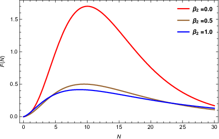
The basic structure of the distribution function is same as derived by Saslaw and Hamilton in Refs. 7; 13. The behavior of the distribution function as a function of particle number $N$ in two-dimensions is shown in figure 7. From the figure, it can be seen that the peak of the distribution function has flattened as the value of the correction parameter increases. We also infer that the correction parameter $\beta_{2}$ shifts the peak downwards without changing the basic structure of the curve.

The Poisson distribution (zero correlation) of a many-body system, driven gravitationally, evolves through many stages from zero correlation to some positive value of the correlation parameter $b^{*}$. This evolution can be characterized as a form of phase transition from uncorrelated phase to correlated phase, i.e., $b^{*}=0$ to $b^{*}>0$. Through this phase transition the homogeneity of the system is lost and lumps of particles are created. As an important indicator of phase transition, we analyze the variation of specific heat with temperature, $T$, of the system.

The specific heat (at constant volume) $C_{V}$ is defined as

$$C_{V}=\frac{1}{N}\left(\frac{\partial U}{\partial T}\right)_{V,N}.$$

(32)

For internal energy (26), the above equation leads to the specific heat of the system as

$$C_{V}=\frac{3}{2}\left[\frac{1+6\beta Y-4\beta^{2}Y^{2}}{\left(1+\beta Y\right)^{2}}\right],$$

(33)

where $\beta=\beta_{1}+\beta_{2}$. At $b^{*}=0$, the specific heat takes the value $C_{V}=3/2$. This corresponds to zero correlation of the system particles. At $b^{*}=1$, $C_{V}=-3/2$, which corresponds to fully virialized system. In between these two extreme values of the correlation parameter $b^{*}$, the specific heat takes an extreme value which corresponds to a phase transition within the system corresponding to a critical value of temperature, $T=T_{C}$, i.e.,

$$\frac{\partial C_{V}}{\partial T}\biggr\rvert_{T=T_{C}}=0.$$

In the modified potential the correlation parameter takes the value

$$T_{C}=\left[3\frac{\bar{N}}{V}\left(GM^{2}\right)^{3}\left(\beta_{1}+\beta_{2}\right)\right]^{1/3}.$$

(34)

The specific heat $C_{V}$ given in (33) can be expressed in terms of the above critical temperature as

$$C_{V}=\frac{3}{2}\left[1-2\frac{1-4\left(T/T_{C}\right)^{3}}{\left\{1+2\left(T/T_{C}\right)^{3}\right\}^{2}}\right].$$

(35)

At $T=T_{C}$, the specific heat becomes $C_{V}=5/2$, which is a property of a diatomic gas. This corresponds to the formation of binary systems and indicates the system symmetry breaking at average inter-particle separation. At this point the hierarchical phase transition occurs at the lowest scale and propagates to higher scales in the system. This behavior of specific heat is also evident from the Fig. 8 in which the specific heat varies finitely around critical temperature.

In this paper, we have analyzed the clustering of galaxies under a modified Newtonian potential motivated by the inclusion of nonfactorizable background geometry. Here, we have considered a strongly interacting system of galaxies and derived the gravitational partition function for galaxies interacting under the modified gravitational potential. We have also computed various thermodynamic equations of state for the system of galaxies. A general clustering parameter was also obtained for the system of galaxies. We observed that the correlation parameter gets stronger and stronger as the strength of the correction factor is increased. This behavior of the clustering parameter can affect the time scale of clustering of the galaxy systems. The effect of modification in the potential has also affected the distribution function of the system of galaxies. The corrected distribution function has a low peak as compared to the original distribution function. The evolution of the system with an increasing system temperature is characterized by the behavior specific heat implying a possibility of phase transition around the critical temperature.

References

- (1) Hubble, E. P. (1925). Cepheids in spiral nebulae. Popular Astronomy, 33.
- (2) Lundmark, K., Uppsala Mrdd.(1927). 30.
- (3) Zwicky, F. (1933). Die rotverschiebung von extragalaktischen nebeln. Helvetica physica acta, 6, 110-127.
- (4) Spitzer Jr, Lyman, and Walter Baade.(1951). Stellar Populations and Collisions of Galaxies. The Astrophysical Journal 113, 413.
- (5) Kaiser, N. (1986). Evolution and clustering of rich clusters. Monthly Notices of the Royal Astronomical Society, 222(2), 323-345.
- (6) Saslaw, W. C., and Hamilton, A. J. S. (1984). Thermodynamics and galaxy clustering-Nonlinear theory of high order correlations. The Astrophysical Journal, 276, 13-25.
- (7) Ahmad, F., Saslaw, W. C., and Bhat, N. I. (2002). Statistical mechanics of the cosmological many-body problem. The Astrophysical Journal, 571(2), 576.
- (8) Capozziello, S., and De Laurentis, M. (2011). Extended theories of gravity. Physics Reports 509.4-5, 167-321.
- (9) Jain, B., and Khoury, J. (2010). Cosmological tests of gravity. Annals of Physics, 325(7), 1479-1516.
- (10) Upadhyay, S. (2017). Thermodynamics and galactic clustering with a modified gravitational potential. Physical Review D, 95(4), 043008.
- (11) Hameeda, M., Pourhassan, B., Faizal, M., Masroor, C. P., Ansari, R.-Ul H., and Suresh, P. K. (2019). Modified theory of gravity and clustering of multi-component system of galaxies. The European Physical Journal C 79, 769.
- (12) Khanday, A. W., Upadhyay, S., and Ganai, P. A. (2021). Galactic clustering under power-law modified newtonian potential. General Relativity and Gravitation, 53(6), 1-19.
- (13) Upadhyay, S., Pourhassan, B., and Capozziello, S.(2019). Thermodynamics and phase transitions of galactic clustering in higher-order modified gravity. International Journal of Modern Physics D 28, 1950027.
- (14) Khanday, Abdul W., Upadhyay, S., and Ganai, P. A. (2021). Thermodynamics of galaxy clusters in modified Newtonian potential. Physica Scripta 96, 125030.
- (15) Hameeda, M., Upadhyay, S., Faizal, M., and Ali, A. F. (2016). Effects of cosmological constant on clustering of Galaxies. MNRAS 463, 3699-3704.
- (16) Hameeda, M., Upadhyay, S., Faizal, M., Ali, A. F., and Pourhassan, B. (2018). Large distance modification of Newtonian potential and structure formation in universe. Physics of the dark universe, 19, 137-143.
- (17) Pourhassan, B., Upadhyay, S., Hameeda, M., and Faizal, M. (2017). Clustering of galaxies with dynamical dark energy. MNRAS 468, 3166-3173.
- (18) Capozziello, S., Faizal, M., Hameeda, M., Pourhassan, B., Salzano, V., and Upadhyay, S. (2018). Clustering of galaxies with f(R) gravity. MNRAS 474, 2430-2443.
- (19) Randall, L., and Sundrum, R. (1999). An alternative to compactification. Physical Review Letters, 83(23), 4690.
- (20) Saslaw, W. C., and Hamilton, A. J. S. (1984). Thermodynamics and galaxy clustering-Nonlinear theory of high order correlations. The Astrophysical Journal, 276, 13-25.
- (21) Peebles, P. J. E. (2020). The large-scale structure of the universe (Vol. 98). Princeton university press.
- (22) Itoh, M., Inagaki, S., and Saslaw, W. C. (1993). Gravitational clustering of galaxies: Comparison between thermodynamic theory and N-body simulations. IV-The effects of continuous mass spectra. The Astrophysical Journal, 403, 476-496.