Statistical description of galaxy clusters in Finzi model of gravity
Abstract
We exploit a new theory of gravity proposed by Finzi, which gives stronger interaction at large scales, to study the thermodynamic description of galaxy clusters. We employ a statistical model to deduce various thermodynamics equations of state. In addition, we analyze the behavior of clustering parameter in comparison to its standard (Newtonian) counterpart. The general distribution function and its behavior with varying strength of clustering parameter are also studied. The possibility of phase transition is investigated and it is observed that a phase transition is possible though hierarchically. We also analyze the model by comparing the results with data available through SDSS-III, and obtain the parameters involved.
Keywords:
Finzi gravity; Distribution function of galaxies; Phase transition.I Introduction
The distribution of matter on large scale is mainly described by the gravitational interaction. It is believed that the large scale structure of the universe is a gravitationally amplified descendant of a faint noise field believed to be seeded by quantum fluctuations in the early universe. A linear theory for initial perturbations to the present observed matter distribution has been developed extensively 1. The formation of first structures in the universe took place at a red-shift of in the dark matter halos of masses, 2. This structure formation took place on the imprints of small matter density perturbations in the primordial matter density field. It has been verified by -body simulations that the initial density perturbations have the potential to grow to the scale of present day observed structure 3.
It is well-known that the peculiar velocity of galaxies in a cluster doesn’t agree well with the total mass of the visible matter. The estimated mass was times less than the mass required to prevent the rupture of the galaxies from the cluster 4. This led to the concept of dark matter. There is a strong support to the dark matter hypothesis, but the identification of the particles that compose this matter is yet under discussion. One explanation to this could be a strong correlation between the dark matter and baryonic matter 5. The other intriguing idea could be a relevance of modified Newtonian dynamics (MoND) or any new dynamics on galactic scales.
The formation and distribution of galaxy clusters are crucial to understand the evolution of the structure formation in the universe. Saslaw and Hamilton developed a thermodynamic model for nonlinear regime of the clustering of galaxies in an expanding universe 7. The theoretical predictions of this model involve the distribution of voids as well as galaxies corresponding to under-dense and over-dense regions, respectively, in the initial density field. The probability distribution function of galaxies found in some volume predicted by this theory is given by
| (1) |
where is the ensemble-average of particles found in any volume and is clustering parameter.
It is well known that the force accounting for the flat rotation curve of galaxies and galaxy clusters requires stronger gravity at very larger spatial distances than produced by Newton’s law of gravity. Recently, there have been several attempts to account for this discrepancy through the modification to the general theory of relativity 8 . For instance, in group of theories, a function of Ricci scalar is used in place of Ricci scalar to account for the enhanced gravitational interaction on large scales. The force field that governs the large scale structure formation also governs the distribution of mass at this scale. We can employ statistical methods to find the statistical distribution of matter at largest possible scales 9. Recently there has been a lot of progress on the study of the effect of modified gravity laws on the clustering of galaxies using statistical mechanics 10; 11; 12; 13; 14; 15; 15a; 15b; 16; 17; 18; 19. The effect of the modifications incorporated has been anticipated in the strength of the clustering parameter . For instance, in 14, the modification to the clustering parameter as a function of correction factor has been studied.
In 1963, Finzi proposed a law of gravitation that gives a stronger interaction at relatively larger distances than predicted by Newton’s law of gravity 20. This force form can explain the larger velocities of galaxies in clusters without involving the concept of dark matter. The potential energy function proposed by Finzi is given by
| (2) |
where , is a constant (equivalent to gravitational constant ) and is a characteristic length beyond which the potential becomes significant. This potential reduces to the usual Newtonian potential at distances . The correlation and distribution function of galactic clusters has not been studied for Finzi approximation. Here, we try to bridge this gap and also make a comparison of the effect of this model to the already studied theories.
Our investigations are presented systematically as following. We construct the general partition function under Finzi potential for our system of galaxies in section II. Here, in order to avoid divergence, we consider extended nature of galaxies. We derive the various thermodynamic potentials along with their behavior under different circumstances, e.g., Helmholtz free energy, pressure, internal energy, entropy and chemical potential in section III. In section IV, we compare the clustering parameters with increasing radial distance corresponding to Newtonian and Finzi gravity. In section V, we study the statistical distribution of galaxies in the new gravity law.The power-law behavior for the correlation function is presented in section VI. Finally we investigate the possibility of phase transition in section VII. We present the results and their importance in the last section.
II The partition function
In this section, we develop the general partition function by taking into consideration a system of gravitationally interacting particles, with the interaction defined by Finzi gravity. We assume the clustering of galaxies in the expanding background to be in quasi-equilibrium state forming an ensemble of co-moving cells. We assume the system consists of an ensemble of cells of equal volume with number density . The form of the partition function for such a system of pairwise interacting particles having correlation energy and average temperature is given by 9
| (3) |
Here, is the normalization constant and the factor takes into account the distinguishability of the system particles. The Boltzmann’s constant,, is set equal to unity. Configuration part of the equation (3) can be written as
| (4) |
The gravitational potential energy function is a function of the relative positions and is summed over all the pairs of particles. In the system of gravitationally interacting bodies, the potential energy is due to all pairs of particles present in the system, i.e.
| (5) |
With this simplification (5), equation (4) can now be written as
| (6) |
where is the two point interaction energy between the and particle. The configuration integral can be written in terms of two-point function defined as:
| (7) |
Here, we note that the two-point function is non-zero only when there are interactions present. The Finzi potential (2) diverges for the point-particle nature of galaxies. Therefore, we need to express potential (2) by considering the extended nature of galaxies (galaxies with halos). This is done by introducing the softening parameter in the potential as
| (8) |
By substituting the two-point function corresponding to potential (8) in equation (7), the value of for various values of can be easily calculated. For instance, for , we have
| (9) |
For value, we evaluate the integral (Eqn. 7) by fixing the position of and integrating over all the other system particles. This simplifies the integral to
where and .
Proceeding in similar fashion , the values of for can be easily calculated. For , we get
| (10) |
In general the above equation, Eqn.(10), for number of particles takes the form,
| (11) |
Finally, substituting equation (11) into equation (3), we obtain the general partition function for an interacting system of particles (galaxies) as
| (12) |
Equation (12) is the standard partition function (Canonical) of the system of particles interacting through the modified gravity law (2). The correction to the partition function is inherent in the parameter .
III Thermodynamic equations of state of the system
The partition function equation (12) contains all the necessary information about the macroscopic variable (free energy, entropy, internal energy, pressure, chemical potential ) of the system. The Helmholtz free energy for the system of galaxies can be deduced from the partition function via the relation . For our system of galaxies the free energy takes the following form:
| (13) |
Here, we approximated . In equation (13), the parameter is defined as
| (14) |
This is the modified clustering parameter which contains information of the strength of correlation that governs the time evolution of the galaxy cluster and can take values between and .

Once the free energy is known, other thermodynamic equations of state can be estimated easily. For example, we can calculate the entropy of the system of galaxies utilizing the relation, . Substituting equation(13) in this relation the entropy of the system takes the following form:
| (15) |
Specific entropy i.e., entropy per particle of the system corresponding to equation (13) takes the following form
| (16) |

The total internal energy of the interacting system of galaxies can be calculated using the basic definition, . Upon substituting the values for free energy () (13) and entropy () (14), the relation for internal energy of the system in terms of the new clustering parameter takes the form
| (17) | |||||

Figure (3) shows the graphical visualization of the effect of modified clustering parameter on the internal energy function of the system of galaxies interacting gravitationally.
The equation of the pressure caused by the particles in the system can be obtained utilizing the fundamental relations . Using relation (13), the pressure of the system takes the form:
| (18) |

Finally, we deduce the relation for the chemical potential of the system using the fundamental relation, as
| (19) | |||||
The graphical visualization of the variation in the chemical potential of the system with an increase in the particle number can be seen in figure (5)

IV A Comparison of New and old clustering parameter
In this section the clustering parameter developed in this work based on the Finzi model of gravity is compared with the standard parameter defined in 9. The correlation parameter gives the strength of correlation and will in turn decide the time-length of clustering.
From the graph (Fig.(6)) it can been seen that the new clustering parameter is more strong than the standard one. This is due to the effect of the increased strength of the potential energy function at large distances as defined in the Finzi model.
V General form of the distribution function
The general form of the distribution function , which characterizes the galaxy clustering, describes the distribution of voids as well as the number of galaxies in fixed volume cells distributed through out the system. Here we let the system particles cross the cell boundaries which in turn can change the particle number in each cell. Thus we derive the grand canonical partition function defined as
| (20) |
The probability distribution function of particles contained in cells of fixed volume in a grand canonical ensemble is given by
| (21) | |||||
The factor is the fugacity of the system and it determines the activity within the system. From this basic equation (21), the general form of the distribution function of system can be determined easily. Utilizing the partition function (20) with chemical potential equation (12) the distribution function of the system takes the following form:
| (22) |
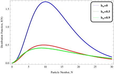
From equation (22) we confirm that there is no change in the basic structure of the distribution function in Finzi gravity model to the one derived by Saslaw and Hamilton for Newtonian gravity 7; 13. The graphical representation of the probability distribution function with increasing particle number is shown in figure 7. From the figure, it is clearly visible that the peak value in the distribution function decreases with an increase in the value of the clustering parameter.
VI Power law for two-point correlation function
Here we study the behavior of the two-point correlation function in the new model of gravity. We write the clustering parameter in the form 21
| (23) |
where is the number density and is the two-point correlation function.
Using the relation and equation (24), we obtain the following expression for the power law
| (25) |
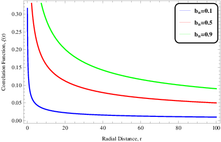
The graphical representation of the two point correlation function can be visualized from the figure (8). We can see the strength of the correlation function decreases with increasing radius. This leads us to an important result about the correlation of system points in different cells.The galaxies within a cell are more correlated than the galaxies in the adjacent cells. Thus the transfer of system points from cell to cell are less likely although not negligible.
VII Possibility of phase transition
If an interaction is introduced in a system characterized by Poisson distribution the system has a high chance of changing phase from less correlated to highly correlated. The possibility of phase transition in case of our system of galaxies interacting gravitationally can not be ignored. Here we will try to find out if the Finzi interaction can cause a phase transition in the system of gravitationally interacting point particles. The result is important as the possible phase transition can break the homogeneity of the system and cause lumpiness in the structure. Among many indicators of phase transition, specific heat is an important candidate to track.
The specific heat (at constant volume) is defined as
| (26) |
Using the relation for internal energy (17), the specific heat of the system takes the following form
| (27) |
As , this corresponds to no interaction among the system particles. As , which means the system is fully virialized. Between these two extreme values lie the maximum values of specific heat at some critical value of temperature. This extreme value of specific heat indicates a possible phase transition at .
This gives an expression for the critical temperature as
| (28) |
In terms of critical temperature the specific heat of the system, , given in (27) can be written as
| (29) |
At , a property of a diatomic gas. This is an indication of system symmetry breaking due to the formation of binaries. The phase transition is hierarchical and not spontaneous as observed in many other physical systems. The graphical behavior of the specific heat is visualized in figure (9).

VIII observational data
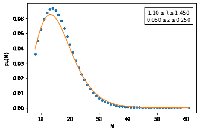
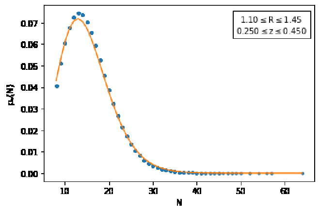
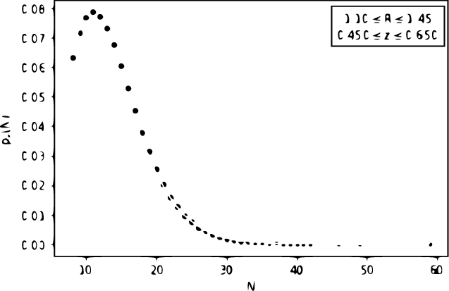
In this section we test our model with the data obtained through Sloan Digital Sky Survey III (SDSS-III) through its newest Data Release (DR12). SDSS-III contains additional sky coverage and better galaxy estimates than SDSS-I and SDSS-II. The data is present in catalog 22. In figure (11) the sky distribution of galaxy clusters in various RA and DEC coordinates is presented from this catalog. This catalog contains an information (RA, DEC, z, N etc) of almost 132,684 clusters. The catalog gives a parameter which is the distance up to which mean density is 200 and also the number of galaxy clusters in it i,e . Figure (10,(a)-(i)) shows the model fitted to the data.
First we bin the data on the basis of radius and Redshift . The bin size is chosen to be and . We divide cells by physical boundaries i.e., . The probability distribution of each cluster is determined by substituting arbitrary values for the fitting parameter and . The model is then fit through Application Programming Interface (API) Scipy.optimize.curve_fit of SciPy python Library. We obtained the optimized values for the parameters involved in equation(22), listed in table(1).
The value of the charaecteristic length, , is obtained through the relation,
| (30) |
We have set all other parameters to unity in (30). The characteristic length is measured in the same units as . For instance, the value means for 1 unit of , the characteristic length is 5 units.
![[Uncaptioned image]](2203.17237v4/plot_1.png)
![[Uncaptioned image]](2203.17237v4/plot_2.png)
![[Uncaptioned image]](2203.17237v4/plot_3.png)
![[Uncaptioned image]](2203.17237v4/plot_4.png)
![[Uncaptioned image]](2203.17237v4/plot_5.png)
![[Uncaptioned image]](2203.17237v4/plot_6.png)
![[Uncaptioned image]](2203.17237v4/ra_1.png)
![[Uncaptioned image]](2203.17237v4/ra_2.png)
![[Uncaptioned image]](2203.17237v4/ra_3.png)
![[Uncaptioned image]](2203.17237v4/ra_4.png)
![[Uncaptioned image]](2203.17237v4/ra_5.png)
![[Uncaptioned image]](2203.17237v4/ra_6.png)


IX Conclusion
The velocities of galaxies in a cluster are much higher than depicted by the visible matter which brings in the concept of gravitating non-visible matter called dark matter. While the hunt for the exact description is underway, it is plausible to reconsider Newtonian dynamics and modify it to fit the observed data.
In this work, we have considered a gravitational potential proposed by Finzi and, by using statistical methods, we deduced various thermodynamic quantities along with correlation function. A graphical analysis of various thermodynamic equations of state was also done. A new clustering parameter was deduced based on this theory which shows a greater strength as compared to the standard one. We have also made a graphical comparison of the the clustering parameters for Finzi and Newtonian gravity. From the behavior of the clustering parameter, it is obvious that the Finzi model of gravity at larger scale is more significant. The power-law of the correlation function for Finzi model is also discussed. We also studied possibility of phase transition within the system. The comparison of our results with the data was also studied and it could be seen that the model fits the data very closely in some Redshift and radius ranges , while in some regions the fit is not too appropriate although there is agreement with the trend.
References
- (1) Lifshitz, E. (2017). Republication of: On the gravitational stability of the expanding universe. General Relativity and Gravitation, 49(2), 1-20.
- (2) Bromm, V., Yoshida, N., Hernquist, L., and McKee, C. F. (2009). The formation of the first stars and galaxies. Nature, 459(7243), 49-54.
- (3) Klypin, A. A., and Shandarin, S. F. (1983). Three-dimensional numerical model of the formation of large-scale structure in the Universe. Monthly Notices of the Royal Astronomical Society, 204(3), 891-907.
- (4) Zwicky, F. (1933). Die rotverschiebung von extragalaktischen nebeln. Helvetica physica acta, 6, 110-127.
- (5) McGaugh, S., Lelli, F., and Schombert, J. (2016). The Radial Acceleration Relation in Rotationally Supported Galaxies, eprint. arXiv preprint arXiv:1609.05917.
- (6) Saslaw, W. C., and Hamilton, A. J. S. (1984). Thermodynamics and galaxy clustering-Nonlinear theory of high order correlations. The Astrophysical Journal, 276, 13-25.
- (7) Capozziello, S., and De Laurentis, M. (2011). Extended theories of gravity. Physics Reports 509.4-5, 167-321.
- (8) Ahmad, F., Saslaw, W. C., and Bhat, N. I. (2002). Statistical mechanics of the cosmological many-body problem. The Astrophysical Journal, 571(2), 576.
- (9) Upadhyay, S. (2017). Thermodynamics and galactic clustering with a modified gravitational potential. Physical Review D, 95(4), 043008.
- (10) Hameeda, M., Pourhassan, B., Faizal, M., Masroor, C. P., Ansari, R.-Ul H., and Suresh, P. K.(2019). Modified theory of gravity and clustering of multi-component system of galaxies. The European Physical Journal C 79, 769.
- (11) Khanday, A. W., Upadhyay, S., and Ganai, P. A. (2021). Galactic clustering under power-law modified newtonian potential. General Relativity and Gravitation, 53(6), 1-19.
- (12) Upadhyay, S., Pourhassan, B., and Capozziello, S.(2019). Thermodynamics and phase transitions of galactic clustering in higher-order modified gravity. International Journal of Modern Physics D 28, 1950027.
- (13) Khanday, Abdul W., Upadhyay, S., and Ganai, P. A. (2021). Thermodynamics of galaxy clusters in modified Newtonian potential. Physica Scripta 96, 125030.
- (14) Hameeda, M., Upadhyay, S., Faizal, M., and Ali, A. F. (2016). Effects of cosmological constant on clustering of Galaxies. MNRAS 463, 3699-3704.
- (15) Khanday, Abdul W., Upadhyay, S., Bagat, Hilal, A. and Ganai, P. A.(2022).Effect of nonfactorizable background geometry on the thermodynamics of galaxy clusters. MPLA, 37, 2250111.
- (16) Qadri, D. A., Khanday, A. W., and Ganai, P. A. (2022). A simplistic approach to the study of two-point correlation function in galaxy clusters. arXiv preprint arXiv:2206.15173.
- (17) Hameeda, M., Upadhyay, S., Faizal, M., Ali, A. F., and Pourhassan, B. (2018). Large distance modification of Newtonian potential and structure formation in universe. Physics of the dark universe, 19, 137-143.
- (18) Pourhassan, B., Upadhyay, S., Hameeda, M., and Faizal, M. (2017). Clustering of galaxies with dynamical dark energy. MNRAS 468, 3166-3173.
- (19) Capozziello, S., Faizal, M., Hameeda, M., Pourhassan, B., Salzano, V., and Upadhyay, S. (2018). Clustering of galaxies with f(R) gravity. MNRAS 474, 2430-2443.
- (20) Randall, L., and Sundrum, R. (1999). An alternative to compactification. Physical Review Letters, 83(23), 4690.
- (21) Finzi, A., and Pirani, F. A. E. (1963). On the validity of Newton’s law at a long distance. Monthly Notices of the Royal Astronomical Society, 127(1), 21-30.
- (22) Iqbal, N., Ahmad, F., and Khan, M. S. (2006). Gravitational clustering of galaxies in an expanding universe. Journal of Astrophysics and Astronomy, 27(4), 373-379.
- (23) Wen, Z. L., J. L. Han, and F. S. Liu. ”A catalog of 132,684 clusters of galaxies identified from Sloan Digital Sky Survey III.” The Astrophysical Journal Supplement Series 199.2 (2012): 34.