Hybrid discrete-continuous truncated Wigner approximation
for driven, dissipative spin systems

The density operator $\hat{\rho}$ of a quantum system with continuous degrees of freedom can equivalently be represented by the Wigner function. For example, a quantum particle with position $\hat{q}$ and momentum $\hat{p}$ has a corresponding quasiprobability distribution $W(q,p)$ of continuous scalars $q,p$. The connection between the Hilbert space and Wigner phase space is given by

where

are continuous phase-point operators Wigner 1932; Fano 1957; Hillery et al. 1984. Expectation values of any observable $\hat{O}$ can then be calculated by taking the statistical average of the corresponding Weyl symbol $\mathcal{O}$ with respect to the Wigner function

over the whole phase space, where the Weyl symbol ${\cal O}$ is defined via

The concept of phase space representations can be extended to quantum systems with a finite-dimensional Hilbert space Wootters 1987 such as spin-$\frac{1}{2}$ systems. To this end, Wootters Wootters 1987 introduced four discrete phase-point operators

where $\hat{\bm{\sigma}}=(\hat{\sigma}^{x},\hat{\sigma}^{y},\hat{\sigma}^{z})^{T}$ is the vector of Pauli matrices, $\bm{\alpha}=(\alpha_{1},\alpha_{2})$ with elements $\alpha_{i}\in\{0,1\}$ and the vector $\bm{r}_{\bm{\alpha}}$ is given by the discrete set of points

on the sphere with radius $r=\sqrt{3}$. The phase-point operators have unit trace $\text{Tr}(\hat{A}_{\bm{\alpha}})=1$, are orthogonal $\frac{1}{2}\text{Tr}(\hat{A}_{\bm{\alpha}}\hat{A}_{\bm{\beta}})=\delta_{\bm{\alpha}\bm{\beta}}$, and form a basis. The density operator $\hat{\rho}$ can then be expanded as

where the weights $W_{\bm{\alpha}}=\frac{1}{2}\text{Tr}[\hat{A}_{\bm{\alpha}}\hat{\rho}]$ are called the discrete Wigner function and are real by construction.

Note that since $r=\sqrt{3}>1$, the phase-point operators $\hat{A}_{\bm{\alpha}}$ are not positive definite and therefore are not density matrices themselves. As a consequence, the discrete Wigner function $W_{\bm{\alpha}}$ is in general not positive, but is normalized $\text{Tr}\,\hat{\rho}=\sum_{\bm{\alpha}}W_{\bm{\alpha}}=1$. Just as in the continuous case, the Wigner function represents only a quasi-probability distribution, therefore preventing a stochastic (Monte Carlo) sampling of arbitrary states. But for certain relevant quantum states, all Wigner coefficients are positive and can therefore be interpreted as proper probabilities. For example, the fully-polarized spin states

can be represented as equally weighted classical mixtures of $\hat{A}_{00}$ and $\hat{A}_{01}$ (for $|\!\uparrow\rangle\langle\uparrow\!|$), and $\hat{A}_{10}$ and $\hat{A}_{11}$ (for $|\!\downarrow\rangle\langle\downarrow\!|$).

It follows from the von Neumann equation $\frac{d}{dt}\hat{\rho}(t)=-i[\hat{H}_{0},\hat{\rho}(t)]$ ($\hbar=1$) for the unitary time evolution under some single-particle Hamiltonian $\hat{H}_{0}$ that the evolution equations for the phase-point operators are

Note that these equations describe the time evolution in the Schrödinger picture, as the phase point operators correspond to the quantum state. Since each of the four phase-point operators $\hat{A}_{\bm{\alpha}}$ is a linear combination of the Pauli spin matrices $\hat{\sigma}^{x},\hat{\sigma}^{y},\hat{\sigma}^{z}$, their time evolution can be expressed in terms of a time-dependent vector $\bm{s}_{\bm{\alpha}}(t)=\Bigl(s^{x}_{\bm{\alpha}}(t),s^{y}_{\bm{\alpha}}(t),s^{z}_{\bm{\alpha}}(t)\Bigr)$,

Here $s^{\mu}(t)$ ($\mu=x,y,z$) obey the equations of motion for a classical spin (see Appendix A),

where the classical Hamiltonian ${\cal H}_{0}({\bm{s}})$ is the Weyl symbol corresponding to $\hat{H}_{0}$ and we have dropped the index $\bm{\alpha}$ for notational simplicity. The initial conditions of the vector $\bm{s}_{\bm{\alpha}}$ are: $\bm{s}_{\bm{\alpha}}(t=0)=\bm{r}_{\bm{\alpha}}$. Evaluating the expectation value of any observable $\langle\hat{O}(\hat{\bm{\sigma}}(t))\rangle$ then amounts to calculating the time evolution of the Weyl symbol ${\cal O}({\bm{s}}(t))=\textrm{Tr}\left\{\hat{O}\hat{A}_{\bm{\alpha}}(t)\right\}$ averaged over the initial discrete Wigner distribution

If the initial state $\hat{\rho}(0)$ has positive Wigner coefficients $W_{\bm{\alpha}}$, as for the state $|\negmedspace\uparrow\rangle$ or $|\negmedspace\downarrow\rangle$ in Eqs. (7), Eq. (11) can be evaluated as a classical average of the Weyl symbols weighted by the initial probabilities $W_{\bm{\alpha}}(0)$. The ”quantumness” of the spin is then captured by the averaging over the initial conditions. This is possible without further approximation since we consider a single spin-$\frac{1}{2}$ particle without interactions and decay, in which case the Heisenberg equations of motion are also linear.

The utility of the discrete phase-space approach stems from its application to many interacting spins, which in general have complicated and intractable many-body dynamics. The phase space representation is the basis of the DTWA Schachenmayer et al. 2015, allowing it to take lowest-order quantum fluctuations into account and thus going beyond the mean-field level. Below, we outline the essence of the DTWA.

The density matrix for $N$ interacting spins can be faithfully represented by $4^{N}$ discrete Wigner coefficients and the corresponding phase point operators

As for a single spin, the dynamics of $\hat{\rho}$ can then be mapped onto the dynamics of the $4^{N}$ phase point operators $\hat{A}_{\bm{\alpha}_{1},\dots,\bm{\alpha}_{N}}(t)$, whose general evaluation in time requires exponentially increasing effort in $N$. The key approximation in the DTWA that makes the many-body problem tractable is the factorization of the phase point operators at all times:

The many-body density operator at time $t$ is then explicitly given by

which, for a factorized initial state, is further simplified to $W_{\bm{\alpha}_{1},\dots,\bm{\alpha}_{N}}(0)=\prod_{n}W_{\bm{\alpha}_{n}}(0)$.

Substituting the factorization ansatz of Eq. (13) into the equation of motion with a many-body Hamiltonian $\hat{H}$,

and using the orthogonality of the phase point operators, one finds that the time evolution of the single-spin operators is governed by

Here the mean-field Hamiltonian $\hat{H}_{j}^{\textrm{MF}}$ for $j$th spin is obtained by replacing all the other spin operators $\hat{\bm{\sigma}}_{l}$ by the corresponding c-numbers $\bm{s}_{l}^{\bm{\alpha}}(t)$. Using the decomposition of the phase point operators in Eq. (9), we thus find that $s_{j}^{\mu}(t)$ $(\mu=x,y,z)$ obey the classical equations of motion with the classical many-body Hamiltonian,

with initial conditions $\bm{s}_{j,\bm{\alpha}_{j}}(t=0)=\bm{r_{j,\bm{\alpha}_{j}}}$. As in the case of a single spin, all quantum mechanical observables are obtained from the solutions of the classical (mean-field) equations (17) and averaging over the initial Wigner distribution

It is worth noting that, despite the mean-field character of the DTWA, the quantum nature of the problem is taken into account to some extent in two ways. Firstly, as in the case of a single spin, the averaging over the initial conditions for every spin captures lowest-order quantum fluctuations on the single-particle level. Secondly, information about initial (quantum) correlations between the spins is, in principle, contained in $W_{\bm{\alpha}_{1},\dots,\bm{\alpha}_{N}}(0)$. Hence, the DTWA goes beyond a mean-field description of the many-spin problem, as we will illustrate below with a specific example of an optically driven lattice of Rydberg atoms. This and the fact that it is computationally not much more expensive than a mean-field calculation makes the DTWA an appealing semiclassical approach. However, the derivation of the DTWA is based on the heuristic approximation of factorizing the many-body phase point operators. The quantitative characterization and range of validity of this approximation are not well defined, and the level of improvement over a simple mean-field approach is not clear.

It is tempting to extend the above procedure to open spin systems coupled to Markovian reservoirs. This is described by the Lindblad master equation

where the $\hat{L}_{\mu}$ are the Lindblad generators. Substituting the representation of $\hat{\rho}(t)$ in terms of the discrete phase-point operators $\hat{A}_{\bm{\alpha}}(t)$, one recognizes however that, in general, they do not remain orthogonal under non-unitary time evolution. This prevents a straightforward extension of the DTWA to open systems and one has to resort to approaches where the Lindblad master equation is effectively generated, e.g., by coupling to classical noise fields Huber et al. 2022 or by an unraveling procedure Singh and Weimer 2022.

We first derive a mapping from the Lindblad master equation (19) of the density operator $\hat{\rho}$ for a single spin to an equation of motion of the continuous Wigner function $W(\theta,\phi)$. To this end, we employ the decomposition (25) of $\hat{\rho}$ into continuous phase point operators and note that $\hat{A}(\theta,\phi),\frac{\partial}{\partial\theta}\hat{A}(\theta,\phi),\frac{\partial}{\partial\phi}\hat{A}(\theta,\phi)$ and $\frac{\partial^{2}}{\partial\phi^{2}}\hat{A}(\theta,\phi)$ are linearly independent and thus form a basis for all $2\times 2$ matrices. We can, therefore, express any operator acting on $\hat{\rho}$ by its action on a phase-point operator using an operator-differential identity, such as

which can be proven by a straightforward evaluation of both sides.

Following the standard procedure of phase-space approaches, we insert these mappings into the master equation (19), which, after partial integration, leads to a dynamical equation for $W(\theta,\phi)$. In contrast to typical quantum optical problems of interacting bosonic fields, however, the EOM is not of (generalized) Fokker-Planck type, due to the nonlinear integration measure on the sphere $d\Omega=\sin\theta\,d\theta d\phi/2\pi$. To circumvent this problem, we introduce the ”flattened” Wigner function (FWF)

defined on a stripe $\theta\in[0,\pi]$, $\phi\in[0,2\pi)$, which is periodic in $\phi$ with period $2\pi$. The distinction between the Wigner function and the FWF is critical for the time evolution, since the EOM of $W(\theta,\phi)$ contains in general terms that cannot be expressed through partial derivatives. In contrast, the time evolution of the FWF can be expressed as a Fokker-Planck equation (FPE) (provided higher than second-order derivatives can be neglected), which in turn allows for an efficient numerical evaluation of the system dynamics by stochastic differential equations.

More formally, this reinterpretation can be avoided by introducing the contravariant coordinate vector $(x^{1},x^{2})=(\theta,\phi)$ and metric tensor $g_{\mu\nu}$ of the curved, i.e., spherical, phase space which is given by

The infinitesimal volume element is generated by $\sqrt{\det(g)}=\sin\theta/2\pi$. If we were to use covariant derivatives

instead of plain derivatives, the introduction of the FWF would not be necessary and instead diffusion processes on the spherical surface would be obtained. Since both approaches yield the same differential equations and therefore identical results, we choose the one based on plain derivatives and the FWF.

As opposed to the derivation in Sec. II, we now include the time dependence in the Wigner function, or the flattened Wigner function, while keeping the phase-point operators constant,

We substitute this expression into the Lindblad equation, evaluate the action of spin operators on the kernel operators as in Eqs. (27) and (66), and integrate by parts in order to let the derivatives act on the FWF instead of on the kernel. Since the $(\theta,\phi)$ space is compact, the surface terms vanish and we obtain

This can be understood as a mapping between Hilbert space and phase space. We abbreviate this relation to

Note that if we let the derivatives act on the Wigner function instead of on the FWF, the contributions from the factor $\sin\theta$ would produce different and far more involved mappings. A complete list of mappings for all spin operators is given in Appendix B.

The mappings allow us to investigate the dynamics of a given system in terms of the Wigner phase space. As an example, the unitary dynamics of a single spin is fully governed by the differential contributions

If we additionally consider the Lindblad master equation with a set of Lindblad generators $\hat{L}_{\mu}$ that describe couplings to Markovian reservoirs, we obtain an equation of the general form

where $\mathcal{L}$ is a differential operator. We thus see that a flattened Wigner function $\chi(\theta,\phi,t)$ satisfying the partial differential equation (PDE)

faithfully represents the density matrix of Eq. (31).

Up to this point, no approximation has been made and the PDE describes the full quantum problem. One type of PDE that commonly occurs in the context of single-spin dynamics is the Fokker-Planck equation given by

where $\bm{x}=(\theta,\phi)^{T}$. We call $\bm{A}(\bm{x},t)$ the drift vector and $\bm{D}(\bm{x},t)=\frac{1}{2}\bm{B}(\bm{x},t)^{T}\bm{B}(\bm{x},t)$ the (positive-semidefinite) diffusion matrix. Instead of solving the Fokker-Planck equation, one can then solve the corresponding Itô stochastic differential equation (SDE)

where $d\bm{W}=(dW_{\theta},dW_{\phi})^{T}$ is a multivariate differential Wiener process Gardiner and Zoller 2010.

This is useful for a numerical integration as one can sample a sufficient number of initial states $\bm{x}(t=0)$ from a given positive semidefinite Wigner function, determine their time evolution according to Eq. (38) and calculate averages with respect to all trajectories to obtain a desired observable:

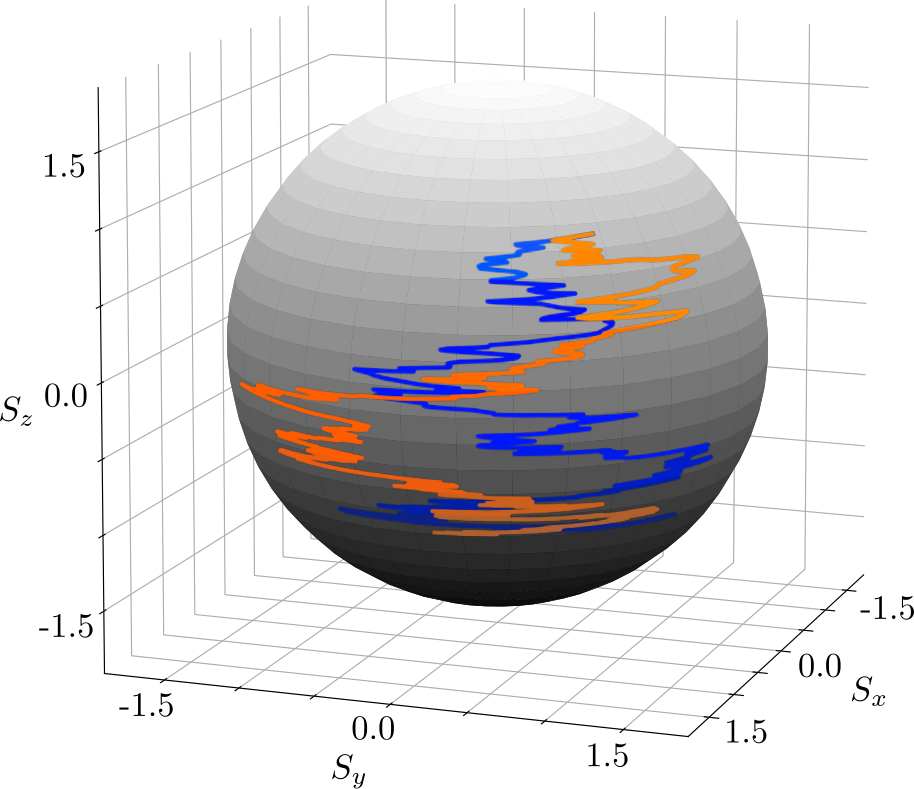
where $\theta_{m}(t),\phi_{m}(t)$ are the time-evolved trajectories and $M<\infty$ is the number of evolved trajectories and the overline denotes averaging over trajectories. As an example, in Fig. 1 we show two stochastic trajectories for the evaluation of the the dynamics of a single spin-$\frac{1}{2}$.

The above results for a single spin can be generalized to a system of $N>1$ spins by constructing the phase-space representation of the many-body density operator

where $\bm{\theta}=(\theta_{1},\ldots,\theta_{N})^{T}$, $\bm{\phi}=(\phi_{1},\ldots,\phi_{N})^{T}$ and $d\Omega_{n}=d\theta_{n}\sin\theta_{n}d\phi_{n}/2\pi$ pertains to the $n$th spin. A Pauli matrix $\hat{\sigma}_{n}^{\xi}$ ($\xi=x,y,z$) in the subspace of the $n$th spin acting on $\hat{A}(\bm{\theta},\bm{\phi})=\prod_{n}\hat{A}(\theta_{n},\phi_{n})$ generates the same operator-differential identities as in Eqs. (66). The FWF then becomes $\chi(\bm{\theta},\bm{\phi})=\left(\prod_{n=1}^{N}\frac{\sin\theta_{n}}{2\pi}\right)W(\bm{\theta},\bm{\phi})$.

Let us now consider interactions between the spins, e.g. of Ising type:

In analogy to the single spin approach, we derive equations for the time evolution of the phase-point operators first. The interactions then generate mixed-spin derivatives,

If only terms with derivatives in the same spin were present, the time evolution of an initially factorized operator $\hat{A}(t=0)=\prod_{n}\hat{A}_{n}(t=0)$ would preserve the factorization. But the terms with mixed-spin derivatives, such as the second and third term of Eq. (42) entangle the spins. Hence, in order to reproduce the DTWA, we have to discard all terms with mixed spin derivatives, $n\neq m$. We note that, in general, there is no a priori small parameter that justifies such a truncation and the validity of the truncation must be considered on a case-by-case basis. We will return to this issue in Sec. IV.5.

By repeating these steps for the von Neumann equation, we obtain a Fokker-Planck equation for the FWF $\chi({\bm{\theta}},{\bm{\phi}},t)$, resulting for the case of the Ising Hamiltonian in the set of ordinary differential equations for the spin angles

Transforming to Cartesian coordinates yields

which are precisely the mean-field EOMs for the Ising Hamiltonian in DTWA.

The coupling of spins to Markovian reservoirs can be straightforwardly included in our hybrid approach. Applying the mappings between the Hilbert space and phase space, Eq. (33), we have for the dephasing Lindbladian

Using a change of variables, we can transform the Fokker-Planck equation resulting from Eq. (45) to Cartesian coordinates, obtaining the set of SDEs

These equations reproduce Eqs. (13)-(15) of Ref. Huber et al. 2022 if we make the substitution $t\rightarrow 2t/\Gamma_{\phi}$.

In a similar way, we can derive the mappings for incoherent gains and losses,

Changing to Cartesian coordinates similarly reproduces the deterministic parts given by Eqs. (24) of Ref. Huber et al. 2022. One finds, however, that the diffusion matrix in Cartesian coordinates is not positive semidefinite and no corresponding SDE exists. In stark contrast to this, the parametrization with respect to $\theta,\phi$ does have a corresponding set of SDEs that can immediately be deduced from Eq. (47) as

Thus the hybrid discrete-continuous approach can incorporate incoherent processes which lead to classical noise terms in the EOMs.

We have seen in Sec. III that all pure spin states have a continuous SU(2) Wigner function $W(\theta,\phi)$ which is non-positive and thus cannot be sampled by Monte Carlo methods. This complicates explicit averaging over the initial Wigner distribution. This problem can be overcome by relating the continuous and discrete Wigner representations of spins using a gauge freedom Žunkovič 2015.

The SU(2) phase-point operators of Eq. (21) are orthogonal to all functions that only contain spherical harmonics $\text{Y}_{l,m}$ with $l\geq 2$,

which means that

The function $f$ can be chosen real by setting $C_{l,-m}=(-1)^{m}C_{l,m}$. Thus the representation of a spin state $\hat{\rho}$ in terms of a SU(2) Wigner function is not unique but has a gauge freedom

The initial discrete Wigner coefficients $W_{\bm{\alpha}0}$ are positive in many important cases. We now argue that the initial FWF $\chi_{0}(\theta,\phi)$ can be expressed in terms of $W_{\bm{\alpha}0}$ as

where the initial phase point operators $\hat{A}_{\bm{\alpha}}=\hat{A}(\theta_{\bm{\alpha}},\phi_{\bm{\alpha}})$ correspond to angles

Substituting this into Eq. (25a) reproduces the initial density operator. As an example, the spin down state is sampled from two points as

Next, it follows from the completeness relation of spherical harmonics,

that the difference between $\chi_{0}(\theta,\phi)$ of Eq. (52) and a directly evaluated FWF pertaining to the initial state contains only components of type $\sin(\theta)f(\theta,\phi)/2\pi$.

Using Eq. (52) and the fact that all eigenstates of the Pauli matrices have positive discrete Wigner coefficients $W_{\bm{\alpha}0}$, we can sample the initial phase space distribution from a discrete set of points. Using the discrete set of points decreases furthermore the statistical error when a finite number of samples is taken. Since all pure states (spin coherent states) are connected by unitary operations, we can generate positive discrete distributions for them as well. Finally, every mixed state can be represented as a mixture of pure states and therefore every single particle state is accessible by a classical Monte Carlo sampling.

The original formulation of the DTWA Schachenmayer et al. 2015 does not contain information on the range of validity of the interaction truncation. Instead, the quality of this approximation has only been characterized empirically, by comparing the predictions of the DTWA with exact (numerical) solutions for a given Hamiltonian. It was found in Ref. Schachenmayer et al. 2015 that the DTWA results reproduce the short time dynamics of macroscopic spin observables well if the interaction couples many spins in a similar way. We now provide an explanation for this empirical observation by deriving conditions under which the truncation approximation is justified.

Our aim is to show that the second and third derivatives in Eq. (42) generated by the two-body interactions of Eq. (41) can indeed be neglected in the case of macroscopic collective spin dynamics or for short interaction times. For simplicity, we assume the extreme limit of $J_{mn}=J$, i.e. consider all-to-all interactions. We then find that the FWF satisfies a PDE of the form

References

- Binder (2005) K. Binder, Monte-carlo methods, Mathematical tools for physicists , 249 (2005).
- Voter (2007) A. F. Voter, Radiation effects in solids, NATO Science Series (Springer, Berlin, 2007) , 1 (2007).
- Jin et al. (2016) J. Jin, A. Biella, O. Viyuela, L. Mazza, J. Keeling, R. Fazio, and D. Rossini, Cluster mean-field approach to the steady-state phase diagram of dissipative spin systems, Physical Review X 6, 031011 (2016).
- Weimer (2015) H. Weimer, Variational principle for steady states of dissipative quantum many-body systems, Physical review letters 114, 040402 (2015).
- Sieberer et al. (2016) L. M. Sieberer, M. Buchhold, and S. Diehl, Keldysh field theory for driven open quantum systems, Reports on Progress in Physics 79, 096001 (2016).
- Vidal (2004) G. Vidal, Efficient simulation of one-dimensional quantum many-body systems, Physical review letters 93, 040502 (2004).
- Verstraete et al. (2004) F. Verstraete, J. J. Garcia-Ripoll, and J. I. Cirac, Matrix product density operators: Simulation of finite-temperature and dissipative systems, Physical review letters 93, 207204 (2004).
- Cui et al. (2015) J. Cui, J. I. Cirac, and M. C. Bañuls, Variational matrix product operators for the steady state of dissipative quantum systems, Physical review letters 114, 220601 (2015).
- Wootters (1987) W. K. Wootters, A wigner-function formulation of finite-state quantum mechanics, Annals of Physics 176, 1 (1987).
- Schachenmayer et al. (2015) J. Schachenmayer, A. Pikovski, and A. M. Rey, Many-body quantum spin dynamics with monte carlo trajectories on a discrete phase space, Phys. Rev. X 5, 011022 (2015).
- Steel et al. (1998) M. J. Steel, M. K. Olsen, L. I. Plimak, P. D. Drummond, S. M. Tan, M. J. Collett, D. F. Walls, and R. Graham, Dynamical quantum noise in trapped bose-einstein condensates, Phys. Rev. A 58, 4824 (1998).
- Gardiner et al. (2004) C. Gardiner, P. Zoller, and P. Zoller, Quantum noise: a handbook of Markovian and non-Markovian quantum stochastic methods with applications to quantum optics (Springer Science & Business Media, 2004).
- Blakie et al. (2008) P. Blakie, A. Bradley, D. M.J., B. R.J., and G. C.W., Dynamics and statistical mechanics of ultra-cold bose gases using c-field techniques, Advances in Physics 57, 363 (2008).
- Polkovnikov (2010) A. Polkovnikov, Phase space representation of quantum dynamics, Ann. of Physics 325, 1790 (2010).
- Zhu et al. (2019) B. Zhu, A. M. Rey, and J. Schachenmayer, A generalized phase space approach for solving quantum spin dynamics, New Journal of Physics 21, 082001 (2019).
- Perlin et al. (2020) M. A. Perlin, C. Qu, and A. M. Rey, Spin squeezing with short-range spin-exchange interactions, Physical Review Letters 125, 223401 (2020).
- Czischek et al. (2018) S. Czischek, M. Gärttner, M. Oberthaler, M. Kastner, and T. Gasenzer, Quenches near criticality of the quantum ising chain—power and limitations of the discrete truncated wigner approximation, Quantum Science and Technology 4, 014006 (2018).
- Khasseh et al. (2020) R. Khasseh, A. Russomanno, M. Schmitt, M. Heyl, and R. Fazio, Discrete truncated wigner approach to dynamical phase transitions in ising models after a quantum quench, Physical Review B 102, 014303 (2020).
- Sundar et al. (2019) B. Sundar, K. C. Wang, and K. R. A. Hazzard, Analysis of continuous and discrete wigner approximations for spin dynamics, Phys. Rev. A 99, 043627 (2019).
- Kunimi et al. (2021) M. Kunimi, K. Nagao, S. Goto, and I. Danshita, Performance evaluation of the discrete truncated wigner approximation for quench dynamics of quantum spin systems with long-range interactions, Phys. Rev. Research 3, 013060 (2021).
- Polkovnikov (2003) A. Polkovnikov, Quantum corrections to the dynamics of interacting bosons: Beyond the truncated wigner approximation, Physical Review A 68, 053604 (2003).
- Huber et al. (2022) J. Huber, A. M. Rey, and P. Rabl, Realistic simulations of spin squeezing and cooperative coupling effects in large ensembles of interacting two-level systems, Phys. Rev. A 105, 013716 (2022).
- Huber et al. (2021) J. Huber, P. Kirton, and P. Rabl, Phase-space methods for simulating the dissipative many-body dynamics of collective spin systems, SciPost Physics 10, 045 (2021).
- Singh and Weimer (2022) V. P. Singh and H. Weimer, Driven-dissipative criticality within the discrete truncated wigner approximation, Phys. Rev. Lett. 128, 200602 (2022).
- Brif and Mann (1999) C. Brif and A. Mann, Phase-space formulation of quantum mechanics and quantum-state reconstruction for physical systems with lie-group symmetries, Phys. Rev. A 59, 971 (1999).
- Tilma et al. (2016) T. Tilma, M. J. Everitt, J. H. Samson, W. J. Munro, and K. Nemoto, Wigner functions for arbitrary quantum systems, Phys. Rev. Lett. 117, 180401 (2016).
- Saffman et al. (2010) M. Saffman, T. G. Walker, and K. Mølmer, Quantum information with rydberg atoms, Reviews of modern physics 82, 2313 (2010).
- Weimer et al. (2010) H. Weimer, M. Müller, I. Lesanovsky, P. Zoller, and H. P. Büchler, A rydberg quantum simulator, Nature Physics 6, 382 (2010).
- Wigner (1932) E. Wigner, On the quantum correction for thermodynamic equilibrium, Phys. Rev. 40, 749 (1932).
- Fano (1957) U. Fano, Description of states in quantum mechanics by density matrix and operator techniques, Rev. Mod. Phys. 29, 74 (1957).
- Hillery et al. (1984) M. Hillery, R.F.O’Connell, M. Scully, and E. Wigner, Distribution functions in physics: Fundamentals, Phys. Rep. 106, 121 (1984).
- Risken and Frank (1996) H. Risken and T. Frank, The Fokker-Planck Equation: Methods of Solution and Applications, Springer Series in Synergetics (Springer Berlin Heidelberg, 1996).
- Klimov and Chumakov (2009) A. B. Klimov and S. M. Chumakov, A group-theoretical approach to quantum optics: Models of atom-field interactions (John Wiley & Sons, 2009).
- Gardiner and Zoller (2010) C. Gardiner and P. Zoller, Quantum Noise: A Handbook of Markovian and Non-Markovian Quantum Stochastic Methods with Applications to Quantum Optics, Springer Series in Synergetics (Springer Berlin Heidelberg, 2010).
- Žunkovič (2015) B. Žunkovič, Continuous phase-space methods on discrete phase spaces, EPL (Europhysics Letters) 112, 10003 (2015).
- Browaeys and Lahaye (2020) A. Browaeys and T. Lahaye, Many-body physics with individually-controlled rydberg atoms, Nature Phys. 16, 132 (2020).
- Rackauckas and Nie (2017) C. Rackauckas and Q. Nie, Differentialequations.jl–a performant and feature-rich ecosystem for solving differential equations in julia, Journal of Open Research Software 5 (2017).
- Bezanson et al. (2017) J. Bezanson, A. Edelman, S. Karpinski, and V. B. Shah, Julia: A fresh approach to numerical computing, SIAM Review 59, 65 (2017).
- Pucci et al. (2016) L. Pucci, A. Roy, and M. Kastner, Simulation of quantum spin dynamics by phase space sampling of bogoliubov-born-green-kirkwood-yvon trajectories, Phys. Rev. B 93, 174302 (2016).
- Höning et al. (2013) M. Höning, D. Muth, D. Petrosyan, and M. Fleischhauer, Steady-state crystallization of rydberg excitations in an optically driven lattice gas, Phys. Rev. A 87, 023401 (2013).