english,Englishenglish,german,ngerman,french \DeclareSourcemap \maps[datatype=bibtex] \map \step[fieldset=addendum,null] \step[fieldset=eprintclass,null] \map \step[fieldsource=doi,final] \step[fieldset=url,null]
Real semi-stable degenerations, real-oriented blow-ups and straightening corners
Abstract
We study totally real semi-stable degenerations (and more generally, smooth semi-stable degenerations). Our goal is to describe the homeomorphism type of the real locus of the general fibre in terms of the special fibre. We give a general homeomorphism statement via the real-oriented blow-up of the family. Using this, we give more explicit descriptions of as a stratified space glued from (covers of) strata of the special fibre. We also give relative versions of the statements and consider the example of toric degenerations in order to link the technique to tropicalisation.
1 Introduction
Let be a complex semi-stable degeneration over the unit disc . Assume that is real, that is, is equipped with an anti-holomorphic involution compatible with complex conjugation on via . We say is totally real if locally each branch of the normal crossing divisor over is real, that is, fixed by the real structure. The detailed definitions can be found in the main text.
Theorem 1.1.
Let be a totally real semi-stable degeneration and let be the real-oriented blow-up of . We set and . Then there exists a homeomorphism
| (1) |
such that for all . In particular, the real positive special fibre is homeomorphic to the real locus of the generic real fibre , .
See [NO10, Theorem 5.1] and [Arg21, Proposition 6.4] for similar, more general, statements in the setting of log smooth maps and the Kato-Nakayama space (see below for more comments). We also prove the following relative version of this theorem.
Theorem 1.2.
Let be a totally real semi-stable degeneration and a transversal collection of real submanifolds. Then there exists a homeomorphism as in Theorem 1.1 such that
| (2) |
for all . In particular, the topological tuples and are homeomorphic for all .
In view of the above theorems, it is desirable to obtain concrete descriptions of the real positive special fibre . Note that in this text, strata of a stratification are always understood to be pairwise disjoint, locally closed subsets.
Theorem 1.3.
The real positive special fibre of a totally real semi-stable degeneration is a Whitney-stratified space whose strata are (the connected components of) topological covers of degree of each stratum of of codimension with respect to . In particular,
| (3) |
Here, is any refinement of the canonical normal crossing Whitney stratification on , but always denotes the codimension with respect to (see Section 7, page 7, for detailed definitions). In particular, if is a transversal collection of real divisors, we can choose to be the stratification induced by the normal crossing divisor .
A more explicit recipe for how the strata are glued together in can be found in Section 8 (especially for the case when all strata are simply connected).
Motivation and context
The idea of using simple (in this case, semi-stable) degenerations to study the generic fibre is of course very old and well-known. In particular, it is present from the very beginning in the topological study of real algebraic varieties. Axel Harnack’s and David Hilbert’s original “small perturbation” method [Har76, Hil91] is based on generic pencils of curves and hence semi-stable degenerations, see Section 5. A much more powerful incarnation of that idea was then introduced for hypersurfaces in toric varieties in the form of Oleg Viros’s patchworking method, see for example [Vir80, Vir06]. Again, semi-stable degenerations appeared at least implicitly in the proofs, e.g. [Vir06, Theorems 2.5.C and 2.5.D] and Section 9. We recommend [Vir] for a beautiful account of these ideas and their history. Other types of semi-stable deformations, in particular, deformations to the normal cone, see Section 5, are also commonly used in real algebraic geometry, often cleverly combined with Viro’s patchworking method, e.g. [Shu00, ST06, Bru+19]. Inspired by these results, in this paper we search for a “patchwork” description of the generic fibre for general semi-stable degenerations.
The connection to Viro’s patchworking will be made even more explicit in our upcoming joint work [RRS23] with Arthur Renaudineau and Kris Shaw. Based on our previous work [RRS22], we plan to apply the techniques of this paper to tropicalisations of families of real algebraic varieties . Inspired by the tropical description of Viro’s patchworking (cf. [Vir01, Mik04, IMS07]), the goal is to describe the homeomorphism type of the real locus of the generic fibre of in terms of its associated tropical variety equipped with a real phase structure , see [RRS22, Definition 2.2]. Under suitable smoothness assumptions, the situation can be reduced to semi-stable toric degenerations and hence to the statements in this paper, see Section 9. The idea to use the approach via real semi-stable degenerations was brought to our attention by Erwan Brugallé in his recent work [Bru22]. In this work, Brugallé uses the technique to prove that real algebraic varieties close to smooth tropical limits satisfy (the Euler characteristic of the real part is equal to the signature of the complex part), generalising previous works on patchworks in [Ite97, Ber10, BB07]. With Theorem 1.2 and Theorem 1.3 we provide the slightly refined ingredient for the argument on the Euler characteristic side.
Finally, one should mention that the techniques used here are in fact very similar to a significantly more general construction, studied in the language of logarithmic geometry, of the so-called Kato-Nakayama space or Betti realization associated to a log analytic space , see [KN99, (1.2)], also [NO10]. Indeed, if is the log space associated to a semi-stable degeneration, its Kato-Nakayama space coincides with the real-oriented blow-up, see [KN99, (1.2.3)]. The study of the real locus in presence of a real structure on is done in [Arg21]. In the overlap of the settings, Theorem 1.1 is a special incarnation of [NO10, Theorem 5.1] and [Arg21, Proposition 6.4].
Acknowledgement
My first thanks go to Arthur Renaudineau and Kris Shaw for the previous and ongoing collaborations which led me to this side project. Many joint conversations and discussions have inspired this text. Many thanks go to Erwan Brugallé for being the second source of inspiration, for many useful discussions on the subject, for corrections on earlier versions of the text and for sharing many ideas that entered here, in particular, Section 5 and Section 8. It is my special pleasure to thank Stefan Behrens for useful discussions and comments and for pointing me to the references and techniques that are crucial in the technical core of the paper in Section 4. I would also like to thank Lionel Lang for discussions on real-oriented blow-ups related to a different project, and Jean-Baptiste Campesato for mentioning to me early appearences of real-oriented blow-ups and his related works. Finally, I would like to thank Helge Ruddat and Hülya Argüz for pointing out to me the connections to logarithmic geometry and Kato-Nakayama spaces.
The author is supported by the FAPA project “Matroids in tropical geometry” from the Facultad de Ciencias, Universidad de los Andes, Colombia.
2 Smooth semi-stable degenerations
Our main statements are formulated in the context of complex semi-stable degenerations since the applications we have in mind are situated in this context. However, to a large extent our story takes places solely in the smooth manifolds of real points inside these degenerations. We hence start by setting up the corresponding framework of smooth semi-stable degenerations.
Let be a smooth manifold. A subset is called a normal crossing divisor if for any point there exists a chart centred in that identifies with for some . We refer to such a chart as normal crossing chart of type for at . Since any other chart at has the same type , we may also speak of the type of .
A smooth function is called a normal crossing function if for any point with there exists a chart centred in such that in local coordinates. Clearly, in such case is a normal crossing divisor. We refer to such a chart as normal crossing chart of type for at .
Definition 2.1.
A smooth semi-stable degeneration is a proper normal crossing function from a smooth manifold to the interval which is submersive over .
We denote the fibre over by . A generic fibre , , is a smooth submanifold of . The special fibre is a normal crossing divisor in . In fact, for most of what follows, it is sufficient to assume that is normal crossing but drop the condition that is normal crossing, see Section 7. Our goal is to understand the homeomorphism type of a generic fibre via data contained in the special fibre (and the degeneration, of course). A systematic way of doing so is using the language of real-oriented blow-ups.
Example 2.2.
We use the following simple example to illustrate the upcoming definitions and statements. For more interesting examples, we refer to later sections. We set and consider the map given by
Its two critical points are and . In the two-dimensional case, the existence of a chart at a critical point is clearly equivalent to the Hessian having negative determinant. Hence admits such a chart while does not. Since , it follows that the restriction to is a semi-stable degeneration, see Figure 1. Conversely, restriction of the shifted function does not yield a semi-stable degeneration.

3 Real-oriented blow-ups
We start by reviewing the notion of real-oriented blow-up along a normal crossing divisor. Our basic reference is [HPV00], early references are [ACa75, Per77].
Let be a smooth manifold and a normal crossing divisor. We denote by the real-oriented blow-up of along as defined in [HPV00, Definition 5.1, Proposition 5.2] (with the only difference that we are working in the smooth instead of real-analytic category here). For now, is a topological space (later, we will equip it with the structure of a manifold with corners) together with a blow-down map which is a homeomorphism over . It is unique up to canonical homeomorphism compatible with blow-down maps. In essence, is a space that behaves like minus a “tubular neighbourhood” of . Since the construction of the real-oriented blow-up is local, for our purposes it is enough to understand how it works on normal crossing charts. Note also that the following local description shows that is proper. We set and .
Lemma 3.1.
Set and for some . Then the real-oriented blow-up of along is given by
| (4) |
where the map on the first factors is given by the obvious map and on the last factors is identity.
Proof.
It will be convenient to label the orthants of in the following way: Given , we denote by the (closed) orthant in obtained as the closure of the set of points for which has sign for all . Clearly,
Whenever we want to explicitly specify the orthant that contains a point in , we write this point as a tuple , and .
The important fact for us is that real-oriented blow-ups are compatible with smooth semi-stable degenerations, that is, we can blow-up the map in the following sense.
Proposition 3.2.
Let be a smooth semi-stable degeneration. Let and denote the real-oriented blow-ups along the special fibre and along , respectively. Then there exists a unique continuous map such that the diagram
commutes. Moreover, is proper.
Proof.
It suffices to prove the statement on -normal crossing charts of type . Hence it is enough check the case , . By Section 3, the real-oriented blow-up is given by . Hence the only continuous map that agrees with on is given by
| (5) |
using the tuple notation from above. The properness follows easily from the fact that and are proper. �
Example 3.3.

Our main result in the framework of smooth semi-stable degenerations is the following theorem. We use the shorthand for the positive copy of zero in . The positive half-interval in is consequently denoted by for emphasis.
Theorem 3.4.
Let be a smooth semi-stable degeneration and let be the real-oriented blow-up of . We set and . Then there exists a homeomorphism
| (6) |
such that for all . In particular, and are homeomorphic for all .
4 Straightening corners
In order to prove Theorem 3.4, it is convenient to use the language of manifolds with corners and the well-known (though not well-documented) method of straightening corners.
The first systematic study of manifolds with corners appears in [Cer61, Dou61]. We will also use the references [Mel96, Joy12]. A (smooth) manifold with corners is a paracompact Hausdorff space covered by a maximal atlas of charts which are homeomorphisms between open sets in and open sets in containing . We call the type of the chart. The transition maps between charts are required to be smooth. Here, a smooth function on an open set is the restriction of a smooth function on an open set in containing . In particular, this guarantees that each point has a well-defined tangent space isomorphic to . For more details, we refer to [Mel96, Definition 1.6.1] and [Joy12, Section 2]. Note that [Mel96] calls the object of our definition t-manifolds and requires an additional global condition in his notion of manifold with corners.
A (strictly) inward-pointing vector field on a manifold with corners is a smooth vector field which, with respect to any chart of type , satisfies (or , respectively) for all (cf. [Mel96, Definition 1.13.10], [Joy12, Page 4]). By [Mel96, Corollary 1.13.1], an inward-pointing vector field can be integrated on compacts, that is, for any compact there exists and a smooth map
such that and .
A total boundary defining function on is a smooth function such that and for each point there exists a chart of type centred in such that in local coordinates (cf. [Mel96, Lemma 1.6.2], [Joy12, Definition 2.14]). Combining the flow of a strictly inward-pointing vector field with the level sets of a total boundary defining function, we obtain a way of smoothing the corners and turning into manifold with boundary. This construction can be found in various flavours and levels of details in the literature, for example, in [Wal16, Section 2.6, in particular 2.6.4] for (where additionally the uniqueness of the construction is discussed). For our purposes, the following statement is sufficient.
Theorem 4.1.
Let be a manifold with corners and let be a proper total boundary defining function. Then there exist and a (continuous) embedding
| (7) |
such that . In particular, and are homeomorphic for all .
Proof.
Since is proper, is compact. Fix a strictly inward-pointing vector field on . For existence, we can use to the existence of total boundary defining functions, see [Mel96, Lemma 1.6.2], whose gradients are strictly inward-pointing. More explicitly, we can argue as follows: First note that strictly inward-pointing vector fields exist locally in a chart. Moreover, sums and positive multiples of inward-pointing vector fields are inward-pointing. Hence using a partition of unity on (see [Mel96, Section 1.3 and Lemma 1.6.1]), we can construct an inward-pointing vector field on .
We denote by the integral flow associated to . Since is non-zero on , the image is a neighbourhood of . Since is proper, there exists such that is contained in this neighbourhood. Since is strictly inward-pointing and is a total boundary defining function, restricted to a flow line starting at is strictly increasing locally at . Hence, there exists such that restricted to a flow line is strictly increasing from value to value . We set and denote by the map which sends a point to the initial point of its flow line. We set . Clearly, is continuous. Moreover, it is bijective by our assumption that is strictly increasing on flow lines up to value . Since is compact and is Hausdorff, we conclude that is also continuous. Hence is the embedding required in the statement. �
Remark 4.2.
Let us comment on why we refer to the above embedding as “straightening corners”. Fix a smooth strictly increasing function such that and for . Using , we can construct a homeomorphism such that . Via we can equip with the structure of a manifold with boundary which coincides with the original structure away from the corner locus ().
We now explain how to apply straightening of corners to prove Theorem 3.4. A map between manifolds with corners is called smooth if pull-backs of smooth functions are smooth. This is the naive definition, see e.g. [Mel96, Equation (1.10.18)]. In the literature various refined notions exist, e.g. [Mel96, Section 1.12], [Joy12, Section 3]. Given a smooth map , we have induced differential maps for all defined as usual, and is called an immersion if is injective for all .
Lemma 4.3.
Let be a smooth manifold and a normal crossing divisor. Then the real-oriented blow-up carries a unique structure of manifold with corners such that is an immersion.
Proof.
Clearly, there exists a unique smooth structure on which satisfies the condition of the statement, namely the one induced from via . Moreover, the standard smooth structure on is the only one such that
is an immersion. By the description in Section 3 we can hence cover by open sets on which existence and uniqueness of such a structure holds. Finally, it is shown in [HPV00, Proposition 5.2] that the coordinate changes are smooth maps (between open sets in ). Hence the result follows. �
Lemma 4.4.
Let be a smooth semi-stable degeneration. Then the real-oriented blow-up is a smooth map between manifolds with corners. Moreover, the restriction
| (8) |
is a total boundary defining function for with boundary .
Proof.
Both statements are immediate consequences of the local description of given in Equation 5. �
Example 4.5.
Proof (Theorem 3.4).
By Section 4, carries the structure of a manifold with corners with boundary . By Section 4, is a proper total boundary defining function on . Let be an embedding as constructed in Theorem 4.1. Note that over , is proper and without critical values. Hence can be trivialised by Ehresmann’s theorem [Dun18, Theorem 8.5.10], that is, there exists a diffeomorphism such that and for all . Finally can be constructed using
| (9) |
�
5 Real semi-stable degenerations
We now return to the complex and real setting presented in the introduction. A notational warning: In this context, we will denote by the complex semi-stable degeneration. After adding a suitable real structure, the real sublocus forms a smooth semi-stable degeneration in the sense of the previous sections. So, the tuple from the previous sections will be replaced by now.
Definition 5.1.
A complex semi-stable degeneration is a proper holomorphic function from a complex manifold to the unit disc such that
- •
the map is regular at all ,
- •
the special fibre is a reduced normal crossing divisor.
The notions of normal crossing divisor/function as given in Section 2 admit obvious generalizations to the holomorphic setting. It is then clear that Section 5 and the holomorphic version of Section 2 agree: For any point , there exists an holomorphic chart centred in such that in local coordinates for some . We denote the tangent cone of at by . With respect to the chart from above, is just the union of the first hyperplanes.
Definition 5.2.
A real structure for is an orientation-reversing involution such that . The tuple is a real semi-stable degeneration. We say that is totally real if for any the differential fixes each hyperplane in the tangent cone .
Throughout the following, the letter indicates restriction to real points, that is, to the fixed points of a (given) real structure .
Lemma 5.3.
If is totally real, then the map is a smooth semi-stable degeneration.
Proof.
The definition implies that for any there exists a holomorphic normal crossing chart , for at such that corresponds to the standard (coordinate-wise) conjugation in . Clearly, the real locus of this chart , can be used as smooth normal crossing chart for . �
Example 5.4.
The smooth semi-stable degeneration from Section 2 is the real locus of the totally real semi-stable degeneration given by the same map allowing complex arguments and values (in ).
Example 5.5.
Section 2/Section 5 is a special case of the classical “small perturbation” method that was used in particular by Harnack and Hilbert to construct real projective curves with interesting topological properties, see [Har76, Hil91] and Figure 3. We refer to [Vir, Theorem 1.5.A] for more background. The construction can in fact be regarded as an example of semi-stable degenerations. The input for the small perturbation consists of two real projective curves and of degree such that
- •
the singularities of the real part are non-isolated nodes (that is, locally given by ),
- •
the real parts and intersect transversally (in particular, in non-singular points of and ).
We now consider the pencil of curves where and are homogeneous polynomials defining and , respectively. The method is then based on describing for small in terms of and certain combinatorial data (the pattern of signs of on ). Note that the conditions on the input data are essentially equivalent to the (smooth) semi-stability of the family
Moreover, in practice one can often assume that the conditions extend to complex points, that is, that additionally is nodal and and intersect transversally. In this case, the above degeneration is the real locus of the complex semi-stable degeneration
The requirement for the nodes of to be non-isolated is equivalent to the degeneration being totally real.

The present work can hence be regarded as an attempt to generalize the small perturbation method to arbitrary dimensions and the abstract setting. Note, however, that our methods would have to be modified in order to describe the topological pair (not just ). One approach would be to also degenerate and use the relative versions of our statements, c.f. Section 9.
Example 5.6.
A classical example of semi-stable degenerations are deformations to the normal cone [Ful98, Chapter 5]. Let by a compact complex manifold with real structure and a real submanifold. We denote by the (ordinary) blow-up of along . Then the canonical projection map is a totally real semi-stable degeneration. The generic fibre is , while the special fibre consists of and the projective completion of the normal bundle of in , that is, . These two components intersect in the exceptional divisor of and the section at infinity of which is the projective normal bundle . Note that if is a divisor, then and .
Given a normal crossing divisor in a complex manifold, we can apply the more general definition of real-oriented blow-up given in [HPV00] to regarded as real-analytic (sub-)varieties. However, the outcome has a simple description in terms of polar coordinates which allows us to avoid discussing the general definition. Again, it is sufficient to understand the local case. We denote by the unit circle in .
Lemma 5.7.
Set and for some . Then the real-oriented blow-up of along is given by
| (10) |
where the map on the first factors is given by
| (11) |
and on the last factors is identity.
Proof.
Again, the construction of real-oriented blow-ups can be applied to (suitable) families of complex varieties. This is discussed in detail in [ACG11, Chapter X, §9 and Chapter XV, §8] in the case of curves. More generally, given a complex semi-stable degeneration , we can construct the real-oriented blow-up which locally looks like
| (12) |
Proof (Theorem 1.1).
When is totally real, the blown-up family carries an induced real structure given, in local charts and coordinate-wise, by , . The relation to the blow-up of is the expected one: We have and . Hence, Theorem 1.1 is the consequence of applying Theorem 3.4 to the smooth semi-stable degeneration . �
6 The relative version
Given a smooth semi-stable degeneration , for any point with the tangent cone is a union of a finite number of hyperplanes . Note that if or if is a generic point of . A collection of closed submanifolds is called transversal if for each the collection of subspaces is transversal. That is, we require the codimension of
to be the sum of the codimensions of the individual spaces.
Theorem 6.1.
Let be a smooth semi-stable degeneration and a transversal collection of submanifolds.
- (a)
For any such that the intersection is non-empty, the restriction is a semi-stable degeneration.
- (b)
There exists a homeomorphism as in Theorem 3.4 such that for each we have
Proof.
Part (a): Assume that is non-empty. Since is closed in , the restriction is a proper map. Transversality of the ensures that is a submanifold. Transversality of and for ensures that is regular over . Finally, for , we can find numbers and a normal crossing chart for centred in such that in local coordinates
| (13) |
Here, it is understood that means that . Hence the restriction of this chart to corresponds to setting some coordinates , , to zero and hence provides a normal crossing chart for at .
Part (b): Using again the normal chart from Equation 13, we first observe that the real-oriented blow-up of is in fact equal to the total transform . It now suffices to choose the vector field that is used in the proof of Theorem 4.1 in a more specific manner. More precisely, we require for any with that is contained in . From Equation 13, it is clear that such a vector field exists locally. Since the required property is invariant under rescaling, we can use partition of unity to obtain a global vector field with the required property. We refer to [Mel96, Section 1.3] and [Cer61, Section 1.2.6] for a discussion of partitions of unity on manifolds with corners. Now, following the procedure in the proof of Theorem 4.1 we obtain flow lines for which is an invariant and hence the map satisfies for all . Combining this with the relative version of Ehresmann’s theorem, we can conclude as in the proof of Theorem 3.4. �
Let be a complex semi-stable degeneration. A collection of closed complex submanifolds is called transversal if it satisfies the same condition as in the smooth case, applied to the complex subspaces of . As in the proof of Part (a) of Theorem 6.1, we conclude that the restrictions are complex semi-stable degenerations. With these definitions, Theorem 1.2 is now a simple corollary of Theorem 6.1.
Proof (Theorem 1.2).
Given a point , we may use the complex version of the normal chart in Equation 13 (with the canonical real structure) to conclude that is totally real for all and that the collection is a transversal collection in the smooth sense. Hence the statement follows from Theorem 6.1. �
7 Stratifying the special fibre
Let be a smooth manifold and a normal crossing divisor. For a point , any normal crossing chart centred in is of the same type . We call the codimension of in . The codimension skeleton is the set of points of codimension at least . In particular and . The successive complements (the locus of points of codimension equal to ) are locally closed submanifolds of . A connected component is called a stratum of codimension of . Clearly is the disjoint union of all these strata. Moreover, the strata satisfy the Whitney condition, see [GM88, Part I, Section 1.2]. Indeed, since the condition is local, it suffices to check it for a normal crossing chart where it is obvious. Hence defines a Whitney stratification on in the sense of [GM88, Part I, Section 1.2]. We denote the set of strata by .
From now on, we denote by a Whitney stratification that refines . In our applications, the refinement will be equal to where is a normal crossing divisor containing . For any , we denote by the codimension of the unique stratum in that contains . In other words, is the number of sheets of that intersect in a point . Let be the real-oriented blow-up of along . We set for any and denote by the Euler characteristic with closed support.
Theorem 7.1.
The real-oriented blow-up of along a normal crossing divisor is a Whitney-stratified space via (the connected components of)
Moreover,
| (14) |
Proof.
Any manifold with corners, hence also , carries a canonical Whitney stratification (given again by codimension of points) denoted by . The map is a stratified map with respect to and , that is, the image of a stratum in is a stratum in and the restriction of to these strata is a submersion. In fact, in our situation such a restriction is also an immersion and hence a covering map. In particular, the (connected components) of the form a refinement of . Moreover, the restriction is a smooth covering map of degree with . All these statements can be checked immediately using the local description of in Equation 4. Hence
| and |
for with , which proves the theorem. �
Example 7.2.

In the case of a smooth semi-stable degeneration , we can restrict the previous discussion to the positive part. For any we set .
Corollary 7.3.
The positive special fibre of a smooth semi-stable degeneration is a Whitney-stratified space via (the connected components of)
Moreover,
| (15) |
Proof.
The statement follows from Theorem 7.1 plus the observation (see Equation 5) that for any , the subset of preimages such that consists of exactly half the points, that is, elements. �
Proof (Theorem 1.3).
Example 7.4.
Using the notation from Section 5, let us consider the semi-stable degeneration given by the deformation of to the normal cone of a line . In this case the special fibre consists of the two components and glued along . Hence the stratification of consists of the three strata , and . Clearly, we have and since . The map , however, is the connected degree covering map of (here ). Indeed, note that the normal bundles and are Möbius strips. The Euler characteristic computation in this case reads as
Remark 7.5.
At this point, it might be worthwhile to mention that most of what we did also works under the weaker assumption that is a weakly semi-stable. Here, a weakly semi-stable degeneration is a degeneration such that the total space is smooth, is regular away from , and is a normal crossing divisor, and is of finite order at (e.g. is real-analytic), but not necessarily normal crossing, that is, not necessarily reduced at . In other words, a weakly semi-stable degeneration has the local form
for some positive integers . Using these local charts, it is straightforward to check that all statements made until (including) Theorem 7.1 remain true without change. Section 7 can be adapted to weakly semi-stable degenerations as follows: The local form from above can be subdivided into three cases,
| (16) | ||||||
Given a stratum , the covering map is of degree , or , respectively, depending on the associated local form in the above order.
8 Gluing the special fibre
Let be a smooth manifold with normal crossing divisor . In applications, it is of interest to provide a more explicit description of how the various strata are glued together to form and , respectively. To do so, it is useful to introduce a few more definitions. Fix with . For any , the preimage can be canonically identified with the orthants near given by
| (17) |
Given a chart of type at , we get a canonical bijection between and which then yields a bijection to . In particular, . In the case of a smooth semi-stable degeneration , we can additionally define the subset of positive orthants given by
| (18) |
For , this subset can be canonically identified with and hence .
In general, in order to describe how the various strata are glued together, the monodromy of the covering maps has to be taken into account. For simplicity, we restrict our discussion here to the case of simply connected strata (or if we know for some other reason that the monodromy is trivial). A stratification is called simply connected if all its strata are simply connected. From now we assume that is simply connected. This implies, of course, that is a trivial covering map of whose sheets are labelled by . Moreover, in the semi-stable degeneration case, we have .
Given a stratum and a point , we define the ends of in by
| (19) |
Given another point in the same stratum as and a continuous path connecting the two, we get induced identifications of and as well as and . Since is simply connected, these identifications do no depend on the path. Hence we allow ourselves to write , and in the following. Note that corresponds to self-intersections of in , c.f. Figure 2 and Figure 5. We have a canonical orthant map
| (20) |
defined as follows: Consider a normal crossing chart of type centred at a point in . Via such a chart, corresponds to the orthants of . An end corresponds to a face of the subdivision of given by the coordinate hyperplanes. Finally, the orthants adjacent to can be canonically identified with . Then is the map corresponding to the inclusion.
The endpoint modification of is the map whose fibre over is . We can equip with a natural topology by requiring that is continuous and a sequence converges to if it converges to (in ) and, for each , the lie in the component of specified by , for large . We assume from now on that for some normal crossing divisor containing . In this case, using normal crossing charts we check easily that carries the structure of a manifold with corners that turns into a stratified smooth map with respect to . For more details, we refer to [HPV00, Page 235], [Joy12, Definition 2.6] and [Dou61, Section 6]. Note that is equivalent to for some which as mentioned above corresponds to self-intersections, see Figure 5 for an example.
Theorem 8.1.
The real-oriented blow-up of along a normal crossing divisor is the Whitney-stratified space obtained from gluing
via the maps
| (21) |
The positive special fibre of a smooth semi-stable degeneration is the Whitney-stratified space obtained from gluing
| (22) |
via the same maps restricted to positive orthants. In particular, in this case for all , .
Proof.
This is a consequence of the preceding discussion, except for possibly the last point: In the case of a semi-stable degeneration, given we may use a normal crossing chart for (of type ) to define . Then the positive orthants for both and are the orthants on which is positive. Hence respects positivity. �
Example 8.2.

Remark 8.3.
Let us make a few remarks.
- (a)
Of course, we could alternatively describe the gluing starting only with strata of maximal dimension. For example, is the space obtained from
via the following equivalence relation: Two points
are declared equivalent if , and .
- (b)
The situation is even simpler if we additionally assume that is strictly normal crossing, that is, all its irreducible components are smooth submanifolds of . Here, we use the adhoc definition of irreducible component as union of closures of maximal strata that are connected in codimension . In this case, for we have . Hence we have a canonical inclusion and . We then glue and along for sheets labelled by and if and only if .
- (c)
The orthant sets carry the structure of affine spaces with tangent space , where and is the set of hyperplanes in for a points . The maps are affine maps. The positive orthants form an affine hyperplane tangent to the hyperplane of points in whose coordinates sum up to zero.
- (d)
Again, Theorem 8.1 generalises to the case of weakly semi-stable degenerations from Section 7. The only change is that now, according to the three cases in Equation 16, we have , or , respectively. However, the orthant maps still respect positive orthants and the gluing can still be described as above.
Example 8.4.
Using the notation from Section 5, let us consider the semi-stable degeneration given by the deformation of to the normal cone of a conic . In this case the special fibre consists of the two components and (the fourth Hirzebruch surface) glued along . Note that is a topological -torus. Hence the stratification of consists of the strata , the two connected components of (a disc and a Möbius strip ) and (a cylinder). In contrast to Section 7, the normal bundles are (topologically) trivial and hence is the trivial (disconnected) covering map of degree . In particular, even though the stratification is not simply connected, there is no monodromy and we can directly apply Theorem 8.1. The stratified space is depicted in Figure 6.
We see that this deformation can potentially be used to “embed” real algebraic curves in (in particular, those which do not intersect ) inside . For example, in [Che02, Ore02] certain real algebraic curves in are used to construct new -curves of degree in . The transfer of these curves from to is achieved via the perturbation of the singularity of four maximally tangent conics which can also be interpreted/realized via the above deformation to the normal cone, c.f. [Shu00, Section 7] and [ST06, Chapter 3]. In the latter papers, deformations to the normal cone are used systematically to transfer a local deformation of singularities to a deformation of the whole curve. In [Bru+19, Proposition 4.7], the deformation to the normal cone of a cubic curve is used to construct a real algebraic curve of degree 12 such that consists of 45 isolated points. (Of course, in all these examples additional deformation-theoretic arguments are needed to prove that, in our notation, a given curve can be extended to a transversal in the sense of Theorem 1.2).
Interestingly, in contrast to Section 7, deformations to normal cones of curves of higher degree are not of Viro patchworking type, cf. Section 9. In particular, the embedding steps mentioned above cannot be directly achieved via patchworking (while patchworking is used for example in [Che02, Ore02] to construct the curves in to start with). My thanks go to Erwan Brugallé for sharing and explaining these ideas to me.
9 Toric degenerations
We now consider the particular case of toric degenerations (we use the term in the sense that is required to be a toric morphism). This example is not necessarily of interest by itself since it can be treated more directly, but it serves as an important ambient framework for applying our method in the context of tropicalisation as in [Bru22] and our upcoming joint work [RRS23]. We recall quickly the setup. More details can be found in [Smi96, Spe08].
Let be a finite complete polyhedral subdivision of . We denote by the fan in obtained by taking the cone over and completing it on level by the recession fan of . We call unimodular if is unimodular (in particular, is -rational in such case). We call strongly unimodular if the last coordinate of the primitive generator of any ray of is either or (in particular, is -rational in such case). This can be rephrased as follows: for every there exists and a part of a lattice basis such that
| (23) |
Note that for any unimodular there exists an integer such that is strongly unimodular.
We denote by and the complex and real toric varieties associated to . We denote by the canonical toric morphism corresponding to the projection to the last coordinate . Its generic fibre is equal to the , the toric variety associated to the recession fan. The special fibre is a union of torus orbits labelled by the cells and naturally identified with the group of semigroup homomorphisms
| with real locus |
The closure of such a complex or real torus orbit is denoted by and , respectively, and is equal to the complex or real toric variety associated to the star fan around denoted by . We denote by the tangent space of a rational polyhedron intersected with and set for any field
Note that .
If is unimodular, the variety is smooth, the map is regular away from and is a normal crossing divisor. In other words, in such case is weakly semi-stable.
Lemma 9.1.
If is strongly unimodular, is a totally real semi-stable degeneration.
Proof.
This seems to be well-known, we sketch the argument showing that is normal crossing. Given , let
denote the primitive generators of the rays of . Let linear forms on defined over such that and for all . These linear forms correspond to monomial functions in a neighbourhood of generating the ideals of the irreducible components of containing . In the same way, the projection corresponds to the function . But on , which proves that is normal crossing locally around . �
Remark 9.2.
If is unimodular, we can write
for positive integers which correspond to the integers mentioned in Section 7. Note that since is primitive, at least one of the is odd and hence all local forms are of the first type as listed in Equation 16. Hence the positive orthants behave as in the semi-stable case and the following discussion also applies to the weakly semi-stable case. In fact, the discussion in principle even applies to general subdivisions , but we do not need this here.
We assume from now on that is strongly unimodular. The toric boundary divisors of (that is, the rays of ) give rise to a transversal collection of smooth divisors . We denote by the stratification of associated to the normal crossing divisor
By construction, is a refinement of . We denote by the subset of strata contained in . These strata are exactly the connected components of the real torus orbits , hence they are (open) orthants. Moreover, these orthants are naturally labelled by the elements of . In summary, the strata in are labelled by tuples with and .
The semigroup homomorphisms of absolute value and logarithm induce maps and which we denote by the same symbols by abuse of notation. Note that here is the additive (semi-)group and hence is the group of ordinary linear homomorphisms For each stratum labelled by , this yields canonical homeomorphisms
Note that the normal crossing divisor is strictly normal crossing. In particular, the endpoint modification of a stratum is equal to the closure in , see Section 8. In fact, if is labelled by , it is sufficient to take the closure in , hence is a closed orthant of homeomorphic to the positive closed orthant. The latter can be described via the usual semigroup formalism for toric varieties, but using the (multiplicative) semigroup . This leads as naturally to tropical toric varieties which are defined using again the same formalism, but this time using the additive semigroup , see [Pay09, Section 3] and [MR19, Chapter 5]. Note that the extended logarithm map (setting ) is a semigroup isomorphism and a homeomorphism. It follows that the tropical variety associated to a fan is canonically homeomorphic to any closed orthant of the corresponding real toric variety. Applied to our situation, the statement is that is canonically homeomorphic to , the tropical toric variety associated to with open dense (tropical) torus .
Corollary 9.3.
The space is obtained from
| (24) |
via gluing generated by the following: Given pairs and , we identify with the copy contained in if
| and | under |
Proof.
The statement is the result of applying Theorem 8.1 to our particular case. In order to see this, it is enough to understand how the initial space from Equation 24 is identified with the initial space from Equation 22. To this end, let us give a more intrinsic description of the orthants of a stratum labelled by . It is useful to first study the set of orthants with respect to the divisor (instead of for ). In fact, note that the maximal strata of (equivalently, the orthants of ) are globally labelled by . Given , the tangent cone consists of hyperplanes which are naturally labelled by the rays of (the cone over ). The action on given by crossing a hyperplane (denoted by in Section 8) under this identifications corresponds to the additive action of the the subspace . Hence is an affine subspace in with tangent space . In fact, we can check easily that
where denotes the quotient map
Now, in order to pass from to , we just have to quotient by the subaction corresponding to the divisors among that contain . These correspond to the rays in , where denotes the recession cone of . In summary,
| with |
Finally, let us restrict to positive orthants. Clearly, the set of positive orthants in is the kernel of the map given by summing all coordinates. By projecting to the first coordinates, we can hence identify positive orthants with . With this last identification, we obtain
| with |
Summing over all strata labelled by a fixed of sedentarity , we obtain
This provides the identification between the two initial spaces in question. It is straightforward to check that the gluing described in Theorem 8.1 coincides with the gluing described here. �
Example 9.4.
The degeneration from Section 7 is in fact a toric degeneration induced by the subdivision depicted in Figure 7. Moreover, this subdivision is dual to a convex subdivision of a lattice polytope as used in Viro’s patchworking, cf. Section 9. Note that in contrast to the stratification discussed in Section 7, the stratification that takes into account the toric divisors is simply connected and the gluing procedure is described by Section 9.

As final ingredient of our discussion, we now add a real submanifold such that is a collection of transversal submanifolds. We call such a torically transversal. For any stratum labelled by (we do not change the stratification), we denote
Using the identifications from above, we consider these sets as subsets of and , respectively. We state for convenience the following summary which is just the combination of Theorem 1.2 and Section 9 applied to our case.
Corollary 9.5.
The topological pair is obtained via gluing as described in Section 9 from the topological pair
Here, denotes the projection to . Moreover, the topological pair is homeomorphic to for all and these homeomorphisms can be chosen such that they respect the intersections with the divisors .
Example 9.6.
Viro’s patchworking method [Vir80, Vir06] takes as input a Laurent polynomial in variables and a convex subdivision of the Newton polytope of (induced by a piecewise linear convex function ; we may assume that takes integer values on integer points). The associated Viro polynomial is
For , we denote by the closure of in , the toric variety associated to .
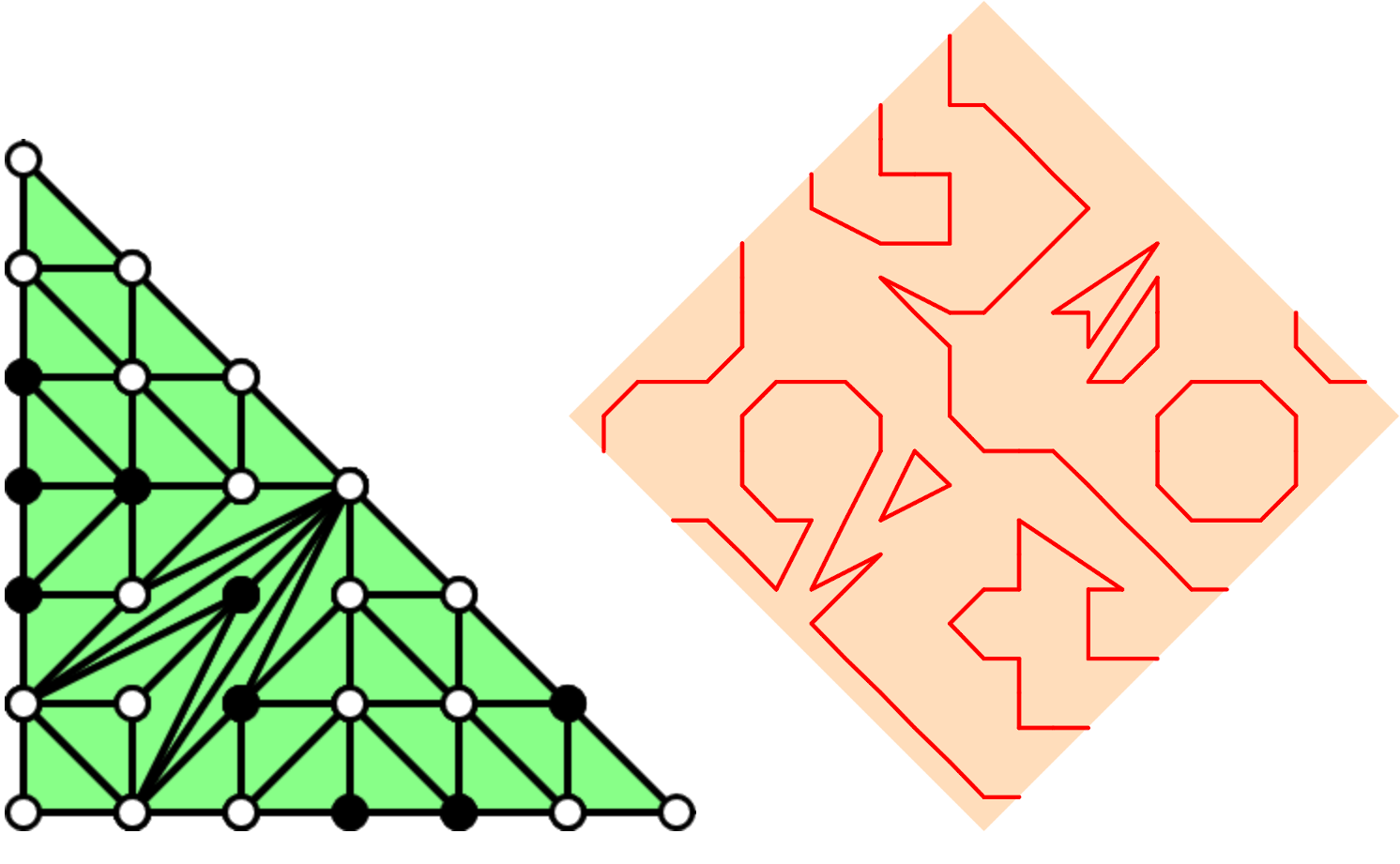
Let us furthermore assume that is non-degenerate, that is, for any the truncation defines a non-singular hypersurface in . Under this assumption, Viro’s patchworking theorem [Vir06, Theorem 1.7.A] provides a description of for small values of in terms of gluing patches given by the truncations , . An example of the particular case of combinatorial unimodular patchworking (that is, is a unimodular triangulation of ) is depicted in Figure 8. The connection to our setup is as follows: Let the upper graph of the convex function associated to . Let be a desingularisation of , that is, the normal fan of is unimodular and refines the normal fan of . Then the projection to induces a map which is a toric totally real weakly semi-stable degeneration with generic fibre as explained above. Moreover the closure of in is a real submanifold which is torically transversal. This is essentially the statement of [Vir06, Theorem 2.5.C], even though the terminology of semi-stable (and toric) degenerations is not used explicitly there. Hence our methods recover/reformulate parts of Viro’s patchworking method (see [Vir06, Theorem 3.3.A] for connecting the gluing from Section 9 with respect to the desingularisation to the patchwork described in [Vir06, Section 1.5]). We hope to generalise this to tropicalisations of arbitrary codimension in our upcoming joint work [RRS23] with Arthur Renaudineau and Kris Shaw.
References
- [ACa75] Norbert A’Campo “La fonction zeta d’une monodromie” In Comment. Math. Helv. 50.1, 1975, pp. 233–248 DOI: 10.1007/BF02565748
- [ACG11] Enrico Arbarello, Maurizio Cornalba and Phillip. Griffiths “Geometry of algebraic curves. Volume II” 268, Grundlehren Math. Wiss. Springer Berlin Heidelberg, 2011, pp. 928 DOI: 10.1007/978-3-540-69392-5
- [Arg21] Hülya Argüz “Real loci in (log) Calabi-Yau manifolds via Kato-Nakayama spaces of toric degenerations” In Eur. J. Math. 7.3, 2021, pp. 869–930 DOI: 10.1007/s40879-021-00454-z
- [Ber10] Benoit Bertrand “Euler characteristic of primitive -hypersurfaces and maximal surfaces” In J. Inst. Math. Jussieu 9.1, 2010, pp. 1–27 DOI: 10.1017/S1474748009000152
- [BB07] Benoit Bertrand and Frederic Bihan “Euler Characteristic of real nondegenerate tropical complete intersections” In ArXiv e-prints, 2007 arXiv:0710.1222
- [Bru22] Erwan Brugallé “Euler characteristic and signature of real semi-stable degenerations” In J. Inst. Math. Jussieu Cambridge University Press (CUP), 2022, pp. 1–8 DOI: 10.1017/s1474748022000056
- [Bru+19] Erwan Brugallé, Alex Degtyarev, Ilia Itenberg and Frédéric Mangolte “Real algebraic curves with large finite number of real points” In Eur. J. Math. 5.3 Springer, New York, NY, 2019, pp. 686–711 DOI: 10.1007/s40879-019-00324-9
- [Cer61] Jean Cerf “Topologie de certains espaces de plongements” In Bull. Soc. Math. France 89 Société Mathématique de France (SMF), Paris, 1961, pp. 227–380 DOI: 10.24033/bsmf.1567
- [Che02] Benoit Chevallier “Four -curves of degree 8” In Funct. Anal. Appl. 36.1 Springer US, New York, NY, 2002, pp. 76–78 DOI: 10.1023/A:1014442620363
- [Dou61] Adrien Douady “Variétés à bord anguleux et voisinages tubulaires” In Semin. H. Cartan 14.1, 1961, pp. 1–11 URL: http://eudml.org/doc/112429
- [Dun18] Bjørn Dundas “A short course in differential topology”, Camb. Math. Textb. Cambridge: Cambridge University Press, 2018 DOI: 10.1017/9781108349130
- [Ful98] William Fulton “Intersection theory” Berlin: Springer, 1998, pp. 470 DOI: 10.1007/978-1-4612-1700-8
- [GM88] Mark Goresky and Robert MacPherson “Stratified Morse theory” 14, Ergebnisse der Mathematik und ihrer Grenzgebiete. 3. Folge Springer Berlin Heidelberg, 1988, pp. 272 DOI: 10.1007/978-3-642-71714-7_1
- [Har76] Axel Harnack “Ueber die Vieltheiligkeit der ebenen algebraischen Curven” In Math. Ann. 10 Springer, Berlin/Heidelberg, 1876, pp. 189–199 DOI: 10.1007/BF01442458
- [HRR17] Boulos Hilany, Johannes Rau and Arthur Renaudineau “Combinatorial patchworking tool”, 2017 URL: https://math.uniandes.edu.co/˜j.rau/patchworking/patchworking.html
- [Hil91] David Hilbert “Ueber die reellen Züge algebraischer Curven” In Math. Ann. 38 Springer, Berlin/Heidelberg, 1891, pp. 115–138 DOI: 10.1007/BF01212696
- [HPV00] John Hubbard, Peter Papadopol and Vladimir Veselov “A compactification of Hénon mappings in as dynamical systems” In Acta Math. 184.2 International Press of Boston, Somerville, MA; Institut Mittag-Leffler, Stockholm, 2000, pp. 203–270 DOI: 10.1007/BF02392629
- [Ite97] Ilia Itenberg “Topology of real algebraic -surfaces” In Revista Matemática de la Universidad Complutense de Madrid 10, 1997, pp. 131–152 URL: http://eudml.org/doc/44256
- [IMS07] Ilia Itenberg, Grigory Mikhalkin and Eugenii Shustin “Tropical algebraic geometry” 35, Oberwolfach Semin. Birkhäuser Basel, 2007, pp. 103 DOI: 10.1007/978-3-0346-0048-4
- [Joy12] Dominic Joyce “On manifolds with corners” In Advances in geometric analysis. Collected papers of the workshop on geometry in honour of Shing-Tung Yau’s 60th birthday, Warsaw, Poland, April 6–8, 2009 Somerville, MA: International Press; Beijing: Higher Education Press, 2012, pp. 225–258 arXiv:0910.3518
- [KN99] Kazuya Kato and Chikara Nakayama “Log Betti cohomology, log étale cohomology, and log de Rham cohomology of log schemes over ” In Kodai Math. J. 22.2, 1999, pp. 161–186 DOI: 10.2996/kmj/1138044041
- [Mel96] Richard Melrose “Differential analysis on manifolds with corners” Unfinished, 1996 URL: https://klein.mit.edu/˜rbm/book.html
- [Mik04] Grigory Mikhalkin “Amoebas of algebraic varieties and tropical geometry” In Different faces of geometry New York, NY: Kluwer Academic/Plenum Publishers, 2004, pp. 257–300 DOI: 10.1007/0-306-48658-X_6
- [MR19] Grigory Mikhalkin and Johannes Rau “Tropical Geometry”, textbook in preparation, 2019 URL: https://math.uniandes.edu.co/˜j.rau/downloads/main.pdf
- [NO10] Chikara Nakayama and Arthur Ogus “Relative rounding in toric and logarithmic geometry” In Geom. Topol. 14.4, 2010, pp. 2189–2241 DOI: 10.2140/gt.2010.14.2189
- [Ore02] Stepan. Orevkov “New -curve of degree 8” In Funct. Anal. Appl. 36.3 Springer US, New York, NY, 2002, pp. 247–249 DOI: 10.1023/A:1020118609560
- [Pay09] Sam Payne “Analytification is the limit of all tropicalizations” In Math. Res. Lett. 16.2-3 International Press of Boston, Somerville, MA, 2009, pp. 543–556 DOI: 10.4310/MRL.2009.v16.n3.a13
- [Per77] Ulf Persson “On degenerations of algebraic surfaces” 189, Mem. Am. Math. Soc. Providence, RI: American Mathematical Society (AMS), 1977 DOI: 10.1090/memo/0189
- [RRS22] Johannes Rau, Arthur Renaudineau and Kris Shaw “Real phase structures on matroid fans and matroid orientations” In J. Lond. Math. Soc. 106.4 Wiley, 2022, pp. 3687–3710 DOI: https://doi.org/10.1112/jlms.12671
- [RRS23] Johannes Rau, Arthur Renaudineau and Kris Shaw “Real phase structures and patchworking of tropical manifolds” In in preparation, 2023
- [Shu00] Eugenii Shustin “Lower deformations of isolated hypersurface singularities” In St. Petersburg Math. J. 11.5 American Mathematical Society (AMS), Providence, RI, 2000, pp. 883–908 (2000)and alebra anal. 11no. 5221–249
- [ST06] Eugenii Shustin and Ilya Tyomkin “Patchworking singular algebraic curves II” In Israel J. Math. 151 Springer, Berlin/Heidelberg; Hebrew University Magnes Press, Jerusalem, 2006, pp. 145–166 DOI: 10.1007/BF02777359
- [Smi96] A.. Smirnov “Torus schemes over a discrete valuation ring” In St. Petersburg Math. J. 8.4 American Mathematical Society (AMS), Providence, RI, 1996, pp. 161–172
- [Spe08] David. Speyer “Tropical linear spaces” In SIAM J. Discrete Math. 22.4 Society for IndustrialApplied Mathematics (SIAM), Philadelphia, PA, 2008, pp. 1527–1558 DOI: 10.1137/080716219
- [Vir80] Oleg Viro “Curves of degree 7, curves of degree 8, and the Ragsdale conjecture” In Soviet Mathematics. Doklady 22 American Mathematical Society (AMS), Providence, RI, 1980, pp. 566–570
- [Vir01] Oleg Viro “Dequantization of real algebraic geometry on logarithmic paper” In 3rd European congress of mathematics (ECM), Barcelona, Spain, July 10–14, 2000 1 Basel: Birkhäuser, 2001, pp. 135–146 DOI: 10.1007/978-3-0348-8268-2_8
- [Vir06] Oleg Viro “Patchworking real algebraic varieties” In ArXiv e-prints, 2006 arXiv:math/0611382
- [Vir] Oleg Viro “Introduction to Topology of Real Algebraic Varieties”, Unfinished URL: http://www.math.stonybrook.edu/˜oleg/easymath/es/es.html
- [Wal16] C.. Wall “Differential topology” 156, Cambridge Stud. Adv. Math. Cambridge: Cambridge University Press, 2016, pp. 346 DOI: 10.1017/CBO9781316597835
Contact
Johannes Rau
Departamento de Matemáticas
Universidad de los Andes
KR 1 No 18 A-10, BL H
Bogotá, Colombia
j.rau AT uniandes.edu.co