跳到论文正文
W Papers独立论文阅读器 arXiv:2203.16877 论文正文 计算阅读时间 · 0%
引用这篇论文根据当前论文元数据生成,正式投稿前建议核对。


License: CC Zero
arXiv:2203.16877v1 [math.AP] 31 Mar 2022

Asymptotic behavior of the Dirichlet energy
on Poisson point cloudsThanks: Preprint SISSA 06/2022/MATE

Andrea Braides Address: SISSA, via Bonomea 265, Trieste Email address: braides@mat.uniroma2.it and Marco Caroccia Address: Politecnico di Milano, Piazza Leonardo da Vinci, 32, 20133 Milano (MI) Email address: marco.caroccia@polimi.it
Abstract.

We prove that quadratic pair interactions for functions defined on planar Poisson clouds and taking into account pairs of sites of distance up to a certain (large-enough) threshold can be almost surely approximated by the multiple of the Dirichlet energy by a deterministic constant. This is achieved by scaling the Poisson cloud and the corresponding energies and computing a compact discrete-to-continuum limit. In order to avoid the effect of exceptional regions of the Poisson cloud, with an accumulation of sites or with ‘disconnected’ sites, a suitable ‘coarse-grained’ notion of convergence of functions defined on scaled Poisson clouds must be given.

Key words and phrases:
Poisson random sets, homogenization, discrete-to-continuum, Bernoulli percolation

1. Introduction

The object of this paper is an analysis of the asymptotic behaviour of quadratic energies on Poisson random sets. Loosely speaking such sets are characterized by the property that the number of their points contained in a given set has a Poisson probability distribution, and that the random variables related to disjoint sets are independent. Even more loosely, in average the number of points contained in a set is proportional to the Lebesgue measure of the set. We denote by η\eta such a random set.

In order to define some almost-sure properties of η\eta we use a discrete-to-continuum approach that has been fruitfully used to derive continuum theories from microscopic interactions (see [2]). A simple interpretation of this method is as a finite-difference approximation. If η\eta is a deterministic periodic locally finite discrete set in ℝd\mathbb{R}^{d}, then we can consider real-valued functions u:η→ℝu:\eta\to\mathbb{R} and quadratic interaction potentials between points on η\eta. The corresponding Dirichlet-type energy is

(1.1) ∑⟨x,y⟩(u⁡(x)−u⁡(y))2,\sum_{\langle x,y\rangle}(u(x)-u(y))^{2},

where ⟨x,y⟩\langle x,y\rangle indicates summation over nearest-neighbouring pairs (x,y)(x,y) in η\eta. We can then introduce a small parameter ε\varepsilon and scale both the environment and the energies accordingly; namely, considering u:ε​η→ℝu:\varepsilon\,\eta\to\mathbb{R} and

(1.2) ∑⟨x,y⟩εd−2​(u⁡(x)−u⁡(y))2,\sum_{\langle x,y\rangle}\varepsilon^{d-2}(u(x)-u(y))^{2},

now summing over nearest-neighbouring pairs (x,y)(x,y) in ε​η\varepsilon\,\eta. By letting ε→0\varepsilon\to 0 we obtain a limit continuum energy, of the form

(1.3) ∫ℝd𝐀∇u⋅∇udx,\int_{\mathbb{R}^{d}}{\bf A}\nabla u\cdot\nabla u\,{\rm d}x,

where the matrix 𝐀\bf A carries information about the microstructure of the original set η\eta. Note that in order to perform this passage to the limit we have to embed our energies in a common environment identifying functions on η\eta with suitable interpolations. The limit is meant in the sense of Γ\Gamma-convergence, which implies that minimum problems for the limiting energies are approximations of the discrete ones, and can also be performed ‘locally’, by considering interactions only for x∈ε​η∩Ux\in\varepsilon\eta\cap U for a fixed open set UU.

In order to define analogs of (1.1) and (1.2) for the realization of a Poisson cloud η\eta we face a choice regarding what to consider as ‘interacting sites’, whether nearest neighbours in the sense of Voronoi cells or points ‘close’ in the sense of the ambient space. For the random set η\eta these two choices are not equivalent since nearest-neighbouring points on η\eta may be indeed arbitrarily distant in the ambient space, and conversely a very small distance between points of η\eta does not ensure that they are nearest neighbours in η\eta. We choose the second option, which also seems closer to applications; namely, we introduce an interaction radius λ>0\lambda>0 and consider the energies

(1.4) ℱε​(u)=∑x,y∈Q∩ε​η,|x−y|<ε​λεd−2​(u⁡(x)−u⁡(y))2,\mathcal{F}_{\varepsilon}(u)=\sum_{\begin{subarray}{c}x,y\in Q\cap\varepsilon\eta,\\ |x-y|<\varepsilon\lambda\end{subarray}}\varepsilon^{d-2}(u(x)-u(y))^{2},

defined for u:ε​η∩Q→ℝu:\varepsilon\,\eta\cap Q\to\mathbb{R}, where QQ is the unit coordinate cube centered in 00 (for ease of notation we treat only this case, which anyhow, up to scaling and localization, implies the result for any bounded Lipschitz open set in ℝd\mathbb{R}^{d}). Note that, if a Γ\Gamma-limit of such energies does exist then, thanks to the invariance properties by rotations of η\eta, it must be a multiple of the Dirichlet integral (i.e., 𝐀\bf A in (1.3) is equal to a multiple of the identity matrix), which we expect to be almost surely deterministic.

Refer to caption
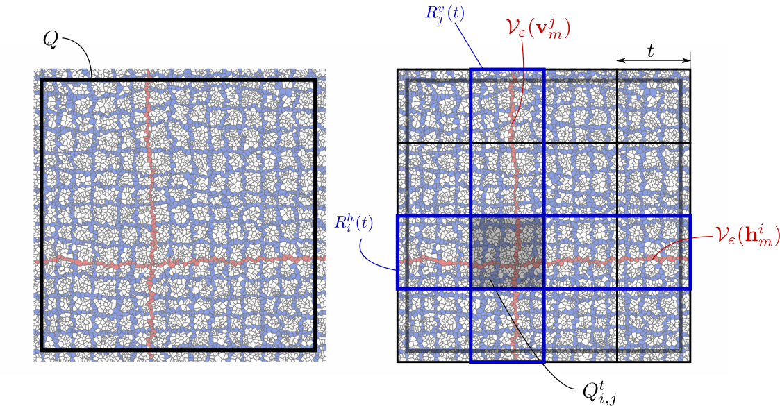
Figure 1.1. A representation of a regular grid in QQ with two ‘paths’ highlighted.

The main issue in proving the convergence of ℱε\mathcal{F}_{\varepsilon} consists in providing a suitable notion of convergence for discrete functions uεu_{\varepsilon} to a continuum parameter uu, for which a compactness theorem can be proved under an assumption of boundedness of the energies. While for periodic η\eta we can use piecewise-constant interpolations on Voronoi cells (or, equivalently, piecewise-affine interpolations on the related Delaunay triangulation), for a Poisson point process we cannot control the behaviour of such interpolation due to the presence of arbitrarily large and arbitrarily small Voronoi cells. Nevertheless, we can prove that the union of ‘regular’ Voronoi cells with suitably controlled dimensions form an infinite connected set in which we find ‘paths’ of cells such that also cells at distance λ\lambda are regular. This is done by exploiting a Bernoulli site-percolation argument. In the planar case d=2d=2 the complement of this set of Voronoi is composed of isolated sets with controlled dimensions, so that the ambient space can be thought of as a “perforated domain”, in which we do not have a control of the discrete functions only in isolated ‘holes’ of controlled size. This allows to define a suitable convergence by choosing a subset GεG_{\varepsilon} of ε​η\varepsilon\eta composed of paths mentioned above whose union 𝒱ε​(Gε)\mathcal{V}_{\varepsilon}(G_{\varepsilon}) has the geometry of a square grid (see Fig. 1.1) We thus use these grids to define a suitable convergence notion: given a sequence of function uε:ε​η→ℝu_{\varepsilon}:\varepsilon\,\eta\rightarrow\mathbb{R} we say that uu is the L2L^{2}-limit of uεu_{\varepsilon} if

(1.5) ∫𝒱ε​(Gε)|u^ε−u|2​𝑑x→0;\int_{\mathcal{V}_{\varepsilon}(G_{\varepsilon})}|\hat{u}_{\varepsilon}-u|^{2}\,\mathrm{d}x\rightarrow 0;

namely, if the L2L^{2}-distance between the piecewise-constant extensions u^ε\hat{u}_{\varepsilon} of uεu_{\varepsilon} and uu, restricted to the Voronoi cells of the grid GεG_{\varepsilon} vanishes as ε→0\varepsilon\rightarrow 0. Regular grids allow also to give a meaningful notion of boundary-value problems; in particular we can consider affine boundary condition as in the cell problems

(1.6) m(ξ;TQ):=inf{∑x∈η∩(T​Q)∑y∈η∩Bλ​(x)|v(x)−v(y)|2|v:η→ℝv⁡(x)=ξ⋅xfor all x∈η such thatdist⁡(x,∂(T​Q))≤2​λ}.\mathrm{m}(\xi;TQ):=\inf\left\{\sum_{x\in\eta\cap(TQ)}\sum_{y\in\eta\cap B_{\lambda}(x)}|v(x)-v(y)|^{2}\ \left|\begin{array}[]{c}v:\eta\rightarrow\mathbb{R}\\ \ v(x)=\xi\cdot x\ \ \text{\rm for all $x\in\eta$ such that}\\ \mathrm{dist}(x,\partial(TQ))\leq 2\lambda\end{array}\right.\right\}.

Using subadditive ergodic theorems we then can prove that, if ξ≠0\xi\neq 0, the constant Ξ\Xi given by

Ξ:=limT→+∞m⁡(ξ,T​Q)T2​|ξ|2\Xi:=\lim_{T\rightarrow+\infty}\frac{\mathrm{m}(\xi;TQ)}{T^{2}|\xi|^{2}}

exists and is deterministic. Moreover, by the invariance properties of η\eta it does not depend on ξ\xi. This allows to state and prove the main result of the paper, which is the almost sure Γ\Gamma-convergence in the planar case d=2d=2 of functionals (1.4) to

(1.7) ℱ⁡(u)=Ξ​∫Q|∇u|2​𝑑x\mathcal{F}(u)=\Xi\int_{Q}|\nabla u|^{2}{\rm d}x

with respect to the convergence in (1.5). Note that more in general we may consider energies of the form

(1.8) ℱεa​(u)=∑x,y∈Q∩ε​ηεd−2​a​(x−yε)​(u⁡(x)−u⁡(y))2,\mathcal{F}_{\varepsilon}^{a}(u)=\sum_{x,y\in Q\cap\varepsilon\eta}\varepsilon^{d-2}a\Bigl({x-y\over\varepsilon}\Bigr)(u(x)-u(y))^{2},

with aa positive and with compact support, recovering the case in (1.4) as a special case when a⁡(ξ)a(\xi) is the characteristic function of the ball centered in 00 and radius λ\lambda. If aa is radially symmetric the same limit result holds with obvious modifications in the statements.

The convergence theorem can be compared with various results in the literature. Our result is inspired by the recent paper [7], where perimeter energies on Poisson random sets are considered. In that context a simpler compactness result can be obtained with respect to the convergence is measure of sets, by using a covering lemma that ensures that the energy cannot concentrate on non-regular Voronoi cells. In the present context, this would correspond to an extension theorem for Sobolev functions from regular sets, which seems hard to obtain due to the random geometry of clusters of non-regular Voronoi cells. Furthermore, we can compare our approach to that in [4, 3], where a notion of stochastic lattice η\eta is given for which energies of the form (1.8) can be considered. Differently from Poisson random sets, stochastic lattices are more regular, in that all Voronoi cells have controlled dimension and hence are regular in the terminology above, a condition that seems a considerable restriction in terms of applications. The regularity of the lattice implies that functionals ℱεa\mathcal{F}_{\varepsilon}^{a} are coercive with respect to the L2L^{2} convergence of piecewise-constant interpolations on Voronoi cells. Conversely, in general the limits of functionals ℱεa\mathcal{F}_{\varepsilon}^{a}, which exist under ergodicity and stationarity assumptions, are not isotropic even if aa is radially symmetric, except for specially constructed examples [16]. More general random distributions of sites have been considered within problems in Machine Learning by D. Slepcev et al. [9, 12, 18] (see also the references therein). In their approach the convergence is given in terms of suitable interpolations of discrete functions using Optimal-Transport techniques. The presence of non-regular Voronoi cells is mitigated by considering kernels aεa^{\varepsilon} with increasing support as ε→0\varepsilon\to 0, which also allow to obtain isotropy in the limit (see also [8] for variational limits using a coarse-graining approach). Energies (1.8) have a continuum approximation in terms of a convolution double integral, for which random homogenization has been considered in [6] (see also [1]). We note that the existence of regular paths can be proved in any dimension d≥2d\geq 2, but if d>2d>2 the geometry of regular grids can be thought as a set of “fibers” rather than a perforated domain. We believe that the same asymptotic result holds but with an even more complex argument. Finally, we mention, following a remark by D. Slepcev in a private communication, that our results may also have practical implications for the study of the graph Laplacian. Namely, one can show that if one drops all of the eigenmodes of the graph Laplacian on a low degree random geometric graph where the eigenvector has large L∞L^{\infty} norm (in other words concentrates at few nodes) one still recovers the continuum spectrum.

We briefly outline the plan of the paper. In Section 2 we introduce the necessary definitions and notation for Poisson point clouds. This allows to give a definition of Dirichlet energy on a Poisson cloud η\eta and to prove some asymptotic properties as the Poisson set is scaled by a small parameter η\eta and correspondingly the energies ℱε\mathcal{F}_{\varepsilon} as in (1.4). We introduce the notation for Voronoi cells and define grids of paths of regular cells 𝒢ε,t{\mathcal{G}}_{\varepsilon,t} depending on an additional parameter t>0t>0. This allows to define the convergence of piecewise-constant functions uεu_{\varepsilon} on Voronoi cells to a continuum function uu as the successive convergence of averages of uεu_{\varepsilon} computed on 𝒢ε,t{\mathcal{G}}_{\varepsilon,t} at the “mesoscopic scale” tt to piecewise-constant functions utu^{t} defined on a square grid and then of such utu^{t} to a limit uu as t→+∞t\to+\infty (Definition 2.7). This is proved to be equivalent to the L2L^{2} convergence on grids as in (1.5), and actually independent of the choice of the family of grids. In Section 3 we state the main results of the paper. Theorem 3.1 states the pre-compactness the sense of the convergence above of sequences with equi-bounded Dirichlet energy; Theorem 3.3 is an almost-sure homogenization result characterizing the Γ\Gamma-limit of Dirichlet energies as a deterministic quantity as in (1.7). Section 4 is devoted to the proof of the Compactness Theorem, based on the geometric properties of the grids that allow the use of Poincaré inequalities. In Section 5 we prove the Homogenization Theorem. The lower bound is obtained by using the Fonseca and Müller blow-up method, which is possible thanks to the use of cut-off functions that are locally constant close to non-regular Voronoi cells. The construction of recovery sequences is also made possible thanks to these ‘regular’ cut-off functions. Finally Section 6 (the Appendix) contains the proof of the existence of regular grids.

2. Notation and preliminaries

In this section we introduce the main ingredients required to perform our analysis. For the sake of simplicity, and since our analysis will take place in this context, we always consider the ambient space dimension to be two-dimensional, even though some of the definitions and results can be extended to general space dimension.

2.1. General notation

We let Q:=(−1/2,1/2)2Q:=\left(-\nicefrac{{1}}{{2}},\nicefrac{{1}}{{2}}\right)^{2} denote the unit coordinate square centered in 00. We will also write Qr=r​QQ_{r}=rQ, Qr​(x)=x+r​QQ_{r}(x)=x+rQ. The same notation applies to Br​(x)B_{r}(x), being BB the unit ball of ℝ2\mathbb{R}^{2}. For a Radon measure ν∈ℳ+​(ℝ2)\nu\in\mathcal{M}^{+}(\mathbb{R}^{2}) the space L2​(A,ν)L^{2}(A;\nu) is defined as the space of all measurable functions u:spt⁡(ν)∩A→ℝu:\mathrm{spt}\,(\nu)\cap A\rightarrow\mathbb{R} such that

∫A|u⁡(x)|2​𝑑ν​(x)<+∞.\int_{A}|u(x)|^{2}\,\mathrm{d}\nu(x)<+\infty.

When ν=ℒ2\nu=\mathcal{L}^{2}, the Lebesgue measure, we simply write L2​(A)L^{2}(A). We denote by Bor⁡(A)\mathrm{Bor}(A) the collection of all Borel subsets of AA. The notation |E||E| stands for the Lebesgue measure of EE. For a set AA and for t>0t>0 we define

(A)t:={x∈ℝ2|dist⁡(x,A)≤t}.(A)_{t}:=\{x\in\mathbb{R}^{2}\ |\ \mathrm{dist}(x,A)\leq t\}.

If no confusion arises, the notation {xi∈Xi}i∈I\{x_{i}\in X_{i}\}_{i\in I} is used for a family xix_{i} indexed by II, such that xi∈Xix_{i}\in X_{i}

2.2. Poisson point clouds

Some basic properties of the stationary stochastic point process called Poisson point cloud are here recalled. A complete treatment of this subject can be found in [10, 17]. In order to formally introduce this notion, we consider the family 𝐍s\mathbf{N}_{s} of simple measures; i.e.,

𝐍s\displaystyle\mathbf{N}_{s} :={∑i∈Iδxi∈ℳ+(ℝ2)|{xi}i∈I∈ℝ2,xi≠xjfor all i,j∈I, and I a subset of ℕ}\displaystyle:=\biggl\{\left.\sum_{i\in I}\delta_{x_{i}}\in\mathcal{M}^{+}(\mathbb{R}^{2})\ \right|\ \{x_{i}\}_{i\in I}\in\mathbb{R}^{2},\ x_{i}\neq x_{j}\ \text{for all $i,j\in I$, and $I$ a subset of $\mathbb{N}$}\biggr\}

Here and in the sequel, δx\delta_{x} is the Dirac delta at xx. For any Borel set E∈Bor⁡(ℝ2)E\in\mathrm{Bor}(\mathbb{R}^{2}) and k∈ℕk\in\mathbb{N} we define the subset 𝐀E,k:={μ∈𝐍s|μ⁡(E)=k}\mathbf{A}_{E,k}:=\{\mu\in\mathbf{N}_{s}\ |\ \mu(E)=k\} of 𝐍s\mathbf{N}_{s} and consider the σ\sigma-Algebra 𝒩\mathcal{N} generated by {𝐀E,k|E∈Bor(ℝ2),k∈ℕ}\{\mathbf{A}_{E,k}\ |\ E\in\mathrm{Bor}(\mathbb{R}^{2}),\ k\in\mathbb{N}\}.

Definition 2.1.

A Poisson point process on ℝ2\mathbb{R}^{2} with intensity γ\gamma is a random element η\eta on (𝐍s,𝒩)(\mathbf{N}_{s},\mathcal{N}); that is, a map from a probability space (Ω,ℱ,ℙ)(\Omega,\mathcal{F},\mathbb{P}) onto (𝐍s,𝒩)(\mathbf{N}_{s},\mathcal{N}), such that

  • 1)

    ℙ⁡(η∈𝐀E,k)=(γ​|E|)kk!​e−γ​|E|\mathbb{P}(\eta\in\mathbf{A}_{E,k})=\displaystyle\frac{(\gamma|E|)^{k}}{k!}e^{-\gamma|E|};

  • 2)

    denoted by η⁡(B):(Ω,ℱ,ℙ)→ℕ\eta(B):(\Omega,\mathcal{F},\mathbb{P})\rightarrow\mathbb{N} the random variable induced by η\eta when fixing BB, (namely η​(B):=η​(ω)​(B)\eta(B):=\eta(\omega)(B) for ω∈Ω\omega\in\Omega) then, for any B1,…,BmB_{1},\ldots,B_{m} pairwise disjoint Borel sets we have that η⁡(B1),…,η⁡(Bm)\eta(B_{1}),\ldots,\eta(B_{m}) are independent.

For any Poisson point process η\eta we can observe that its probability distribution ℙη\mathbb{P}_{\eta} on (𝐍s,𝒩)(\mathbf{N}_{s},\mathcal{N}) satisfies

ℙ⁡(η⁡(A)=k):=ℙη​(𝐀E,k)=ℙ⁡(η∈𝐀E,k):=ℙ⁡({ω∈Ω|η⁡(ω)∈𝐀E,k})=(γ​|E|)kk!​e−γ​|E|.\mathbb{P}(\eta(A)=k):=\mathbb{P}_{\eta}(\mathbf{A}_{E,k})=\mathbb{P}(\eta\in\mathbf{A}_{E,k}):=\mathbb{P}(\{\omega\in\Omega\ |\ \eta(\omega)\in\mathbf{A}_{E,k}\})=\frac{(\gamma|E|)^{k}}{k!}e^{-\gamma|E|}.

We will often make use of the notation x∈ηx\in\eta, or x∈η⁡(ω)x\in\eta(\omega) by meaning that x∈spt⁡(η⁡(ω))x\in\mathrm{spt}\,(\eta(\omega)) for some realization ω∈Ω\omega\in\Omega. Accordingly, x∈ε​η​(ω)x\in\varepsilon\,\eta(\omega) will stand for x∈ε​spt​(η⁡(ω))x\in\varepsilon\,\mathrm{spt}\,(\eta(\omega)).

Definition 2.1 implies (see [15, Proposition 8.3]) in particular that the Poisson point process on ℝ2\mathbb{R}^{2} with intensity γ\gamma is stationary: if we define τx​η​(A):=η⁡(A+x)\tau_{x}\eta(A):=\eta(A+x), then τx​η\tau_{x}\eta is equal in distribution to η\eta for any x∈ℝdx\in\mathbb{R}^{d}. This implies in particular that ℙ⁡(η⁡(ℝ2)<+∞)=0\mathbb{P}(\eta(\mathbb{R}^{2})<+\infty)=0 (see [15, Proposition 8.4]). In the sequel, whenever we speak of a Poisson point process we always mean a Poisson point process on ℝ2\mathbb{R}^{2} with intensity γ\gamma.

2.3. Dirichlet energy on point clouds

Let η\eta be a Poisson point process. Without loss of generality, we fix the intensity to be γ=1\gamma=1 and we carry out our analysis on the unit square QQ. This is not a restriction since we may localize our energies on regular subsets of QQ where the analysis applies unchanged, while we can deal with arbitrary bounded regular open sets by rescaling them to subsets of QQ.

Let λ>0\lambda>0 be a fixed parameter (the interaction radius) and for u∈L2​(Q,ηε)u\in L^{2}(Q;\eta_{\varepsilon}), for a subset A⊂QA\subset Q define

ℱε​(u,A):=∑x∈ηε∩A∑y∈ηε∩Bλ​ε​(x)|u⁡(x)−u⁡(y)|2,\mathcal{F}_{\varepsilon}(u;A):=\sum_{x\in\eta_{\varepsilon}\cap A}\sum_{y\in\eta_{\varepsilon}\cap B_{\lambda\varepsilon}(x)}|u(x)-u(y)|^{2},

where we have set

ηε​(A):=η⁡(ε−1​A),spt⁡(ηε)=ε​spt​(η).\eta_{\varepsilon}(A):=\eta(\varepsilon^{-1}A),\ \ \ \mathrm{spt}\,(\eta_{\varepsilon})=\varepsilon\,\mathrm{spt}\,(\eta).
Remark 2.2.

The definition of ℱε\mathcal{F}_{\varepsilon} takes into account the values of uu in a λ​ε\lambda\varepsilon-neighbourhood of AA. As a consequence, the energy ℱε\mathcal{F}_{\varepsilon} is subadditive on essentially disjoint sets, namely

ℱε​(u,A∪B)≤ℱε​(u,A)+ℱε​(u,B)for all A,B⊂ℝ2, |A∩B|=0.\mathcal{F}_{\varepsilon}(u;A\cup B)\leq\mathcal{F}_{\varepsilon}(u;A)+\mathcal{F}_{\varepsilon}(u;B)\ \ \ \text{for all $A,B\subset\mathbb{R}^{2}$, $|A\cap B|=0$}.

Indeed, the energy of a function uu on some open set AA, takes into account also the contribution of all those points

ℬ​A:={y∈(ℝ2∖A)∩ηε|there exists x∈A∩ηε such that |x−y|≤λ​ε}.\mathcal{B}A:=\{y\in(\mathbb{R}^{2}\setminus A)\cap\eta_{\varepsilon}\ |\ \text{there exists $x\in A\cap\eta_{\varepsilon}$ such that $|x-y|\leq\lambda\varepsilon$}\}.

Note that ℱε\mathcal{F}_{\varepsilon} is not local, since we may not have ℱε​(u,A)=ℱε​(v,A)\mathcal{F}_{\varepsilon}(u;A)=\mathcal{F}_{\varepsilon}(v;A) if u=vu=v on AA due to the interaction around boundary points. However, if u=vu=v on AA we can infer that

ℱε​(u,A∖(∂A)λ​ε)=ℱε​(v,A∖(∂A)λ​ε).\mathcal{F}_{\varepsilon}(u;A\setminus(\partial A)_{\lambda\varepsilon})=\mathcal{F}_{\varepsilon}(v;A\setminus(\partial A)_{\lambda\varepsilon}).

We now give some estimates on the asymptotic behavior of ℱε\mathcal{F}_{\varepsilon} and ηε\eta_{\varepsilon} by means of a kind of (spatial) Mean Ergodic Theorem. We show that, almost surely, the average number of points in some open set AA, lying at a distance less then λ​ε\lambda\varepsilon can be bounded from above by the Lebesgue measure of AA (the proof of Proposition 2.3 follow the lines of the proof of [15, Theorem 8.14]).

Proposition 2.3.

There exists a constant CC, depending on λ\lambda only, such that the following property holds almost surely:

(2.1) lim supε→0∑x∈ηε∩Aε2​ηε​(Bλ​ε​(x))≤C​|A|\limsup_{\varepsilon\rightarrow 0}\sum_{x\in\eta_{\varepsilon}\cap A}\varepsilon^{2}\eta_{\varepsilon}(B_{\lambda\varepsilon}(x))\leq C|A|\

for any A⊆QA\subseteq Q with Lipschitz boundary.

Proof.

We consider a sequence {εn}n∈ℕ\{\varepsilon_{n}\}_{n\in\mathbb{N}} such that εn→0\varepsilon_{n}\rightarrow 0 and

(2.2) 1C≤εnεn+1≤C,\frac{1}{C}\leq\frac{\varepsilon_{n}}{\varepsilon_{n+1}}\leq C,

where C>1C>1 is a fixed universal constant. For an open set AA we define the following objects

ℐ⁡(A):={i∈λ​ℤ2|Qλ​(i)∩A≠∅},𝒬⁡(A):={Qλ​(i)|i∈ℐ⁡(A)},N⁡(A):=#⁡(ℐ⁡(A)),\displaystyle\mathcal{I}(A):=\{i\in\lambda\mathbb{Z}^{2}\ |\ Q_{\lambda}(i)\cap A\neq\emptyset\},\quad\mathcal{Q}(A):=\{Q_{\lambda}(i)\ |\ i\in\mathcal{I}(A)\},\quad N(A):=\#(\mathcal{I}(A)),

and consider, for any i∈λ​ℤ2i\in\lambda\mathbb{Z}^{2} the random variable Xi:=η​(Qλ​(i))2X_{i}:=\eta(Q_{\lambda}(i))^{2}. Note that

𝔼⁡(Xi)=e−λ2​∑k=1+∞k2​(λ)2​kk!=τλ<+∞.\mathbb{E}(X_{i})=e^{-\lambda^{2}}\sum_{k=1}^{+\infty}k^{2}\frac{(\lambda)^{2k}}{k!}=\tau_{\lambda}<+\infty.

Let R:=(0,a)×(0,b)R:=(0,a)\times(0,b) for a,b∈ℝa,b\in\mathbb{R}. Then, we can relabel each square Qλ​(i)∈𝒬⁡(εn−1​R)Q_{\lambda}(i)\in\mathcal{Q}(\varepsilon_{n}^{-1}R) in such a way that

1N⁡(εn1−​R)​∑i∈ℐ⁡(εn1−​R)η​(Qλ​(i))2=1N⁡(εn−1​R)​∑k=1N⁡(εn−1​R)Xik.\frac{1}{N(\varepsilon_{n}^{1-}R)}\sum_{i\in\mathcal{I}(\varepsilon_{n}^{1-}R)}\eta(Q_{\lambda}(i))^{2}=\frac{1}{N(\varepsilon_{n}^{-1}R)}\sum_{k=1}^{N(\varepsilon_{n}^{-1}R)}X_{i_{k}}.

If we now invoke the law of large numbers (see for instance [15, Theorem B.11]), we have that

limR→+∞1N⁡(εn−1​R)​∑i∈I⁡(εn−1​R)η​(Qλ​(i))2=τλ=𝔼⁡(X1)\lim_{R\to+\infty}\frac{1}{N(\varepsilon_{n}^{-1}R)}\sum_{i\in I(\varepsilon_{n}^{-1}R)}\eta(Q_{\lambda}(i))^{2}=\tau_{\lambda}=\mathbb{E}(X_{1})

almost-surely. Since εn2​N​(εn−1​R)→|R|λ2\varepsilon_{n}^{2}N(\varepsilon_{n}^{-1}R)\rightarrow\frac{|R|}{\lambda^{2}} and ηεn​(Qλ​εn​(εn​i))=η⁡(Qλ​(i))\eta_{\varepsilon_{n}}(Q_{\lambda\varepsilon_{n}}(\varepsilon_{n}i))=\eta(Q_{\lambda}(i)), we have that

∑i∈ℐ⁡(εn−1​R)εn2​ηεn​(Qλ​εn​(εn​i))2=(εn2​N​(εn−1​R))N⁡(εn−1​R)​∑i∈ℐ⁡(εn−1​R)η⁡(Qλ​(i))→|R|λ2​τλ\displaystyle\sum_{i\in\mathcal{I}(\varepsilon_{n}^{-1}R)}\varepsilon_{n}^{2}\ \eta_{\varepsilon_{n}}(Q_{\lambda\varepsilon_{n}}(\varepsilon_{n}i))^{2}=\frac{(\varepsilon_{n}^{2}N(\varepsilon_{n}^{-1}R))}{N(\varepsilon_{n}^{-1}R)}\sum_{i\in\mathcal{I}(\varepsilon_{n}^{-1}R)}\eta(Q_{\lambda}(i))\rightarrow\frac{|R|}{\lambda^{2}}\tau_{\lambda}

for almost all ω∈Ω\omega\in\Omega. Let now

με​(R)\displaystyle\mu_{\varepsilon}(R) :=∑i∈ℐ⁡(ε−1​R)ε2​ηε​(Qλ​ε​(ε​i))2,μn​(R):=μεn​(R),\displaystyle:=\sum_{i\in\mathcal{I}(\varepsilon^{-1}R)}\varepsilon^{2}\eta_{\varepsilon}(Q_{\lambda\varepsilon}(\varepsilon i))^{2},\ \ \ \mu_{n}(R):=\mu_{\varepsilon_{n}}(R),
ℛ0\displaystyle\mathcal{R}_{0} :={R=[0,p]×[0,q]|p,q∈ℚ,p,q,≤2}\displaystyle:=\{R=[0,p]\times[0,q]\ |\ p,q\in\mathbb{Q},\ p,q,\leq 2\}
Ω0\displaystyle\Omega_{0} :={ω∈Ω|μn​(R)→|R|λ2​τλ​for all R∈ℛ0}.\displaystyle:=\left\{\omega\in\Omega\ \Bigl|\ \mu_{n}(R)\rightarrow\frac{|R|}{\lambda^{2}}\tau_{\lambda}\ \text{for all $R\in\mathcal{R}_{0}$}\right\}.

Since ℛ0\mathcal{R}_{0} is a countable family of rectangles we have that ℙ⁡(Ω0)=1\mathbb{P}(\Omega_{0})=1. Let now R:=[p,p′]×[q,q′]⊂QR:=[p,p^{\prime}]\times[q,q^{\prime}]\subset Q with p,p′,q,q′∈ℚp,p^{\prime},q,q^{\prime}\in\mathbb{Q} and define

R1\displaystyle R_{1} :=[0,p′]×[0,q],R2:=[0,p]×[0,q′]\displaystyle:=[0,p^{\prime}]\times[0,q],\qquad R_{2}:=[0,p]\times[0,q^{\prime}]
R3\displaystyle R_{3} :=[0,p]×[0,q],R4:=[0,p′]×[0,q′].\displaystyle:=[0,p]\times[0,q],\qquad\ R_{4}:=[0,p^{\prime}]\times[0,q^{\prime}].

so that R=R4∖(R1∪R2),|R|=|R4|−|R1|−|R2|+|R3|R=R_{4}\setminus(R_{1}\cup R_{2}),\ |R|=|R_{4}|-|R_{1}|-|R_{2}|+|R_{3}|. Moreover

μn​(R):=μn​(R4)−μn​(R1)−μn​(R2)+μn​(R3)+sn,\mu_{n}(R):=\mu_{n}(R_{4})-\mu_{n}(R_{1})-\mu_{n}(R_{2})+\mu_{n}(R_{3})+s_{n},

with

sn≤C​∑j=14∑i∈ℐ⁡(εn−1​∂Rj)εn2​ηεn​(Qλ​εn​(εn​i))2.s_{n}\leq C\sum_{j=1}^{4}\sum_{i\in\mathcal{I}(\varepsilon_{n}^{-1}\partial R_{j})}\varepsilon_{n}^{2}\eta_{\varepsilon_{n}}(Q_{\lambda\varepsilon_{n}}(\varepsilon_{n}i))^{2}.

Since sn→0s_{n}\rightarrow 0 we immediately have μn​(R)→|R|λ2​τλ\mu_{n}(R)\rightarrow\frac{|R|}{\lambda^{2}}\tau_{\lambda}. In particular, having defined

ℛ:={[p,p′]×[q,q′]⊂Q|p,p′,q,q′∈ℚ},\displaystyle\mathcal{R}:=\{[p,p^{\prime}]\times[q,q^{\prime}]\subset Q\ |\ p,p^{\prime},q,q^{\prime}\in\mathbb{Q}\},

we have μn​(R)→|R|λ2​τλfor all ω∈Ω0 and R∈ℛ\mu_{n}(R)\rightarrow\frac{|R|}{\lambda^{2}}\tau_{\lambda}\ \ \text{for all $\omega\in\Omega_{0}$ and $R\in\mathcal{R}$}.

Let R∈ℛR\in\mathcal{R}, let ω∈Ω0\omega\in\Omega_{0} be a realization and let {ε~k=ε~k(ω)}k∈ℕ\{\tilde{\varepsilon}_{k}=\tilde{\varepsilon}_{k}(\omega)\}_{k\in\mathbb{N}} be a sequence along which

lim supε→0∑i∈ℐ⁡(ε−1​R)ε2​η​(ω)​(Qλ​(i))2=limk→+∞∑i∈ℐ⁡(ε~k−1​R)ε~k2​η​(ω)​(Qλ​(i))2.\limsup_{\varepsilon\rightarrow 0}\sum_{i\in\mathcal{I}(\varepsilon^{-1}R)}\varepsilon^{2}\eta(\omega)(Q_{\lambda}(i))^{2}=\lim_{k\rightarrow+\infty}\sum_{i\in\mathcal{I}(\tilde{\varepsilon}_{k}^{-1}R)}\tilde{\varepsilon}_{k}^{2}\eta(\omega)(Q_{\lambda}(i))^{2}.

Consider εnk≤ε~k≤εnk+1\varepsilon_{n_{k}}\leq\tilde{\varepsilon}_{k}\leq\varepsilon_{n_{k}+1}. By (2.2), we can find R~∈ℛ0\tilde{R}\in\mathcal{R}_{0} with |R~|≤C​|R||\tilde{R}|\leq C|R| (for a universal constant CC) and such that ε~k−1​R⊂εnk−1​R~for all k∈ℕ\tilde{\varepsilon}_{k}^{-1}R\subset\varepsilon_{n_{k}}^{-1}\tilde{R}\ \ \ \text{for all $k\in\mathbb{N}$}. Note that ℐ⁡(ε~k−1​R)⊂ℐ⁡(εnk−1​R~)\mathcal{I}(\tilde{\varepsilon}_{k}^{-1}R)\subset\mathcal{I}(\varepsilon_{n_{k}}^{-1}\tilde{R}) and thus

∑i∈ℐ⁡(ε~k−1​R)ε~k2​η​(ω)​(Qλ​(i))2≤∑i∈ℐ⁡(εnk−1​R~)εnk+12​η​(ω)​(Qλ​(i))2≤C​∑i∈ℐ⁡(εnk−1​R~)εnk2​η​(ω)​(Qλ​(i))2.\displaystyle\sum_{i\in\mathcal{I}(\tilde{\varepsilon}_{k}^{-1}R)}\tilde{\varepsilon}_{k}^{2}\eta(\omega)(Q_{\lambda}(i))^{2}\leq\sum_{i\in\mathcal{I}(\varepsilon_{n_{k}}^{-1}\tilde{R})}\varepsilon_{n_{k}+1}^{2}\eta(\omega)(Q_{\lambda}(i))^{2}\leq C\sum_{i\in\mathcal{I}(\varepsilon_{n_{k}}^{-1}\tilde{R})}\varepsilon_{n_{k}}^{2}\eta(\omega)(Q_{\lambda}(i))^{2}.

By taking the limit and exploiting that R~∈ℛ0\tilde{R}\in\mathcal{R}_{0}, ω∈Ω′\omega\in\Omega^{\prime}, we achieve

lim supε→0∑i∈ℐ⁡(ε−1​R)ε2​η​(ω)​(Qλ​(i))≤C​|R|,\limsup_{\varepsilon\rightarrow 0}\sum_{i\in\mathcal{I}(\varepsilon^{-1}R)}\varepsilon^{2}\eta(\omega)(Q_{\lambda}(i))\leq C|R|,

where CC depends on λ\lambda only. In particular we have that

lim supε→0με​(R)=lim supε→0∑i∈ℐ⁡(ε−1​R)ε2​η​(Qλ​(i))≤C​|R|\limsup_{\varepsilon\rightarrow 0}\mu_{\varepsilon}(R)=\limsup_{\varepsilon\rightarrow 0}\sum_{i\in\mathcal{I}(\varepsilon^{-1}R)}\varepsilon^{2}\eta(Q_{\lambda}(i))\leq C|R|

almost surely. For any open set A⊂QA\subset Q and for any δ>0\delta>0 we can find a finite covering of disjoint rectangles {Rk}k=1Nk⊂ℛ\{R_{k}\}_{k=1}^{N_{k}}\subset\mathcal{R} with ∑k=1Nk|Rk|≤|A|+δ\sum_{k=1}^{N_{k}}|R_{k}|\leq|A|+\delta. Then, since με\mu_{\varepsilon} is sub-additive on disjoint sets, we conclude that

με​(A)≤∑k=1Nkμε​(Rk)⇒lim supε→0με​(A)≤C​∑k=1Nk|Rk|\displaystyle\mu_{\varepsilon}(A)\leq\sum_{k=1}^{N_{k}}\mu_{\varepsilon}(R_{k})\Rightarrow\limsup_{\varepsilon\rightarrow 0}\mu_{\varepsilon}(A)\leq C\sum_{k=1}^{N_{k}}|R_{k}|

almost surely. Now, since

∑x∈A∩ηεε2​ηε​(Bλ​ε​(x))\displaystyle\sum_{x\in A\cap\eta_{\varepsilon}}\varepsilon^{2}\eta_{\varepsilon}(B_{\lambda\varepsilon}(x)) ≤C​∑i∈ℐ⁡(ε−1​A)ε2​ηε​(Qλ​ε​(ε​i))2=C​με​(A)\displaystyle\leq C\sum_{i\in\mathcal{I}(\varepsilon^{-1}A)}\varepsilon^{2}\eta_{\varepsilon}(Q_{\lambda\varepsilon}(\varepsilon i))^{2}=C\mu_{\varepsilon}(A)

for a universal constant independent of λ,n,ω\lambda,n,\omega we obtain the claim for all ω∈Ω0\omega\in\Omega_{0}, which has probability 11. ∎

Corollary 2.4.

Fix λ>0\lambda>0. There exists a constant CC depending on λ\lambda only such that almost surely it holds

(2.3) lim supε→0ℱε​(u,A)\displaystyle\limsup_{\varepsilon\rightarrow 0}\mathcal{F}_{\varepsilon}(u;A) ≤C​∫A|∇u|2​𝑑x\displaystyle\leq C\int_{A}|\nabla u|^{2}\,\mathrm{d}x
(2.4) limε→0ε2​∑x∈ηε∩Au​(x)2​ηε​(Bλ​ε​(x))\displaystyle\lim_{\varepsilon\rightarrow 0}\varepsilon^{2}\sum_{x\in\eta_{\varepsilon}\cap A}u(x)^{2}\eta_{\varepsilon}(B_{\lambda\varepsilon}(x)) ≤C​∫A|u|2​𝑑x\displaystyle\leq C\int_{A}|u|^{2}\,\mathrm{d}x

for any u∈C1​(Q¯)u\in C^{1}(\overline{Q}) and for any A⊂⊂QA\subset\subset Q with Lipschitz boundary.

Proof.

Fix A⊂QA\subset Q. Let 𝒬m:={Qim}i∈ℕ\mathcal{Q}_{m}:=\{Q^{m}_{i}\}_{i\in\mathbb{N}} be a dyadic division of QQ in squares of size 1m\frac{1}{m}. Since u∈C1u\in C^{1} for any fixed δ\delta we can find K≥1K\geq 1 such that

|maxx∈Qim⁡{u⁡(x)}−minx∈Qim⁡{u⁡(x)}|≤δ​for all Qim∈𝒬m such that Qim∩A≠∅\displaystyle\Bigl|\max_{x\in Q^{m}_{i}}\{u(x)\}-\min_{x\in Q^{m}_{i}}\{u(x)\}\Bigr|\leq\delta\ \text{for all $Q^{m}_{i}\in\mathcal{Q}_{m}$ such that $Q^{m}_{i}\cap A\neq\emptyset$}
|maxx∈(Qim)λ​εn⁡{|∇u​(x)|}−minx∈(Qim)λ​εn⁡{|∇u​(x)|}|≤δ​for all Qim∈𝒬m such that Qim∩A≠∅\displaystyle\Bigl|\max_{x\in(Q^{m}_{i})_{\lambda\varepsilon_{n}}}\{|\nabla u(x)|\}-\min_{x\in(Q^{m}_{i})_{\lambda\varepsilon_{n}}}\{|\nabla u(x)|\}\Bigr|\leq\delta\ \text{for all $Q^{m}_{i}\in\mathcal{Q}_{m}$ such that $Q^{m}_{i}\cap A\neq\emptyset$}

whenever m,n≥Km,n\geq K. Moreover (A)2/m⊃⋃Qim∩A≠∅Qim\displaystyle(A)_{\nicefrac{{2}}{{m}}}\supset\bigcup_{Q^{m}_{i}\cap A\neq\emptyset}Q^{m}_{i} and

∫(A)2/mu​(x)2​𝑑x≤∫Au​(x)2​𝑑x+δ,∫(A)2/m|∇u​(x)|2​𝑑x≤∫A|∇u​(x)|2​𝑑x+δ.\displaystyle\int_{(A)_{\nicefrac{{2}}{{m}}}}u(x)^{2}\,\mathrm{d}x\leq\int_{A}u(x)^{2}\,\mathrm{d}x+\delta,\quad\int_{(A)_{\nicefrac{{2}}{{m}}}}|\nabla u(x)|^{2}\,\mathrm{d}x\leq\int_{A}|\nabla u(x)|^{2}\,\mathrm{d}x+\delta.

Then

ε2​∑x∈ηε∩Aηε​(Bλ​ε​(x))​u​(x)2≤∑Qim∩A≠∅maxx∈Qim⁡{u​(x)2}​∑x∈ηε∩Qimε2​ηε​(Bλ​ε​(x)).\displaystyle\varepsilon^{2}\sum_{x\in\eta_{\varepsilon}\cap A}\eta_{\varepsilon}(B_{\lambda\varepsilon}(x))u(x)^{2}\leq\sum_{Q^{m}_{i}\cap A\neq\emptyset}\max_{x\in Q^{m}_{i}}\{u(x)^{2}\}\sum_{x\in\eta_{\varepsilon}\cap Q^{m}_{i}}\varepsilon^{2}\eta_{\varepsilon}(B_{\lambda\varepsilon}(x)).

In particular by invoking Proposition 2.3, almost surely we have

lim supε→0ε2​∑x∈ηε∩Aηε​(Bλ​ε​(x))​u​(x)2\displaystyle\hskip-28.45274pt\limsup_{\varepsilon\rightarrow 0}\varepsilon^{2}\sum_{x\in\eta_{\varepsilon}\cap A}\eta_{\varepsilon}(B_{\lambda\varepsilon}(x))u(x)^{2}
≤C​∑Qim∩A≠∅maxx∈Qim⁡{u​(x)2}​|Qim|=C​∑Qim∩A≠∅∫Qimmaxx∈Qim⁡{u​(x)2}​𝑑x\displaystyle\leq C\sum_{Q^{m}_{i}\cap A\neq\emptyset}\max_{x\in Q^{m}_{i}}\{u(x)^{2}\}|Q^{m}_{i}|=C\sum_{Q^{m}_{i}\cap A\neq\emptyset}\int_{Q^{m}_{i}}\max_{x\in Q^{m}_{i}}\{u(x)^{2}\}\,\mathrm{d}x
≤C​∑Qim∩A≠∅∫Qim(u​(x)2+δ2)​𝑑x=C​∫(A)2/mu​(x)2​𝑑x+C​δ2​|Q|\displaystyle\leq C\sum_{Q^{m}_{i}\cap A\neq\emptyset}\int_{Q^{m}_{i}}(u(x)^{2}+\delta^{2})\,\mathrm{d}x=C\int_{(A)_{\nicefrac{{2}}{{m}}}}u(x)^{2}\,\mathrm{d}x+C\delta^{2}|Q|
≤C​∫Au​(x)2​𝑑x+C​δ​|Q|\displaystyle\leq C\int_{A}u(x)^{2}\,\mathrm{d}x+C\delta|Q|

for a constant that depends on λ\lambda only. Since δ\delta is arbitrary we get (2.4). Also

ℱε​(u,A)\displaystyle\mathcal{F}_{\varepsilon}(u;A) =∑x∈ηε∩A∑y∈ηε∩Bλ​ε​(x)|u⁡(x)−u⁡(y)|2\displaystyle=\sum_{x\in\eta_{\varepsilon}\cap A}\sum_{y\in\eta_{\varepsilon}\cap B_{\lambda\varepsilon}(x)}|u(x)-u(y)|^{2}
≤∑Qim∩A≠∅∑x∈ηε∩Qim∑y∈ηε∩Bλ​ε​(x)|u⁡(x)−u⁡(y)|2\displaystyle\leq\sum_{Q^{m}_{i}\cap A\neq\emptyset}\sum_{x\in\eta_{\varepsilon}\cap Q^{m}_{i}}\sum_{y\in\eta_{\varepsilon}\cap B_{\lambda\varepsilon}(x)}|u(x)-u(y)|^{2}
≤λ2​∑Qim∩A≠∅maxx∈(Qim)λ​ε⁡|∇u​(x)|2​∑x∈ηε∩Qimε2​ηε​(Bλ​ε​(x)).\displaystyle\leq\lambda^{2}\sum_{Q^{m}_{i}\cap A\neq\emptyset}\max_{x\in(Q^{m}_{i})_{\lambda\varepsilon}}|\nabla u(x)|^{2}\sum_{x\in\eta_{\varepsilon}\cap Q^{m}_{i}}\varepsilon^{2}\eta_{\varepsilon}(B_{\lambda\varepsilon}(x)).

Then Proposition 2.3 almost surely yields

lim supε→0ℱε​(u,A)\displaystyle\limsup_{\varepsilon\rightarrow 0}\mathcal{F}_{\varepsilon}(u;A) ≤C​∑Qim∩A≠∅∫Qimmaxx∈(Qim)λ​ε⁡{|∇u​(x)|2}​𝑑x\displaystyle\leq C\sum_{Q^{m}_{i}\cap A\neq\emptyset}\int_{Q^{m}_{i}}\max_{x\in(Q^{m}_{i})_{\lambda\varepsilon}}\{|\nabla u(x)|^{2}\}\,\mathrm{d}x
≤C​∫A|∇u​(x)|2​𝑑x+C​δ2​|Q|\displaystyle\leq C\int_{A}|\nabla u(x)|^{2}\,\mathrm{d}x+C\delta^{2}|Q|

for a constant that depends on λ\lambda only. The arbitrariness of δ\delta yields (2.3). ∎

2.4. Voronoi cells and paths

We now consider η:Ω→𝐍s\eta:\Omega\rightarrow\mathbf{N}_{s} a Poisson point process. For a given realization ω\omega we identify the Voronoi cell of x∈ηx\in\eta as

C⁡(x,η):={y∈ℝd||y−x|≤|z−x|​ for all z∈ℝd}.C(x,\eta):=\{y\in\mathbb{R}^{d}\ |\ |y-x|\leq|z-x|\text{ for all $z\in\mathbb{R}^{d}$}\}.

Note that C⁡(x,ηε)=ε​C​(xε,η)C(x,\eta_{\varepsilon})=\varepsilon\,C\Bigl({x\over\varepsilon},\eta\Bigr).

We say that x,yx,y are nearest neighbors if C⁡(x,η)C(x,\eta) shares a common edge with C⁡(y,η)C(y,\eta). In this case we write ⟨x,y⟩\langle x,y\rangle. Given x∈ℝ2x\in\mathbb{R}^{2} we define

πη​(x):=argmin​{x∈η||x−y|},\pi_{\eta}(x):=\text{argmin}\{x\in\eta\ |\ |x-y|\}\,,

where, in case of multiple choices we consider the lexico-graphical order. We say that

𝐩⁡(x,y):={xi1,…,xiM}\mathbf{p}(x,y):=\{x_{i_{1}},\ldots,x_{i_{M}}\}

is a path in η\eta connecting xx to yy if xim∈ηx_{i_{m}}\in\eta for m=1,…,Mm=1,\ldots,M, xi1=πη​(x),xiM=πη​(y)x_{i_{1}}=\pi_{\eta}(x),x_{i_{M}}=\pi_{\eta}(y) and ⟨xim,xim+1⟩\langle x_{i_{m}},x_{i_{m+1}}\rangle for m=1,…​M−1m=1,\ldots M-1. Moreover, we let ℓ⁡(𝐩):=#⁡(𝐩)\ell(\mathbf{p}):=\#(\mathbf{p}) denote the length of a path 𝐩\mathbf{p}. This notion induces a natural metric on η\eta

τη​(x,y):=min⁡{ℓ⁡(𝐩⁡(x,y))|𝐩⁡(x,y) is a path in η connecting x to y}.\tau_{\eta}(x,y):=\min\{\ell(\mathbf{p}(x,y))\ |\ \text{$\mathbf{p}(x,y)$ is a path in $\eta$ connecting $x$ to $y$}\}.

We say that a sub-cluster S⊂ηS\subset\eta is connected if for every x,y∈Sx,y\in S there is a path 𝐩⁡(x,y):={xi1,…​xiM∈S}\mathbf{p}(x,y):=\{x_{i_{1}},\ldots x_{i_{M}}\in S\} connecting xx to yy.

2.5. Piecewise-constant extensions

Let 𝐪⊆ηε\mathbf{q}\subseteq\eta_{\varepsilon} be a family of points in the point cloud. We define

𝒱ε​(𝐪):=⋃x∈𝐪C⁡(x,ηε).\mathcal{V}_{\varepsilon}(\mathbf{q}):=\bigcup_{x\in\mathbf{q}}C(x,\eta_{\varepsilon}).

For u:ηε∩Q→ℝu:\eta_{\varepsilon}\cap Q\rightarrow\mathbb{R} we define the piecewise-constant extension

u^:Q→ℝ,u^​(x):=∑y∈ηε∩Qu⁡(y)​𝟙C⁡(y,ηε)​(x).\hat{u}:Q\rightarrow\mathbb{R},\ \ \ \hat{u}(x):=\sum_{y\in\eta_{\varepsilon}\cap Q}u(y)\mathbbmss{1}_{C(y,\eta_{\varepsilon})}(x).

2.6. Geometric structure of Poisson point processes

Now we state and prove some statistical properties of Poisson point processes that we find useful in the treatment of the Dirichlet energy on point clouds. For t∈ℝ+t\in\mathbb{R}_{+} and a Borel set A⊂ℝ2A\subset\mathbb{R}^{2} we define

ℐt​(A):={J∈t​ℤ2:Qt​(J)∩A≠∅},𝒬t​(A):={QJt:=Qt​(J),J∈ℐt​(A)},kt​(A):=#⁡(ℐt).\mathcal{I}_{t}(A):=\left\{J\in t\mathbb{Z}^{2}:\ Q_{t}(J)\cap A\neq\emptyset\right\},\ \mathcal{Q}_{t}(A):=\{Q_{J}^{t}:=Q_{t}(J),\ J\in\mathcal{I}_{t}(A)\},\ k_{t}(A):=\sqrt{\#(\mathcal{I}_{t})}.

When it is clear from the context that A=QA=Q we sometimes write κt\kappa_{t} in place of κt​(Q)\kappa_{t}(Q). For J∈ℐt​(Q)J\in\mathcal{I}_{t}(Q) we have J=t⁡(i,j)J=t(i,j), i,j∈ℤi,j\in\mathbb{Z}. Therefore, we set QJt=Qi,jt∈𝒬tQ^{t}_{J}=Q^{t}_{i,j}\in\mathcal{Q}_{t} the square placed on the ii-th row and jj-th column.

For i=1,…,kti=1,\ldots,k_{t}, j=1,…,ktj=1,\ldots,k_{t} we define the vertical and horizontal rectangles as

Rih​(t):=⋃j=1ktQi,jt,Rjv​(t):=⋃i=1ktQi,jt.\displaystyle R_{i}^{\textit{h}}(t):=\bigcup_{j=1}^{k_{t}}Q_{i,j}^{t},\ \ \ R_{j}^{\textit{v}}(t):=\bigcup_{i=1}^{k_{t}}Q_{i,j}^{t}.

2.6.1. Selecting a sub-cluster: Percolation Theory

For a Poisson point process η\eta we consider the sub-cluster

ηα(λ):={x∈η|in(C(x,η))>α,diam(C(x,η))<α−1,η(Bλ(x))≤α−1λ2}\eta^{\alpha}(\lambda):=\left\{x\in\eta\ \left|\ \mathrm{in}(C(x,\eta))>\alpha,\ \mathrm{diam}(C(x,\eta))<\alpha^{-1},\ \eta(B_{\lambda}(x))\leq\alpha^{-1}\lambda^{2}\right.\right\}

where the in-radius of a set in⁡(A)\mathrm{in}(A) is defined as

in⁡(A):=sup{s>0|there exists Bs​(x)⊂A}\mathrm{in}(A):=\sup\{s>0\ |\ \text{there exists $B_{s}(x)\subset A$}\}
Definition 2.5.

Fix α\alpha and λ\lambda. Let ε,t>0\varepsilon,t>0 be fixed. We say that a family of vertical and horizontal paths

Gε,t={𝐡mi,𝐯mj,i,j∈{1,…,kt},m∈{1,…,Mε,t}}G_{\varepsilon,t}=\{\mathbf{h}^{i}_{m},\mathbf{v}^{j}_{m},\ i,j\in\{1,\ldots,k_{t}\},m\in\{1,\ldots,M_{\varepsilon,t}\}\}

is a regular tt-grid with Υ\Upsilon bounds for ηε\eta_{\varepsilon}, if the following properties are satisfied

  • a)

    all the paths are in ε​ηα​(λ)\varepsilon\eta^{\alpha}(\lambda);

  • b)

    for any m=1,…,Mε,tm=1,\ldots,M_{\varepsilon,t}, 𝐡mi\mathbf{h}^{i}_{m} connects the two opposite sides of Rih​(t)R_{i}^{h}(t) of size tt and is strictly contained in Rih​(t)R_{i}^{h}(t);

  • c)

    for any m=1,…,Mε,tm=1,\ldots,M_{\varepsilon,t}, 𝐯mj\mathbf{v}^{j}_{m} connects the two opposite sides of Rjv​(t)R_{j}^{v}(t) of size tt and is strictly contained in Rjv​(t)R_{j}^{v}(t);

  • d)

    the following bounds hold for any i,j∈{1,…,kt}i,j\in\{1,\ldots,k_{t}\}, m∈{1,…,Mε,t}m\in\{1,\ldots,M_{\varepsilon,t}\}, kt∈ℕk_{t}\in\mathbb{N};

    (2.5) tΥ​ε≤ℓ⁡(𝐡mi∩Qi,jt)≤Υ​tε,tΥ​ε≤ℓ⁡(𝐯mj∩Qi,jt)≤Υ​tεtΥ​ε≤Mε,t≤Υ​tε\begin{array}[]{c}\displaystyle\frac{t}{\Upsilon\varepsilon}\leq\ell(\mathbf{h}^{i}_{m}\cap Q_{i,j}^{t})\leq\frac{\Upsilon t}{\varepsilon},\ \ \ \displaystyle\frac{t}{\Upsilon\varepsilon}\leq\ell(\mathbf{v}^{j}_{m}\cap Q_{i,j}^{t})\leq\frac{\Upsilon t}{\varepsilon}\\ \text{}\\ \displaystyle\frac{t}{\Upsilon\varepsilon}\leq M_{\varepsilon,t}\leq\frac{\Upsilon t}{\varepsilon}\end{array}
  • e)

    dist⁡(𝐡mi,𝐡si′)≥3​λ​ε\mathrm{dist}(\mathbf{h}^{i}_{m},\mathbf{h}^{i^{\prime}}_{s})\geq 3\lambda\varepsilon and dist⁡(𝐯mj,𝐯sj′)≥3​λ​ε\mathrm{dist}(\mathbf{v}^{j}_{m},\mathbf{v}^{j^{\prime}}_{s})\geq 3\lambda\varepsilon, for all i,i′,j,j′∈{1,…,kt}i,i^{\prime},j,j^{\prime}\in\{1,\ldots,k_{t}\}, m,s∈{1,…,Mε,t}m,s\in\{1,\ldots,M_{\varepsilon,t}\} (with m≠sm\neq s for i=i′i=i^{\prime} or j=j′j=j^{\prime});

  • f)

    If x∈(𝐡mi)3​λ​ε∩ηεx\in(\mathbf{h}^{i}_{m})_{3\lambda\varepsilon}\cap\eta_{\varepsilon}, (x∈(𝐯mj)3​λ​ε∩ηε)(x\in(\mathbf{v}^{j}_{m})_{3\lambda\varepsilon}\cap\eta_{\varepsilon}) it holds ηε​(Bλ​ε​(x))≤1α​λ2\eta_{\varepsilon}(B_{\lambda\varepsilon}(x))\leq\frac{1}{\alpha}\lambda^{2};

  • g)

    If x,y∈𝐡mix,y\in\mathbf{h}^{i}_{m}, (x,y∈𝐯mjx,y\in\mathbf{v}^{j}_{m}) neighboring points then |x−y|≤λ​ε|x-y|\leq\lambda\varepsilon;

For the family of (ε,t)(\varepsilon,t) regular grids with Υ\Upsilon bounds we use the notation 𝒢t​(Υ,ηε)\mathcal{G}_{t}(\Upsilon;\eta_{\varepsilon}).

Refer to caption
Figure 2.1. A graphic visualization of Definition 2.5.

We invite the reader to confront Definition 2.5 with the situation depicted in Figure 2.1, which has the only purpose of being illustrative. For any t>0t>0 we consider the kt2≈1/t2k_{t}^{2}\approx 1/t^{2} squares covering QQ. Then we consider horizontal and vertical rectangles made by union of these squares and labeled suitably (from left to right for the vertical, and from bottom to top for the horizontal). We define a grid to be regular if inside each rectangles we can find a certain number of paths of points with properties (a)–(g) of Definition 2.5. These paths are further labeled inside each rectangles (from left to right in the vertical rectangles, and from bottom to top in the horizontal rectangles). In Figure 2.1 are depicted the sets 𝒱ε​(𝐯mj)\mathcal{V}_{\varepsilon}(\mathbf{v}_{m}^{j}) and 𝒱ε​(𝐡mi)\mathcal{V}_{\varepsilon}(\mathbf{h}_{m}^{i}) composed of the Voronoi cells of the points of the path. Theorem 2.6 ensures the existence of such grids with uniform bounds, by exploiting a Bernoulli site-percolation argument (see Section 6).

The following result ensures that we can find a universal constant Υ\Upsilon such that 𝒢t​(Υ,ηε)≠∅\mathcal{G}_{t}(\Upsilon;\eta_{\varepsilon})\neq\emptyset for a suitable choice of the parameters ε,t,α,λ\varepsilon,t,\alpha,\lambda. It comes as a re-adaptation of a percolation result in [7] coupled with a technical geometric construction. We postpone the proof to Appendix 6.

Theorem 2.6.

There exists α0,λ0\alpha_{0},\lambda_{0} with the following properties. Provided

(2.6) α≤α0,λ>max⁡{2α,λ0},\alpha\leq\alpha_{0},\ \lambda>\max\left\{\frac{2}{\alpha},\lambda_{0}\right\},

we can find a constant Υ>0\Upsilon>0, depending on α\alpha only, and, for any t∈ℝ+t\in\mathbb{R}_{+} and for almost all realizations ω\omega, a constant ε0​(ω,t)>0\varepsilon_{0}(\omega,t)>0, such that, if ε≤ε0\varepsilon\leq\varepsilon_{0} then 𝒢t​(Υ,ηε)≠∅\mathcal{G}_{t}(\Upsilon;\eta_{\varepsilon})\neq\emptyset.

In order to lighten the notation we now choose α,λ\alpha,\lambda satisfying (2.6) and we consider them to be fixed for the rest of the paper. We are covering QQ with squares of size tt and in horizontal, and vertical rectangles given by union of squares from the subdivision. We are considering the paths lying inside the rectangles and satisfying geometric properties (a)–(g). In particular, we find sometimes convenient to work on Qt​kt⊃QQ_{tk_{t}}\supset Q, which represent a slightly bigger square and can be divided in exactly kt2k^{2}_{t} squares of size tt.

2.7. A notion of convergence for functions on Poisson point clouds

For a fixed tt we introduce the set of simple function on QQ as the space

Xt:={w∈L2​(Qt​kt)|w=∑i,j=1kt2ci,j​𝟙Qi,jt}.X_{t}:=\biggl\{w\in L^{2}(Q_{tk_{t}})\ \biggl|\ w=\sum_{i,j=1}^{k_{t}^{2}}c_{i,j}\mathbbmss{1}_{Q_{i,j}^{t}}\biggr\}.

Fix now (ε,t)(\varepsilon,t) and consider a grid Gε,t∈𝒢t​(Υ,ηε)G_{\varepsilon,t}\in\mathcal{G}_{t}(\Upsilon;\eta_{\varepsilon}). For every i,j=1,…​kti,j=1,\ldots\ k_{t} we denote by

(2.7) (u)i,jGε,t:=1ηε​(Gε,t∩Qi,jt)​∑x∈Gε,t∩Qi,jtu⁡(x),(u)^{G_{\varepsilon,t}}_{i,j}:=\frac{1}{\eta_{\varepsilon}(G_{\varepsilon,t}\cap Q_{i,j}^{t})}\sum_{x\in G_{\varepsilon,t}\cap Q_{i,j}^{t}}u(x),

and we consider the operator TG:L1​(Q,ηε)→XtT^{G}:L^{1}(Q;\eta_{\varepsilon})\rightarrow X_{t} to be

(2.8) TGε,t​(u)​(x):=∑i,j=1kt(u)i,jGε,t​𝟙Qi,jt​(x).T^{G_{\varepsilon,t}}(u)(x):=\sum_{i,j=1}^{k_{t}}(u)^{G_{\varepsilon,t}}_{i,j}\mathbbmss{1}_{Q_{i,j}^{t}}(x).
Definition 2.7.

A sequence of function uε:ηε∩Q→ℝu_{\varepsilon}:\eta_{\varepsilon}\cap Q\rightarrow\mathbb{R}, uε∈L2​(Q,ηε)u_{\varepsilon}\in L^{2}(Q;\eta_{\varepsilon}) is said to converge to u:Q→ℝu:Q\rightarrow\mathbb{R}, and we simply write uε→uu_{\varepsilon}\rightarrow u, if there exists Υ∈ℝ+\Upsilon\in\mathbb{R}_{+} such that, for any t∈ℝt\in\mathbb{R} and for any sequence of grids {Gε,t∈𝒢t(Υ;ηε)}ε>0\{G_{\varepsilon,t}\in\mathcal{G}_{t}(\Upsilon;\eta_{\varepsilon})\}_{\varepsilon>0}, it holds

TGε,t​(uε)⟶ut\displaystyle T^{G_{\varepsilon,t}}(u_{\varepsilon})\longrightarrow u^{t}   in L2​(Qt​kt)L^{2}(Q_{tk_{t}}) as ε→0\varepsilon\rightarrow 0,

where {ut∈Xt}t∈ℝ+\{u^{t}\in X_{t}\}_{t\in\mathbb{R}_{+}} satisfies

ut→uin L2​(Q) as t→+∞.u^{t}\rightarrow u\ \ \text{in $L^{2}(Q)$}\text{ as $t\rightarrow+\infty$}.
Remark 2.8.

We note that in order to have a meaningful notion of convergence, it is necessary to prove that the convergence is well defined; that is, it is independent of the choice of the grids. This will be a consequence of Lemma 4.3. Also note that this convergence implies (and, along sequences with equibounded energy, is in fact equivalent to) the L2L^{2} convergence of the piecewise constant extension u^ε\hat{u}_{\varepsilon} restricted to the (Voronoi cells of the) grids (see Propositions 4.4 and 4.5)

Remark 2.9 (Convergence up to subsequences).

Note that with this notion of convergence, a sequence uεu_{\varepsilon} converge to uu up to subsequences if there exists {εn}n∈ℕ\{\varepsilon_{n}\}_{n\in\mathbb{N}} such that for any sequence of regular grids {{Gεn,t}n∈ℕ∈𝒢t(Υ;ηεn)}t∈ℝ+\{\{G_{\varepsilon_{n},t}\}_{n\in\mathbb{N}}\in\mathcal{G}_{t}(\Upsilon;\eta_{\varepsilon_{n}})\}_{t\in\mathbb{R}_{+}} it holds

TGεn,t​(uεn)→utas n→+∞ in L2​(Qt​kt),ut⟶uas t→0 in L2​(Q).\displaystyle T^{G_{\varepsilon_{n},t}}(u_{\varepsilon_{n}})\rightarrow u^{t}\ \ \ \text{as $n\rightarrow+\infty$ in $L^{2}(Q_{tk_{t}})$},\qquad u^{t}\longrightarrow u\ \ \ \text{as $t\rightarrow 0$ in $L^{2}(Q)$.}

3. The main results

We have now introduced all the basic notation and we are thus ready to state our main results, which regard the asymptotic behavior of ℱε\mathcal{F}_{\varepsilon}. The first one is a compactness result.

Theorem 3.1 (Compactness Theorem).

Let Ω⊃Q\Omega\supset Q and given λ0>0\lambda_{0}>0 as in Theorem 2.6, if λ>λ0\lambda>\lambda_{0} the following holds. If {uε∈L2(Ω;ηε)}ε>0\{u_{\varepsilon}\in L^{2}(\Omega;\eta_{\varepsilon})\}_{\varepsilon>0} is a sequence satisfying

(3.1) supε>0{∑x∈ηε∩A∑y∈ηε∩Bλ​ε​(x)|uε​(x)−uε​(y)|2+∑x∈ηε∩Qε2​uε2​(x)}<+∞,\sup_{\varepsilon>0}\biggl\{\sum_{x\in\eta_{\varepsilon}\cap A}\sum_{y\in\eta_{\varepsilon}\cap B_{\lambda\varepsilon}(x)}|u_{\varepsilon}(x)-u_{\varepsilon}(y)|^{2}+\sum_{x\in\eta_{\varepsilon}\cap Q}\varepsilon^{2}u_{\varepsilon}^{2}(x)\biggr\}<+\infty,

where Q⊂A⊂ΩQ\subset A\subset\Omega is any open set strictly containing QQ, then there exists u∈W1,2​(Q)u\in W^{1,2}(Q) such that uεu_{\varepsilon} converge to uu, up to subsequences, in the sense of Definition 2.7.

Remark 3.2.

Note that in requiring to a sequence to have equibounded energy on QQ we need to take into account Remark 2.2 and the fact that the energy is carried also on ℬ​Q\mathcal{B}Q. For this reason we state the compactness Theorem in terms of uε∈L2​(Ω,ηε)u_{\varepsilon}\in L^{2}(\Omega;\eta_{\varepsilon}), with a uniform bound for the energy assumed on a set AA, provided Q⊂A⊂ΩQ\subset A\subset\Omega. In other words we are asking to the functions uεu_{\varepsilon} to be defined on a slightly bigger open set than just QQ.

With this compactness theorem in mind, that will be proved in Section 4, the following Γ\Gamma convergence result is then meaningful.

Theorem 3.3 (Γ\Gamma-convergence).

There exists a deterministic constant Ξ\Xi such that, for almost all realizations ω\omega, the energy ℱε​(⋅,Q)\mathcal{F}_{\varepsilon}(\cdot;Q) Γ\Gamma-converges to

ℱ⁡(u,Q)=Ξ​∫Q|∇u​(x)|2​𝑑x\mathcal{F}(u;Q)=\Xi\int_{Q}|\nabla u(x)|^{2}\,\mathrm{d}x

in the topology induced by the convergence of Definition 2.7. Namely

  • (lim inf)(\liminf) if uε→uu_{\varepsilon}\rightarrow u in the sense of Definition 2.7 then

    lim infε→0ℱε​(uε,Q)≥Ξ​∫Q|∇u​(x)|2​𝑑x;\liminf_{\varepsilon\rightarrow 0}\mathcal{F}_{\varepsilon}(u_{\varepsilon};Q)\geq\Xi\int_{Q}|\nabla u(x)|^{2}\ dx;
  • (lim sup)(\limsup) for any u∈W1,2​(Q)u\in W^{1,2}(Q) there exists a sequence {uε∈L2(Q;ηε)}ε>0\{u_{\varepsilon}\in L^{2}(Q;\eta_{\varepsilon})\}_{\varepsilon>0} such that uε→uu_{\varepsilon}\rightarrow u in the sense of Definition 2.7 and

    lim supε→0ℱε​(uε,Q)≤Ξ​∫Q|∇u​(x)|2​𝑑x.\limsup_{\varepsilon\rightarrow 0}\mathcal{F}_{\varepsilon}(u_{\varepsilon};Q)\leq\Xi\int_{Q}|\nabla u(x)|^{2}\ dx.

The constant Ξ\Xi is identified by the relation

Ξ:=limT→+∞m⁡(ξ,QT)T2​|ξ|2\Xi:=\lim_{T\rightarrow+\infty}\frac{\mathrm{m}(\xi;Q_{T})}{T^{2}|\xi|^{2}}

where, for any open set AA, m⁡(⋅,A)\mathrm{m}(\cdot;A) denotes the cell problem

(3.2) m(ξ;A):=inf{∑x∈η∩A∑y∈η∩Bλ​(x)|v(x)−v(y)|2|v:η→ℝv⁡(x)=ξ⋅xfor all x∈η such thatdist⁡(x,∂A)≤2​λ}.\mathrm{m}(\xi;A):=\inf\left\{\sum_{x\in\eta\cap A}\sum_{y\in\eta\cap B_{\lambda}(x)}|v(x)-v(y)|^{2}\ \left|\begin{array}[]{c}v:\eta\rightarrow\mathbb{R}\\ \ v(x)=\xi\cdot x\ \ \text{\rm for all $x\in\eta$ such that}\\ \mathrm{dist}(x,\partial A)\leq 2\lambda\end{array}\right.\right\}.

This theorem will be proved in Section 5. More precisely, in Section 5.1 we will prove the relation between Ξ\Xi and cell problem (3.2), in Section 5.3 the lower bound and finally in Section 5.4 the upper bound.

4. Proof of the compactness theorem

This section is entirely devoted to the proof of the compactness Theorem 3.1. We first need a few technical lemmas in order to guarantee that the convergence of Definition 2.7 is well defined and that any sequence with bounded energy is pre-compact.

4.1. Preliminary lemmas

For u∈L2​(Q,ηε)u\in L^{2}(Q;\eta_{\varepsilon}) we adopt the shorthand

Dε​u​(x):=∑y∈ηε∩Bλ​ε​(x)|u⁡(y)−u⁡(x)|2.D_{\varepsilon}u(x):=\sum_{y\in\eta_{\varepsilon}\cap B_{\lambda\varepsilon}(x)}|u(y)-u(x)|^{2}.

For any ε,t\varepsilon,t fixed we set

Hor⁡(i,Gε,t)\displaystyle\mathrm{Hor}(i;G_{\varepsilon,t}) :={𝐡1i,…,𝐡Mε,ti}\displaystyle:=\{\mathbf{h}^{i}_{1},\ldots,\mathbf{h}^{i}_{M_{\varepsilon,t}}\}
Ver⁡(j,Gε,t)\displaystyle\mathrm{Ver}(j;G_{\varepsilon,t}) :={𝐯1j,…,𝐯Mε,tj}.\displaystyle:=\{\mathbf{v}^{j}_{1},\ldots,\mathbf{v}^{j}_{M_{\varepsilon,t}}\}.

Next lemma ensures that we can choose a “skeleton” of Gε,tG_{\varepsilon,t} connecting two neighboring squares and carrying small energy (see Figure 4.1). This lemma is stated and proved for horizontal neighboring squares but it holds also for vertical neighboring squares with obvious changes in the proof. It will be used in the proof of Theorem 3.1 (in particular in the proof of Lemma 4.2).

Refer to caption
Figure 4.1. The “skeleton” obtained in Lemma 4.1. The blue part is carrying less energy than the grid (in red). In particular this allows to link each y∈Qi,jty\in Q^{t}_{i,j} to w∈Qi,j+1tw\in Q^{t}_{i,j+1} on particular paths that follows 𝐩(i,j)h\mathbf{p}_{(i,j)}^{h}. Again, for illustrative reason we are depicting the Voronoi cells of the point clouds.
Lemma 4.1.

Fix ε>0\varepsilon>0. Let t∈ℝ+t\in\mathbb{R}_{+}, Gε,t∈𝒢t​(Υ,ηε)G_{\varepsilon,t}\in\mathcal{G}_{t}(\Upsilon;\eta_{\varepsilon}) and u∈L2​(Q,ηε)u\in L^{2}(Q;\eta_{\varepsilon}). For all Qi,jt,Qi,j+1tQ_{i,j}^{t},Q_{i,j+1}^{t} (horizontal) neighboring squares there exists two vertical paths and a horizontal path

𝐯¯j∈Ver⁡(j,Gε,t),𝐯¯j+1∈Ver⁡(j+1,Gε,t),𝐡¯i∈Hor⁡(i,Gε,t)\bar{\mathbf{v}}^{j}\in\mathrm{Ver}(j;G_{\varepsilon,t}),\quad\bar{\mathbf{v}}^{j+1}\in\mathrm{Ver}(j+1;G_{\varepsilon,t}),\quad\bar{\mathbf{h}}^{i}\in\mathrm{Hor}(i;G_{\varepsilon,t})

such that, setting

𝐩i,jh\displaystyle\mathbf{p}^{h}_{i,j} :=(𝐯¯j∩Qi,jt)∪(𝐯¯j+1∩Qi,j+1t)∪(𝐡¯i∩(Qi,jt∪Qi,j+1t)),\displaystyle:=(\bar{\mathbf{v}}^{j}\cap Q_{i,j}^{t})\cup(\bar{\mathbf{v}}^{j+1}\cap Q_{i,j+1}^{t})\cup(\bar{\mathbf{h}}^{i}\cap(Q_{i,j}^{t}\cup Q_{i,j+1}^{t})),

we have

∑x∈𝐩(i,j)hDε​u​(x)\displaystyle\sum_{x\in\mathbf{p}^{h}_{(i,j)}}D_{\varepsilon}u(x) ≤Υ​εt​ℱε​(u,(Qi,jt∪Qi,j+1t)).\displaystyle\leq\frac{\Upsilon\varepsilon}{t}\mathcal{F}_{\varepsilon}(u;(Q_{i,j}^{t}\cup Q_{i,j+1}^{t})).
Proof.

Since both horizontal and vertical paths are all disjoint we have that

∑m=1Mε,t∑x∈𝐡mi∩(Qi,jt∪Qi,j+1t)Dε​u​(x)\displaystyle\sum_{m=1}^{M_{\varepsilon,t}}\sum_{x\in\mathbf{h}^{i}_{m}\cap(Q_{i,j}^{t}\cup Q_{i,j+1}^{t})}D_{\varepsilon}u(x) ≤ℱε​(u,(Qi,jt∪Qi,j+1t))\displaystyle\leq\mathcal{F}_{\varepsilon}(u;(Q_{i,j}^{t}\cup Q_{i,j+1}^{t}))
∑m=1Mε,t∑x∈𝐯mj∩Qi,jtDε​u​(x)+∑m=1Mε,t∑x∈𝐯mj+1∩Qi,j+1tDε​u​(x)\displaystyle\sum_{m=1}^{M_{\varepsilon,t}}\sum_{x\in\mathbf{v}^{j}_{m}\cap Q_{i,j}^{t}}D_{\varepsilon}u(x)+\sum_{m=1}^{M_{\varepsilon,t}}\sum_{x\in\mathbf{v}^{j+1}_{m}\cap Q_{i,j+1}^{t}}D_{\varepsilon}u(x) ≤ℱε​(u,Qi,jt)+ℱε​(u,Qi,j+1t).\displaystyle\leq\mathcal{F}_{\varepsilon}(u;Q_{i,j}^{t})+\mathcal{F}_{\varepsilon}(u;Q_{i,j+1}^{t}).

In particular there are three paths 𝐡¯i∈Hor⁡(i,Gε,t)\bar{\mathbf{h}}^{i}\in\mathrm{Hor}(i;G_{\varepsilon,t}), 𝐯¯i∈Ver⁡(j,Gε,t),𝐯¯j+1∈Ver⁡(j+1,Gε,t)\bar{\mathbf{v}}^{i}\in\mathrm{Ver}(j;G_{\varepsilon,t}),\bar{\mathbf{v}}^{j+1}\in\mathrm{Ver}(j+1;G_{\varepsilon,t}) such that

∑x∈𝐡¯i∩(Qi,jt∪Qi,j+1t)Dε​u​(x)\displaystyle\sum_{x\in\bar{\mathbf{h}}^{i}\cap(Q_{i,j}^{t}\cup Q_{i,j+1}^{t})}D_{\varepsilon}u(x) ≤1Mε,t​ℱε​(u,Qi,jt∪Qi,j+1t)\displaystyle\leq\frac{1}{M_{\varepsilon,t}}\mathcal{F}_{\varepsilon}(u;Q_{i,j}^{t}\cup Q_{i,j+1}^{t})
∑x∈𝐯¯j∩Qi,jtDε​u​(x)+∑x∈𝐯¯j+1∩Qi,j+1tDε​u​(x)\displaystyle\sum_{x\in\bar{\mathbf{v}}^{j}\cap Q_{i,j}^{t}}D_{\varepsilon}u(x)+\sum_{x\in\bar{\mathbf{v}}^{j+1}\cap Q_{i,j+1}^{t}}D_{\varepsilon}u(x) ≤1Mε,t​[ℱε​(u,Qi,jt)+ℱε​(u,Qi,j+1t)]\displaystyle\leq\frac{1}{M_{\varepsilon,t}}[\mathcal{F}_{\varepsilon}(u;Q_{i,j}^{t})+\mathcal{F}_{\varepsilon}(u;Q_{i,j+1}^{t})]

Note that, by the properties of the grid we have 1Mε,t≤Υ​εt\frac{1}{M_{\varepsilon,t}}\leq\Upsilon\frac{\varepsilon}{t}. Therefore, we conclude. ∎

We now provide a lemma that allows to estimate the difference of TGε,t​(uε)T^{G_{\varepsilon,t}}(u_{\varepsilon}), defined as in (2.8), between neighboring squares of the squares partition 𝒬t\mathcal{Q}_{t}. Once again, we limit ourselves to prove the statement for horizontal neighboring squares since the vertical case follows in the same way up to changing the notation accordingly.

Lemma 4.2.

There exists a constant C>0C>0 independent of ε\varepsilon and tt such that for any Gε,t∈𝒢t​(Υ,ηε)G_{\varepsilon,t}\in\mathcal{G}_{t}(\Upsilon;\eta_{\varepsilon}) any u∈L2​(Q,ηε)u\in L^{2}(Q;\eta_{\varepsilon}) and any pair Qi,jt,Qi,j+1tQ_{i,j}^{t},Q_{i,j+1}^{t} of neighboring squares there holds

|(u)i,jGε,t−(u)i,j+1Gε,t|2≤C​ℱε​(u,Qi,jt∪Qi,j+1t).\Bigl|(u)^{G_{\varepsilon,t}}_{i,j}-(u)^{G_{\varepsilon,t}}_{i,j+1}\Bigr|^{2}\leq C\mathcal{F}_{\varepsilon}(u;Q_{i,j}^{t}\cup Q_{i,j+1}^{t}).
Proof.

Let 𝐡¯i,𝐯¯j,𝐯¯j+1\bar{\mathbf{h}}^{i},\bar{\mathbf{v}}^{j},\bar{\mathbf{v}}^{j+1} be the paths given by Lemma 4.1. Let 𝐩:=𝐩i,jh\mathbf{p}:=\mathbf{p}_{i,j}^{h} and let

(u)i,j𝐩:=1ηn​(𝐩∩Qi,jt)​∑x∈𝐩∩Qi,jtu⁡(x),(u)i,j+1𝐩:=1ηε​(𝐩∩Qi,j+1t)​∑x∈𝐩∩Qi,j+1tu⁡(x).\displaystyle(u)_{i,j}^{\mathbf{p}}:=\frac{1}{\eta_{n}(\mathbf{p}\cap Q_{i,j}^{t})}\sum_{x\in\mathbf{p}\cap Q_{i,j}^{t}}u(x),\qquad(u)_{i,j+1}^{\mathbf{p}}:=\frac{1}{\eta_{\varepsilon}(\mathbf{p}\cap Q_{i,j+1}^{t})}\sum_{x\in\mathbf{p}\cap Q_{i,j+1}^{t}}u(x).

We will make use of the above quantities (namely the average of the function uu on the skeleton 𝐩\mathbf{p}) to estimate (u)i,jGε,t(u)^{G_{\varepsilon,t}}_{i,j}.

For any x∈𝐩∩Qi,jtx\in\mathbf{p}\cap Q_{i,j}^{t} we now build a family of paths 𝒫i,j​(x)\mathcal{P}_{i,j}(x) which links xx to all points y∈Gε,t∩Qi,jty\in G_{\varepsilon,t}\cap Q_{i,j}^{t}. The construction will be such that we may control the number of times a path path passes through a point y∈Gε,t∩Qi,jty\in G_{\varepsilon,t}\cap Q_{i,j}^{t}. We say that y∈Gε,t∩Qi,jty\in G_{\varepsilon,t}\cap Q_{i,j}^{t} is a horizontal point if it belongs to some horizontal path 𝐡∈Hor⁡(i,Gε,t)\mathbf{h}\in\mathrm{Hor}(i;G_{\varepsilon,t}) and does not belongs to any 𝐯∈Ver⁡(j,Gε,t)\mathbf{v}\in\mathrm{Ver}(j;G_{\varepsilon,t}). We say instead that it is vertical if the converse happens. We say that it is nodal if it belongs to the intersection of horizontal and vertical paths. We briefly describe the construction: if yy is horizontal, say it belongs to 𝐡mi\mathbf{h}^{i}_{m} the mm-th horizontal path, then we consider the path starting from xx, following 𝐩\mathbf{p} until we meet 𝐡mi\mathbf{h}^{i}_{m} and then following 𝐡mi\mathbf{h}^{i}_{m} until we reach yy. If instead yy is vertical and belongs to 𝐯lj\mathbf{v}^{j}_{l} we start from xx, follow 𝐩\mathbf{p} until we meet 𝐯lj\mathbf{v}^{j}_{l} and then follow 𝐯lj\mathbf{v}^{j}_{l} to reach yy. If it is nodal we follow any of the two possibilities. This family of paths, call it 𝒫i,j​(x)\mathcal{P}_{i,j}(x), have the following property, which is crucial in what follows. For any x∈𝐩∩Qi,jtx\in\mathbf{p}\cap Q_{i,j}^{t}, each point y∈(Gε,t∩Qi,jt)∖𝐩y\in(G_{\varepsilon,t}\cap Q_{i,j}^{t})\setminus\mathbf{p} belongs to not more than C​tε\frac{Ct}{\varepsilon} paths 𝐭∈𝒫i,j​(x)\mathbf{t}\in\mathcal{P}_{i,j}(x). Indeed, if y∈𝐡miy\in\mathbf{h}_{m}^{i} then it belongs only to the paths with initial points in 𝐡mi\mathbf{h}_{m}^{i}, which do not exceed C​t/εCt/\varepsilon. Moreover, the length of each path does not exceed C​t/εCt/\varepsilon as well.

We now divide the rest of the proof in two steps.

Step one: Comparison between (u)i,j𝐩(u)_{i,j}^{\mathbf{p}} and (u)i,jGε,t(u)_{i,j}^{G_{\varepsilon,t}}. For the sake of shortness set

Nj:=ηε​(𝐩∩Qi,jt),Nj′:=ηε​(Gε,t∩Qi,jt)N_{j}:=\eta_{\varepsilon}(\mathbf{p}\cap Q_{i,j}^{t}),\ \ N_{j}^{\prime}:=\eta_{\varepsilon}(G_{\varepsilon,t}\cap Q_{i,j}^{t})

Then, by using Jensen’s inequality twice and property (g) of Definition 2.5 we have

|(u)i,jGε,t−(u)i,j𝐩|2≤\displaystyle\left|(u)_{i,j}^{G_{\varepsilon,t}}-(u)_{i,j}^{\mathbf{p}}\right|^{2}\leq 1Nj​Nj′​∑x∈𝐩∩Qi,jt∑y∈Gε,t∩Qi,jt|u⁡(x)−u⁡(y)|2\displaystyle\frac{1}{N_{j}N_{j}^{\prime}}\sum_{x\in\mathbf{p}\cap Q_{i,j}^{t}}\sum_{y\in G_{\varepsilon,t}\cap Q_{i,j}^{t}}|u(x)-u(y)|^{2}
≤\displaystyle\leq CNj​Nj′​∑x∈𝐩∩Qi,jt∑𝐭∈𝒫i,j​(x)ℓ⁡(𝐭)​∑y∈𝐭Dε​u​(y)\displaystyle\frac{C}{N_{j}N_{j}^{\prime}}\sum_{x\in\mathbf{p}\cap Q_{i,j}^{t}}\sum_{\mathbf{t}\in\mathcal{P}_{i,j}(x)}\ell(\mathbf{t})\sum_{y\in\mathbf{t}}D_{\varepsilon}u(y)

By invoking property (d) we can further deduce

|(u)i,jGε,t−(u)i,j𝐩|2≤\displaystyle\left|(u)_{i,j}^{G_{\varepsilon,t}}-(u)_{i,j}^{\mathbf{p}}\right|^{2}\leq C​tε​Nj​Nj′​∑x∈𝐩∩Qi,jt∑y∈Gε,t∩Qi,jtDε​u​(y)​∑𝐭∈𝒫i,j​(x)𝟙𝐭​(y)\displaystyle\frac{Ct}{\varepsilon N_{j}N_{j}^{\prime}}\sum_{x\in\mathbf{p}\cap Q_{i,j}^{t}}\sum_{y\in G_{\varepsilon,t}\cap Q_{i,j}^{t}}D_{\varepsilon}u(y)\sum_{\mathbf{t}\in\mathcal{P}_{i,j}(x)}\mathbbmss{1}_{\mathbf{t}}(y)
≤\displaystyle\leq C​tε​Nj​Nj′​∑x∈𝐩∩Qi,jt∑y∈(Gε,t∩Qi,jt)∖𝐩Dε​un​(y)​∑𝐭∈𝒫i,j​(x)𝟙𝐭​(y)\displaystyle\frac{Ct}{\varepsilon N_{j}N_{j}^{\prime}}\sum_{x\in\mathbf{p}\cap Q_{i,j}^{t}}\sum_{y\in(G_{\varepsilon,t}\cap Q_{i,j}^{t})\setminus\mathbf{p}}D_{\varepsilon}u_{n}(y)\sum_{\mathbf{t}\in\mathcal{P}_{i,j}(x)}\mathbbmss{1}_{\mathbf{t}}(y)
+C​tε​Nj​Nj′∑x∈𝐩∩Qi,jt∑y∈𝐩Dnun(y)∑𝐭∈𝒫i,j​(x)𝟙𝐭(y)\displaystyle+\frac{Ct}{\varepsilon N_{j}N_{j}^{\prime}}\sum_{x\in\mathbf{p}\cap Q_{i,j}^{t}}\sum_{y\in\mathbf{p}}D_{n}u_{n}(y)\sum_{\mathbf{t}\in\mathcal{P}_{i,j}(x)}\mathbbmss{1}_{\mathbf{t}}(y)
≤\displaystyle\leq C​t2(ε)2​Nj​Nj′​∑x∈𝐩∩Qi,jt∑y∈(Gε,t∩Qi,jt)∖𝐩Dε​u​(y)+C​t3(ε)3​Nj​Nj′​∑x∈𝐩∩Qi,jt∑y∈𝐩Dε​u​(y)\displaystyle\frac{Ct^{2}}{(\varepsilon)^{2}N_{j}N_{j}^{\prime}}\sum_{x\in\mathbf{p}\cap Q_{i,j}^{t}}\sum_{y\in(G_{\varepsilon,t}\cap Q_{i,j}^{t})\setminus\mathbf{p}}D_{\varepsilon}u(y)+\frac{Ct^{3}}{(\varepsilon)^{3}N_{j}N_{j}^{\prime}}\sum_{x\in\mathbf{p}\cap Q_{i,j}^{t}}\sum_{y\in\mathbf{p}}D_{\varepsilon}u(y)
≤\displaystyle\leq C​t2ε2​Nj′​ℱε​(u,Qi,jt)+C​t3ε3​Nj′​εt​ℱε​(u,Qi,jt∪Qi,j+1t),\displaystyle\frac{Ct^{2}}{\varepsilon^{2}N_{j}^{\prime}}\mathcal{F}_{\varepsilon}(u;Q_{i,j}^{t})+\frac{Ct^{3}}{\varepsilon^{3}N_{j}^{\prime}}\frac{\varepsilon}{t}\mathcal{F}_{\varepsilon}(u;Q_{i,j}^{t}\cup Q_{i,j+1}^{t}),

where the last inequality follows from the particular choice of 𝐩\mathbf{p} given by Lemma 4.1. Since the properties of the grid (property (d) of Theorem 2.6) also imply that

Nj′≥C​t2ε2,N_{j}^{\prime}\geq\frac{Ct^{2}}{\varepsilon^{2}},

we conclude that

(4.1) |(u)i,jGε,t−(u)i,j𝐩|2≤C​ℱε​(u,Qi,jt∪Qi,j+1t).\left|(u)_{i,j}^{G_{\varepsilon,t}}-(u)_{i,j}^{\mathbf{p}}\right|^{2}\leq C\mathcal{F}_{\varepsilon}(u;Q_{i,j}^{t}\cup Q_{i,j+1}^{t}).

The same exact computation shows also that

(4.2) |(u)i,j+1Gε,t−(u)i,j+1𝐩|2≤C​ℱε​(u,Qi,jt∪Qi,j+1t).\left|(u)_{i,j+1}^{G_{\varepsilon,t}}-(u)_{i,j+1}^{\mathbf{p}}\right|^{2}\leq C\mathcal{F}_{\varepsilon}(u;Q_{i,j}^{t}\cup Q_{i,j+1}^{t}).

Step two: Comparison between (u)i,j+1𝐩(u)_{i,j+1}^{\mathbf{p}} and (u)i,j𝐩(u)_{i,j}^{\mathbf{p}}. For x∈𝐩∩Qi,jtx\in\mathbf{p}\cap Q_{i,j}^{t} let 𝒫j+1′​(x)\mathcal{P}_{j+1}^{\prime}(x) be the family of paths 𝐭\mathbf{t} on 𝐩\mathbf{p} which link each point of 𝐩∩Qi,j+1t\mathbf{p}\cap Q_{i,j+1}^{t} to xx. By considering one path for each y∈𝐩∩Qi,j+1ty\in\mathbf{p}\cap Q_{i,j+1}^{t} we can build 𝒫j+1′​(x)\mathcal{P}_{j+1}^{\prime}(x) in a way that each 𝐭∈𝒫j+1′​(x)\mathbf{t}\in\mathcal{P}_{j+1}^{\prime}(x) contains not more than OPENC​t/ε)Ct/\varepsilon) points. Moreover, each point z∈𝐩z\in\mathbf{p} is contained in at most C​t/εCt/\varepsilon paths. With the notation introduced above, we then compute

|(u)i,j𝐩−(u)i,j+1𝐩|2≤\displaystyle\left|(u)_{i,j}^{\mathbf{p}}-(u)_{i,j+1}^{\mathbf{p}}\right|^{2}\leq 1Nj​Nj+1​∑x∈𝐩∩Qi,jt∑y∈𝐩∩Qi,j+1t|u⁡(x)−u⁡(y)|2\displaystyle\frac{1}{N_{j}N_{j+1}}\sum_{x\in\mathbf{p}\cap Q_{i,j}^{t}}\sum_{y\in\mathbf{p}\cap Q_{i,j+1}^{t}}|u(x)-u(y)|^{2}
≤\displaystyle\leq CNj​Nj+1​∑x∈𝐩∩Qi,jt∑𝐭∈𝒫j+1′​(x)ℓ⁡(𝐭)​∑y∈𝐭Dε​u​(y)\displaystyle\frac{C}{N_{j}N_{j+1}}\sum_{x\in\mathbf{p}\cap Q_{i,j}^{t}}\sum_{\mathbf{t}\in\mathcal{P}^{\prime}_{j+1}(x)}\ell(\mathbf{t})\sum_{y\in\mathbf{t}}D_{\varepsilon}u(y)
≤\displaystyle\leq C​tε​Nj​Nj+1​∑x∈𝐩∩Qi,jt∑y∈𝐩∩(Qi,jt∪Qi,j+1t)Dε​u​(y)​∑𝐭∈𝒫j+1′​(x)𝟙𝐭​(y)\displaystyle\frac{Ct}{\varepsilon N_{j}N_{j+1}}\sum_{x\in\mathbf{p}\cap Q_{i,j}^{t}}\sum_{y\in\mathbf{p}\cap(Q_{i,j}^{t}\cup Q_{i,j+1}^{t})}D_{\varepsilon}u(y)\sum_{\mathbf{t}\in\mathcal{P}^{\prime}_{j+1}(x)}\mathbbmss{1}_{\mathbf{t}}(y)
≤\displaystyle\leq C​t2ε2​Nj​Nj+1​∑x∈𝐩∩Qi,jt∑y∈𝐩∩(Qi,jt∪Qi,j+1t)Dε​u​(y)\displaystyle\frac{Ct^{2}}{\varepsilon^{2}N_{j}N_{j+1}}\sum_{x\in\mathbf{p}\cap Q_{i,j}^{t}}\sum_{y\in\mathbf{p}\cap(Q_{i,j}^{t}\cup Q_{i,j+1}^{t})}D_{\varepsilon}u(y)
≤\displaystyle\leq C​∑x∈𝐩∩Qi,jtεt​ℱε​(u,Qi,jt∪Qi,j+1t)\displaystyle C\sum_{x\in\mathbf{p}\cap Q_{i,j}^{t}}\frac{\varepsilon}{t}\mathcal{F}_{\varepsilon}(u;Q_{i,j}^{t}\cup Q_{i,j+1}^{t})
(4.3) ≤\displaystyle\leq C​ℱε​(u,Qi,jt∪Qi,j+1t).\displaystyle C\mathcal{F}_{\varepsilon}(u;Q_{i,j}^{t}\cup Q_{i,j+1}^{t}).

Conclusion. By means of Step one and Step two, in particular by collecting (4.1), (4.2) and (4.3) and by means of a triangular inequality we conclude. ∎

4.2. Properties of the convergence for sequences with equibounded energy

We now state and prove some useful properties of the convergence in Definition 2.7. We start with the following lemma, which ensures that the limit of sequences with equibounded energy, when it exists, is unique and does not depend on the choice of the sequence of regular grids {Gε,t∈𝒢t(Υ;ηε)}ε,t>0\{G_{\varepsilon,t}\in\mathcal{G}_{t}(\Upsilon;\eta_{\varepsilon})\}_{\varepsilon,t>0} when ε,t→0\varepsilon,t\rightarrow 0.

Lemma 4.3.

If {uε∈L2(Q;ηε)}ε>0\{u_{\varepsilon}\in L^{2}(Q;\eta_{\varepsilon})\}_{\varepsilon>0} is a sequence of function satisfying (3.1) and {Gε,t∈𝒢t(Υ;ηε)}ε,t>0,{G¯ε,t∈𝒢t(Υ′;ηε)}ε,t>0\{G_{\varepsilon,t}\in\mathcal{G}_{t}(\Upsilon;\eta_{\varepsilon})\}_{\varepsilon,t>0},\{\bar{G}_{\varepsilon,t}\in\mathcal{G}_{t}(\Upsilon^{\prime};\eta_{\varepsilon})\}_{\varepsilon,t>0} (with possibly Υ≠Υ′\Upsilon\neq\Upsilon^{\prime}) are two sequences of regular grids such that

TGε,t​(uε)⟶ε→0ut,TG¯ε,t​(uε)⟶ε→0u¯tT^{G_{\varepsilon,t}}(u_{\varepsilon})\stackrel{{\scriptstyle\varepsilon\to 0}}{{\longrightarrow}}u^{t},\ \ \ T^{\bar{G}_{\varepsilon,t}}(u_{\varepsilon})\stackrel{{\scriptstyle\varepsilon\to 0}}{{\longrightarrow}}\bar{u}^{t}

then

limt→0∫Q|ut​(x)−u¯t​(x)|2​𝑑x=0.\displaystyle\lim_{t\rightarrow 0}\int_{Q}\left|u^{t}(x)-\bar{u}^{t}(x)\right|^{2}\,\mathrm{d}x=0.
Proof.

Fix Qi,jt∈𝒬tQ_{i,j}^{t}\in\mathcal{Q}_{t} and let 𝐩\mathbf{p}, 𝐩¯\bar{\mathbf{p}} be the union of paths given by Lemma 4.1 relative to Qi,jtQ_{i,j}^{t} (and one of its neighbors, say Qi,j+1tQ_{i,j+1}^{t} without loss of generality) and to to the grid Gε,t,G¯ε,tG_{\varepsilon,t},\bar{G}_{\varepsilon,t} respectively. Now by construction we have that 𝐩∩Qi,jt,𝐩¯∩Qi,jt\mathbf{p}\cap Q_{i,j}^{t},\bar{\mathbf{p}}\cap Q_{i,j}^{t} share at least two points. In particular, for any x∈𝐩∩Qi,jtx\in\mathbf{p}\cap Q_{i,j}^{t} we can still build a family 𝒫⁡(x)\mathcal{P}(x) of paths that link each y∈𝐩¯∩Qi,jty\in\bar{\mathbf{p}}\cap Q_{i,j}^{t} to xx containing only points in 𝐩∪𝐩¯∩Qi,jt\mathbf{p}\cup\bar{\mathbf{p}}\cap Q_{i,j}^{t}. We can also ensure that each 𝐭∈𝒫⁡(x)\mathbf{t}\in\mathcal{P}(x) contains not more than C​t/εCt/\varepsilon points and that any point in z∈𝐩∪𝐩¯∩Qi,jtz\in\mathbf{p}\cup\bar{\mathbf{p}}\cap Q_{i,j}^{t} is contained in at most C​t/εCt/\varepsilon paths in 𝒫⁡(x)\mathcal{P}(x). With the notation introduced in the proof of Lemma 4.2 we now compute

|(uε)i,j𝐩−(uε)i,j𝐩¯|2\displaystyle\left|(u_{\varepsilon})_{i,j}^{\mathbf{p}}-(u_{\varepsilon})_{i,j}^{\bar{\mathbf{p}}}\right|^{2} ≤1Nj​N¯j​∑x∈𝐩∩Qi,jt∑y∈𝐩¯∩Qi,jt|uε​(x)−uε​(y)|2\displaystyle\leq\frac{1}{N_{j}\bar{N}_{j}}\sum_{x\in\mathbf{p}\cap Q_{i,j}^{t}}\sum_{y\in\bar{\mathbf{p}}\cap Q_{i,j}^{t}}|u_{\varepsilon}(x)-u_{\varepsilon}(y)|^{2}
≤1Nj​N¯j​∑x∈𝐩∩Qi,jt∑𝐭∈𝒫⁡(x)ℓ⁡(𝐭)​∑y∈𝐭Dε​u​(x)\displaystyle\leq\frac{1}{N_{j}\bar{N}_{j}}\sum_{x\in\mathbf{p}\cap Q_{i,j}^{t}}\sum_{\mathbf{t}\in\mathcal{P}(x)}\ell(\mathbf{t})\sum_{y\in\mathbf{t}}D_{\varepsilon}u(x)
≤C​ℱε​(uε,Qi,jt∪Qi,j+1t),\displaystyle\leq C\mathcal{F}_{\varepsilon}(u_{\varepsilon};Q_{i,j}^{t}\cup Q_{i,j+1}^{t}),

where we have used the properties of 𝐩,𝐩¯\mathbf{p},\bar{\mathbf{p}} and of 𝐭∈𝒫⁡(x)\mathbf{t}\in\mathcal{P}(x). Now, by recalling that (4.1),(4.2) are in force respectively on Gε,t,𝐩G_{\varepsilon,t},\mathbf{p} and Gε,t¯,𝐩¯\bar{G_{\varepsilon,t}},\bar{\mathbf{p}} by means of the same arguments used to prove Step one of Lemma 4.2, with a triangular inequality we obtain

|(uε)i,jGε,t−(uε)i,jG¯ε,t|2≤C​ℱε​(uε,Qi,jt∪Qi,j+1t).\displaystyle\left|(u_{\varepsilon})^{G_{\varepsilon,t}}_{i,j}-(u_{\varepsilon})^{\bar{G}_{\varepsilon,t}}_{i,j}\right|^{2}\leq C\mathcal{F}_{\varepsilon}(u_{\varepsilon};Q_{i,j}^{t}\cup Q_{i,j+1}^{t}).

If we sum up over all i,ji,j and we observe that the energy of each square is counted at most a finite number of time (independent of t,nt,n) we reach

∑i,j=1kt|(uε)i,jGε,t−(uε)i,jG¯ε,t|2≤C​ℱε​(uε,Qt​kt)≤C​ℱε​(uε,A).\sum_{i,j=1}^{k_{t}}\left|(u_{\varepsilon})^{G_{\varepsilon,t}}_{i,j}-(u_{\varepsilon})^{\bar{G}_{\varepsilon,t}}_{i,j}\right|^{2}\leq C\mathcal{F}_{\varepsilon}(u_{\varepsilon};Q_{tk_{t}})\leq C\mathcal{F}_{\varepsilon}(u_{\varepsilon};A).

By means of this last relation we have

∫Q|TGε,t​(uε)​(x)−TG¯ε,t​(uε)​(x)|2​𝑑x=t2​∑i,j=1kt|(uε)i,jGε,t−(uε)i,jG¯ε,t|2≤C​t2\int_{Q}\left|T^{G_{\varepsilon,t}}(u_{\varepsilon})(x)-T^{\bar{G}_{\varepsilon,t}}(u_{\varepsilon})(x)\right|^{2}\,\mathrm{d}x=t^{2}\sum_{i,j=1}^{k_{t}}\left|(u_{\varepsilon})^{G_{\varepsilon,t}}_{i,j}-(u_{\varepsilon})^{\bar{G}_{\varepsilon,t}}_{i,j}\right|^{2}\leq Ct^{2}

In particular, if TGε,t​(uε)⟶εutT^{G_{\varepsilon,t}}(u_{\varepsilon})\stackrel{{{}_{\varepsilon}}}{{\longrightarrow}}u^{t}, TG¯ε,t​(uε)⟶εu¯tT^{\bar{G}_{\varepsilon,t}}(u_{\varepsilon})\stackrel{{{}_{\varepsilon}}}{{\longrightarrow}}\bar{u}^{t} then

∫Q|ut​(x)−u¯t​(x)|2​𝑑x≤C​t2\int_{Q}\left|u^{t}(x)-\bar{u}^{t}(x)\right|^{2}\,\mathrm{d}x\leq Ct^{2}

and we conclude. ∎

Now we proceed to state and prove Proposition 4.4 and Proposition 4.5, which will give us a useful characterization of the convergence in Definition 2.7. We will make use of the notion of piecewise-constant extension introduced in Section 2.5.

Proposition 4.4 (L2L^{2} convergence on the grids).

Let {uε∈L2(Q;ηε)}ε>0\{u_{\varepsilon}\in L^{2}(Q;\eta_{\varepsilon})\}_{\varepsilon>0} be a sequence satisfying (3.1) and assume that uε→uu_{\varepsilon}\rightarrow u in the sense of Definition 2.7. Then

(4.4) limt→0lim supε→0∫𝒱ε​(Gε,t)∩Q|u^ε​(x)−u⁡(x)|2​𝑑x=0\lim_{t\rightarrow 0}\limsup_{\varepsilon\rightarrow 0}\int_{\mathcal{V}_{\varepsilon}(G_{\varepsilon,t})\cap Q}|\hat{u}_{\varepsilon}(x)-u(x)|^{2}\,\mathrm{d}x=0

for any sequence of regular grids {Gε,t∈𝒢t(Υ;ηε)}ε,t>0\{G_{\varepsilon,t}\in\mathcal{G}_{t}(\Upsilon;\eta_{\varepsilon})\}_{\varepsilon,t>0}.

Proof.

By means of similar computations as the ones used in the proof of Lemmas 4.2 and 4.3, we can infer also that for any x∈Gε,t∩Qi,jtx\in G_{\varepsilon,t}\cap Q_{i,j}^{t} (adopting the same notation)

|uε​(x)−(uε)i,j𝐩|2≤\displaystyle\left|u_{\varepsilon}(x)-(u_{\varepsilon})_{i,j}^{\mathbf{p}}\right|^{2}\leq CNj​∑y∈𝐩∩Qi,jt|uε​(x)−uε​(y)|2≤CNj​∑𝐭∈𝒫i,j​(x)∑y∈𝐭Dε​u​(y)\displaystyle\frac{C}{N_{j}}\sum_{y\in\mathbf{p}\cap Q_{i,j}^{t}}|u_{\varepsilon}(x)-u_{\varepsilon}(y)|^{2}\leq\frac{C}{N_{j}}\sum_{\mathbf{t}\in\mathcal{P}_{i,j}(x)}\sum_{y\in\mathbf{t}}D_{\varepsilon}u(y)
≤\displaystyle\leq CNj​∑y∈Gε,t∩Qi,jtDε​uε​(y)​∑𝐭∈𝒫i,j​(x)𝟙𝐭​(y)\displaystyle\frac{C}{N_{j}}\sum_{y\in G_{\varepsilon,t}\cap Q_{i,j}^{t}}D_{\varepsilon}u_{\varepsilon}(y)\sum_{\mathbf{t}\in\mathcal{P}_{i,j}(x)}\mathbbmss{1}_{\mathbf{t}}(y)
≤\displaystyle\leq C​tNj​ε​∑y∈Gε,t∩Qi,jt∖𝐩Dε​uε​(y)+C​t2Nj​ε2​∑y∈𝐩∩Qi,jtDε​uε​(y)\displaystyle\frac{Ct}{N_{j}\varepsilon}\sum_{y\in G_{\varepsilon,t}\cap Q_{i,j}^{t}\setminus\mathbf{p}}D_{\varepsilon}u_{\varepsilon}(y)+\frac{Ct^{2}}{N_{j}\varepsilon^{2}}\sum_{y\in\mathbf{p}\cap Q_{i,j}^{t}}D_{\varepsilon}u_{\varepsilon}(y)
≤\displaystyle\leq C​tNj​ε​∑y∈Gε,t∩Qi,jt∖𝐩Dε​uε​(y)+C​tNj​ε​ℱε​(uε,Qi,jt∪Qi,j+1t)\displaystyle\frac{Ct}{N_{j}\varepsilon}\sum_{y\in G_{\varepsilon,t}\cap Q_{i,j}^{t}\setminus\mathbf{p}}D_{\varepsilon}u_{\varepsilon}(y)+\frac{Ct}{N_{j}\varepsilon}\mathcal{F}_{\varepsilon}(u_{\varepsilon};Q_{i,j}^{t}\cup Q_{i,j+1}^{t})
(4.5) ≤\displaystyle\leq C​ℱε​(uε,Qi,jt∪Qi,j+1t)\displaystyle C\mathcal{F}_{\varepsilon}(u_{\varepsilon};Q_{i,j}^{t}\cup Q_{i,j+1}^{t})

for a constant independent of t,εt,\varepsilon. In particular, by collecting (4.5) and (4.1) we have

|uε​(x)−(uε)i,jGε,t|2≤C​ℱ​(uε,Qi,jt∪Qi,j+1t),\left|u_{\varepsilon}(x)-(u_{\varepsilon})_{i,j}^{G_{\varepsilon,t}}\right|^{2}\leq C\mathcal{F}(u_{\varepsilon};Q_{i,j}^{t}\cup Q_{i,j+1}^{t}),

which, summed up over x∈Gε,tx\in G_{\varepsilon,t} and i,j∈{1,…,kt}i,j\in\{1,\ldots,k_{t}\}, and taking into accounting property (d) of Definition 2.5 (implying that #⁡(Gε,t∩Qi,jt)≤C​t2/ε2\#(G_{\varepsilon,t}\cap Q_{i,j}^{t})\leq C\nicefrac{{t^{2}}}{{\varepsilon^{2}}} ), yields

(4.6) ε2​∑x∈Gε,t∩Q|uε​(x)−TGε,t​(uε)​(x)|2≤C​t2​ℱε​(uε,A).\displaystyle\varepsilon^{2}\sum_{x\in G_{\varepsilon,t}\cap Q}\left|u_{\varepsilon}(x)-T^{G_{\varepsilon,t}}(u_{\varepsilon})(x)\right|^{2}\leq Ct^{2}\mathcal{F}_{\varepsilon}(u_{\varepsilon};A).

In particular, if uε→uu_{\varepsilon}\rightarrow u, and {ut∈Xt}t∈ℝ+\{u^{t}\in X_{t}\}_{t\in\mathbb{R}_{+}} denotes the sequence of intermediate functions with respect to Gε,tG_{\varepsilon,t}, then

t2​∑J∈ℐt​(Q)|(uε)JGε,t−uJt|2⟶ε0\displaystyle t^{2}\sum_{J\in\mathcal{I}_{t}(Q)}|(u_{\varepsilon})_{J}^{G_{\varepsilon,t}}-u_{J}^{t}|^{2}\stackrel{{{}_{\varepsilon}}}{{\longrightarrow}}0

and thus

ε2​∑x∈Gε,t∩Q|uε​(x)−ut​(x)|2≤\displaystyle\varepsilon^{2}\sum_{x\in G_{\varepsilon,t}\cap Q}|u_{\varepsilon}(x)-u^{t}(x)|^{2}\leq ε2​∑x∈Gε,t∩Q|uε​(x)−TGε,t​(uε)​(x)|2+C​t2​∑J∈ℐt​(Q)|(uε)i,jGε,t−uJt|2\displaystyle\varepsilon^{2}\sum_{x\in G_{\varepsilon,t}\cap Q}\left|u_{\varepsilon}(x)-T^{G_{\varepsilon,t}}(u_{\varepsilon})(x)\right|^{2}+Ct^{2}\sum_{J\in\mathcal{I}_{t}(Q)}\left|(u_{\varepsilon})_{i,j}^{G_{\varepsilon,t}}-u_{J}^{t}\right|^{2}
≤\displaystyle\leq C​t2​ℱε​(uε,A)+C​t2​∑J∈ℐt​(Q)|(uε)JGε,t−uJt|2.\displaystyle Ct^{2}\mathcal{F}_{\varepsilon}(u_{\varepsilon};A)+Ct^{2}\sum_{J\in\mathcal{I}_{t}(Q)}\left|(u_{\varepsilon})_{J}^{G_{\varepsilon,t}}-u_{J}^{t}\right|^{2}.

This implies that

∫𝒱ε​(Gε,t)∩Q|u^ε​(x)−u⁡(x)|2​𝑑x\displaystyle\int_{\mathcal{V}_{\varepsilon}(G_{\varepsilon,t})\cap Q}|\hat{u}_{\varepsilon}(x)-u(x)|^{2}\,\mathrm{d}x ≤∫𝒱ε​(Gε,t)∩Q|u^ε​(x)−ut​(x)|2​𝑑x+∫Gε,t|ut​(x)−u⁡(x)|2​𝑑x\displaystyle\leq\int_{\mathcal{V}_{\varepsilon}(G_{\varepsilon,t})\cap Q}|\hat{u}_{\varepsilon}(x)-u^{t}(x)|^{2}\,\mathrm{d}x+\int_{G_{\varepsilon,t}}|u^{t}(x)-u(x)|^{2}\,\mathrm{d}x
≤C​t2​(1+∑J∈ℐt​(Q)|(uε)JGε,t−uJt|2)+∫Q|ut​(x)−u⁡(x)|2​𝑑x\displaystyle\leq Ct^{2}\left(1+\sum_{J\in\mathcal{I}_{t}(Q)}\left|(u_{\varepsilon})_{J}^{G_{\varepsilon,t}}-u_{J}^{t}\right|^{2}\right)+\int_{Q}|u^{t}(x)-u(x)|^{2}\,\mathrm{d}x

and then also (4.4) holds for any sequence of regular grids {Gε,t∈𝒢t(Υ;ηε)}ε,t>0\{G_{\varepsilon,t}\in\mathcal{G}_{t}(\Upsilon;\eta_{\varepsilon})\}_{\varepsilon,t>0}. ∎

Proposition 4.5.

Let εn,tn\varepsilon_{n},t_{n} be two sequences. Set ηn:=ηεn\eta_{n}:=\eta_{\varepsilon_{n}}. Let {un∈L2(Q;ηn))}n∈ℕ\{u_{n}\in L^{2}(Q;\eta_{n}))\}_{n\in\mathbb{N}} be a sequence satisfying (2.5). If there exists a sequence of regular grids {Gn∈𝒢tn(Υ;ηn)}n∈ℕ\{G_{n}\in\mathcal{G}_{t_{n}}(\Upsilon;\eta_{n})\}_{n\in\mathbb{N}} such that

(4.7) limn→+∞∫𝒱εn​(Gn)∩Q|u^n​(x)−u⁡(x)|2​𝑑x=0.\lim_{n\rightarrow+\infty}\int_{\mathcal{V}_{\varepsilon_{n}}(G_{n})\cap Q}|\hat{u}_{n}(x)-u(x)|^{2}\,\mathrm{d}x=0.

Then un→uu_{n}\rightarrow u in the sense of Definition 2.7.

Proof.

We first show that

(4.8) limn→+∞∫Q|TGn​(un​(x))−u⁡(x)|2​𝑑x=0.\lim_{n\rightarrow+\infty}\int_{Q}|T^{G_{n}}(u_{n}(x))-u(x)|^{2}\,\mathrm{d}x=0.

Indeed, by means of the same computation as in the proof of Proposition 4.4 we can achieve (4.6); that is,

εn2​∑x∈Gn∩Q|un​(x)−TGn​(un)​(x)|2≤C​tn2​ℱεn​(un,Q).\varepsilon_{n}^{2}\sum_{x\in G_{n}\cap Q}|u_{n}(x)-T^{G_{n}}(u_{n})(x)|^{2}\leq Ct_{n}^{2}\mathcal{F}_{\varepsilon_{n}}(u_{n};Q).

This implies that

limn→+∞∫𝒱εn​(Gn)∩Q|u^n​(x)−TGn​(un)​(x)|2​𝑑x=0,\lim_{n\rightarrow+\infty}\int_{\mathcal{V}_{\varepsilon_{n}}(G_{n})\cap Q}|\hat{u}_{n}(x)-T^{G_{n}}(u_{n})(x)|^{2}\,\mathrm{d}x=0,

which, together with hypothesis (4.7) implies (4.8).

We now fix t∈ℝt\in\mathbb{R} and we provide a suitable rearrangement of GnG_{n} in order to obtain a grid G~εn,t∈𝒢t​(Υ,ηn)\tilde{G}_{\varepsilon_{n},t}\in\mathcal{G}_{t}(\Upsilon;\eta_{n}), provided nn is large enough. We describe the construction. Inside each Rih​(t)R_{i}^{h}(t) we can find at least cn=⌊(t−2​tn)/tn⌋c_{n}=\lfloor\nicefrac{{(t-2t_{n})}}{{t_{n}}}\rfloor horizontal rectangles Ri′h​(tn),…​Ri′+cnh​(tn)R_{i^{\prime}}^{h}(t_{n}),\ldots R_{i^{\prime}+c_{n}}^{h}(t_{n}) strictly contained in Rih​(t)R_{i}^{h}(t) and each containing MnM_{n} disjoint horizontal paths 𝐡1i,…,𝐡Mni\mathbf{h}_{1}^{i},\ldots,\mathbf{h}_{M_{n}}^{i}. Note that

(4.9) t2≤tn​cn≤2​t\frac{t}{2}\leq t_{n}c_{n}\leq 2t

In particular, by relabeling the paths of GnG_{n} as {𝐡mi,m=1,…,Mn​cn}⊂Rih​(t)\{\mathbf{h}_{m}^{i},\ m=1,\ldots,M_{n}c_{n}\}\subset R_{i}^{h}(t) for each horizontal rectangle accordingly. We repeat the same argument for vertical paths and we obtain a grid G~n,t\tilde{G}_{n,t}. Thanks to (4.9) we have that G~n,t∈𝒢t​(2​Υ,ηn)\tilde{G}_{n,t}\in\mathcal{G}_{t}(2\Upsilon,\eta_{n}).

We now show that TG~n,t​(un)→utT^{\tilde{G}_{n,t}}(u_{n})\rightarrow u^{t} and ut→uu^{t}\rightarrow u in L2​(Q)L^{2}(Q). Let now J∈ℐt​(Q)J\in\mathcal{I}_{t}(Q) and consider

ℐn​(Qt​(J)):={J′∈ℐtn​(Qt​(J)):Qtn​(J′)⊂Qt​(J)},rn​(J):=#⁡(ℐn​(Qt​(J))).\mathcal{I}_{n}(Q_{t}(J)):=\{J^{\prime}\in\mathcal{I}_{t_{n}}(Q_{t}(J)):\ Q_{t_{n}}(J^{\prime})\subset Q_{t}(J)\},\ \qquad r_{n}(J):=\#(\mathcal{I}_{n}(Q_{t}(J))).

Recalling the notation

(un)J′Gn=1ηn​(Gn∩Qt​(J′))​∑x∈Gn∩Qt​(J′)un​(x),(un)JG~n,t=1ηn​(G~n,t∩Qt​(J))​∑x∈G~n,t∩Qt​(J)un​(x),\displaystyle(u_{n})_{J^{\prime}}^{G_{n}}=\frac{1}{\eta_{n}(G_{n}\cap Q_{t}(J^{\prime}))}\sum_{x\in G_{n}\cap Q_{t}(J^{\prime})}u_{n}(x),\quad(u_{n})_{J}^{\tilde{G}_{n,t}}=\frac{1}{\eta_{n}(\tilde{G}_{n,t}\cap Q_{t}(J))}\sum_{x\in\tilde{G}_{n,t}\cap Q_{t}(J)}u_{n}(x),

we have

(un)JG~n,t\displaystyle(u_{n})_{J}^{\tilde{G}_{n,t}} =1ηn​(G~n,t∩Qtn​(J))​∑x∈G~n,t∩Qtn​(J)un​(x)\displaystyle=\frac{1}{\eta_{n}(\tilde{G}_{n,t}\cap Q_{t_{n}}(J))}\sum_{x\in\tilde{G}_{n,t}\cap Q_{t_{n}}(J)}u_{n}(x)
=1ηn​(G~n,t∩Qt​(J))​∑J′∈ℐn​(Qt​(J))∑x∈G~n,t∩Qtn​(J′)un​(x)+Rn​(J)\displaystyle=\frac{1}{\eta_{n}(\tilde{G}_{n,t}\cap Q_{t}(J))}\sum_{J^{\prime}\in\mathcal{I}_{n}(Q_{t}(J))}\sum_{x\in\tilde{G}_{n,t}\cap Q_{t_{n}}(J^{\prime})}u_{n}(x)+R_{n}(J)
=∑J′∈ℐn​(Qt​(J))ηn​(G~n,t∩Qtn​(J′))ηn​(G~n,t∩Qt​(J))​(un)J′Gn+Rn​(J)\displaystyle=\sum_{J^{\prime}\in\mathcal{I}_{n}(Q_{t}(J))}\frac{\eta_{n}(\tilde{G}_{n,t}\cap Q_{t_{n}}(J^{\prime}))}{\eta_{n}(\tilde{G}_{n,t}\cap Q_{t}(J))}(u_{n})_{J^{\prime}}^{G_{n}}+R_{n}(J)
=∑J′∈ℐn​(Qt​(J))κn​(J′)​(un)J′Gn+Rn​(J),\displaystyle=\sum_{J^{\prime}\in\mathcal{I}_{n}(Q_{t}(J))}\kappa_{n}(J^{\prime})(u_{n})_{J^{\prime}}^{G_{n}}+R_{n}(J),

where

κn​(J′)\displaystyle\kappa_{n}(J^{\prime}) =ηn​(G~n,t∩Qtn​(J′))ηn​(G~n,t∩Qt​(J))\displaystyle=\frac{\eta_{n}(\tilde{G}_{n,t}\cap Q_{t_{n}}(J^{\prime}))}{\eta_{n}(\tilde{G}_{n,t}\cap Q_{t}(J))}
Rn​(J)\displaystyle R_{n}(J) =1ηn​(G~n,t∩Qt​(J))​∑J′∉ℐn​(Qt​(J))∑x∈Gn∩Qtn​(J′)∩Qt​(J)un​(x).\displaystyle=\frac{1}{\eta_{n}(\tilde{G}_{n,t}\cap Q_{t}(J))}\sum_{J^{\prime}\notin\mathcal{I}_{n}(Q_{t}(J))}\sum_{x\in G_{n}\cap Q_{t_{n}}(J^{\prime})\cap Q_{t}(J)}u_{n}(x).

Observing that

(u)Qt​(J)=tn2t2​∑J′∈ℐn​(Qt​(J))(u)Qtn​(J′)+1t2​∑OPENJ′∈ℐtn​(∂Qt​(J)))∫Qtn​(J′)∩Qt​(J)u⁡(y)​𝑑y\displaystyle(u)_{Q_{t}(J)}=\frac{t_{n}^{2}}{t^{2}}\sum_{J^{\prime}\in\mathcal{I}_{n}(Q_{t}(J))}(u)_{Q_{t_{n}}(J^{\prime})}+\frac{1}{t^{2}}\sum_{J^{\prime}\in\mathcal{I}_{t_{n}}(\partial Q_{t}(J)))}\int_{Q_{t_{n}}(J^{\prime})\cap Q_{t}(J)}u(y)\,\mathrm{d}y

we have

∫Q\displaystyle\int_{Q} |TG~n,t​(un)​(x)−∑J∈ℐt​(Q)(u)Qt​(J)​𝟙Qt​(J)​(x)|2​d​x\displaystyle\Bigl|T^{\tilde{G}_{n,t}}(u_{n})(x)-\sum_{J\in\mathcal{I}_{t}(Q)}(u)_{Q_{t}(J)}\mathbbmss{1}_{Q_{t}(J)}(x)\Bigr|^{2}\,\mathrm{d}x
=\displaystyle= ∑J∈ℐt​(Q)t2​|(un)JG~n,t−(u)Qt​(J)|2\displaystyle\sum_{J\in\mathcal{I}_{t}(Q)}t^{2}|(u_{n})_{J}^{\tilde{G}_{n,t}}-(u)_{Q_{t}(J)}|^{2}
=\displaystyle= C​∑J∈ℐt​(Q)t2​|∑J′∈ℐn​(Qt​(J))κn​(J′)​(un)J′Gn−(u)Qt​(J)|2+∑J∈ℐt​(Q)t2​|Rn​(J)|2\displaystyle\ C\sum_{J\in\mathcal{I}_{t}(Q)}t^{2}\Bigl|\sum_{J^{\prime}\in\mathcal{I}_{n}(Q_{t}(J))}\kappa_{n}(J^{\prime})(u_{n})_{J^{\prime}}^{G_{n}}-(u)_{Q_{t}(J)}\Bigr|^{2}+\sum_{J\in\mathcal{I}_{t}(Q)}t^{2}|R_{n}(J)|^{2}
(4.10) ≤\displaystyle\leq C​∑J∈ℐt​(Q)t2​|∑J′∈ℐn​(Qt​(J))κn​(J′)​(un)J′Gn−tn2t2​(u)Qtn​(J′)|2+C​∑J∈ℐt​(Q)t2​|Rn′​(J)|2,\displaystyle\ C\sum_{J\in\mathcal{I}_{t}(Q)}t^{2}\Bigl|\sum_{J^{\prime}\in\mathcal{I}_{n}(Q_{t}(J))}\kappa_{n}(J^{\prime})(u_{n})_{J^{\prime}}^{G_{n}}-\frac{t_{n}^{2}}{t^{2}}(u)_{Q_{t_{n}}(J^{\prime})}\Bigr|^{2}+C\sum_{J\in\mathcal{I}_{t}(Q)}t^{2}|R_{n}^{\prime}(J)|^{2},

where we have set

Rn′​(J):=Rn​(J)+1t2​∑OPENJ′∈ℐtn​(∂Qt​(J)))∫Qtn​(J′)∩Qt​(J)u⁡(y)​𝑑y.R_{n}^{\prime}(J):=R_{n}(J)+\frac{1}{t^{2}}\sum_{J^{\prime}\in\mathcal{I}_{t_{n}}(\partial Q_{t}(J)))}\int_{Q_{t_{n}}(J^{\prime})\cap Q_{t}(J)}u(y)\,\mathrm{d}y.

We now concentrate on proving separately the estimates required.

|∑J′∈ℐn​(Qt​(J))κn​(J′)​(un)J′Gn−tn2t2​(u)Qtn​(J′)|2\displaystyle\hskip-85.35826pt\Bigl|\sum_{J^{\prime}\in\mathcal{I}_{n}(Q_{t}(J))}\kappa_{n}(J^{\prime})(u_{n})_{J^{\prime}}^{G_{n}}-\frac{t_{n}^{2}}{t^{2}}(u)_{Q_{t_{n}}(J^{\prime})}\Bigr|^{2}
≤\displaystyle\leq |∑J′∈ℐn​(Qt​(J))κn​(J′)​[(un)J′Gn−(u)Qtn​(J′)]|2\displaystyle\Bigl|\sum_{J^{\prime}\in\mathcal{I}_{n}(Q_{t}(J))}\kappa_{n}(J^{\prime})\Bigl[(u_{n})_{J^{\prime}}^{G_{n}}-(u)_{Q_{t_{n}}(J^{\prime})}\Bigr]\Bigr|^{2}
+∑J′∈ℐn​(Qt​(J))|κn(J′)−tn2t2|2|(u)Qtn​(J′)|2\displaystyle+\sum_{J^{\prime}\in\mathcal{I}_{n}(Q_{t}(J))}\Bigl|\kappa_{n}(J^{\prime})-\frac{t_{n}^{2}}{t^{2}}\Bigr|^{2}|(u)_{Q_{t_{n}}(J^{\prime})}|^{2}
≤\displaystyle\leq ∑J′∈ℐn​(Qt​(J))κn​(J′)2​rn​(J)tn2​∫Qtn​(J′)|(un)J′Gn−u⁡(x)|2​𝑑x\displaystyle\sum_{J^{\prime}\in\mathcal{I}_{n}(Q_{t}(J))}\kappa_{n}(J^{\prime})^{2}\frac{r_{n}(J)}{t_{n}^{2}}\int_{Q_{t_{n}}(J^{\prime})}|(u_{n})_{J^{\prime}}^{G_{n}}-u(x)|^{2}\,\mathrm{d}x
(4.11) +∑J′∈ℐn​(Qt​(J))|κn(J′)−tn2t2|2|(u)Qtn​(J′)|2\displaystyle+\sum_{J^{\prime}\in\mathcal{I}_{n}(Q_{t}(J))}\Bigl|\kappa_{n}(J^{\prime})-\frac{t_{n}^{2}}{t^{2}}\Bigr|^{2}|(u)_{Q_{t_{n}}(J^{\prime})}|^{2}

Observe that rn​(J)≤t2tn2,κn​(J′)≤C​tn2t2r_{n}(J)\leq\frac{t^{2}}{t_{n}^{2}},\ \ \kappa_{n}(J^{\prime})\leq C\frac{t_{n}^{2}}{t^{2}}, and then

∑J′∈ℐn​(Qt​(J))κn​(J′)2​rn​(J)tn2​∫Qtn​(J′)|(un)J′Gn−u⁡(x)|2​𝑑x\displaystyle\hskip-28.45274pt\sum_{J^{\prime}\in\mathcal{I}_{n}(Q_{t}(J))}\kappa_{n}(J^{\prime})^{2}\frac{r_{n}(J)}{t_{n}^{2}}\int_{Q_{t_{n}}(J^{\prime})}|(u_{n})_{J^{\prime}}^{G_{n}}-u(x)|^{2}\,\mathrm{d}x
(4.12) ≤\displaystyle\leq Ct2​∑J′∈ℐn​(Qt​(J))∫Qtn​(J′)|(un)J′Gn−u⁡(x)|2​𝑑x≤Ct2​∫Qt​(J)|TGn​(un)​(x)−u⁡(x)|2​𝑑x.\displaystyle\frac{C}{t^{2}}\sum_{J^{\prime}\in\mathcal{I}_{n}(Q_{t}(J))}\int_{Q_{t_{n}}(J^{\prime})}|(u_{n})_{J^{\prime}}^{G_{n}}-u(x)|^{2}\,\mathrm{d}x\leq\frac{C}{t^{2}}\int_{Q_{t}(J)}|T^{G_{n}}(u_{n})(x)-u(x)|^{2}\,\mathrm{d}x.

We also have

∑J′∈ℐn​(Qt​(J))\displaystyle\sum_{J^{\prime}\in\mathcal{I}_{n}(Q_{t}(J))} |κn​(J′)−tn2t2|2​|(u)Qtn​(J′)|2≤C​tn2t4​∑J′∈ℐn​(Qt​(J))∫Qtn​(J′)|u|2​𝑑x\displaystyle\Bigl|\kappa_{n}(J^{\prime})-\frac{t_{n}^{2}}{t^{2}}\Bigr|^{2}|(u)_{Q_{t_{n}}(J^{\prime})}|^{2}\leq C\frac{t_{n}^{2}}{t^{4}}\sum_{J^{\prime}\in\mathcal{I}_{n}(Q_{t}(J))}\int_{Q_{t_{n}}(J^{\prime})}|u|^{2}\,\mathrm{d}x
(4.13) ≤C​tn2t4​∫Qt​(J)|u|2​𝑑x.\displaystyle\leq C\frac{t_{n}^{2}}{t^{4}}\int_{Q_{t}(J)}|u|^{2}\,\mathrm{d}x.

In particular, (4.12) and (4.13) yield

(4.14) ∑J∈ℐt​(Q)t2​|∑J′∈ℐn​(Qt​(J))κn​(J′)​(un)J′Gn−tn2t2​(u)Qtn​(J′)|2≤C​∫Q|TGn​(un)​(x)−u⁡(x)|2​𝑑x+C​tn2t2∫Q|u|2dx.\begin{split}\sum_{J\in\mathcal{I}_{t}(Q)}t^{2}\Bigl|\sum_{J^{\prime}\in\mathcal{I}_{n}(Q_{t}(J))}\kappa_{n}(J^{\prime})(u_{n})_{J^{\prime}}^{G_{n}}-\frac{t_{n}^{2}}{t^{2}}(u)_{Q_{t_{n}}(J^{\prime})}\Bigr|^{2}\leq&C\int_{Q}|T^{G_{n}}(u_{n})(x)-u(x)|^{2}\,\mathrm{d}x\\ &+\frac{Ct_{n}^{2}}{t^{2}}\int_{Q}|u|^{2}\,\mathrm{d}x.\end{split}

Finally, we estimate

t2​|Rn​(J)|2\displaystyle t^{2}|R_{n}(J)|^{2} ≤t2​(∑J′∈ℐt​(∂Qt​(J))κn​(J′)​(un)J′Gn)2\displaystyle\leq t^{2}\Bigl(\sum_{J^{\prime}\in\mathcal{I}_{t}(\partial Q_{t}(J))}\kappa_{n}(J^{\prime})(u_{n})^{G_{n}}_{J^{\prime}}\Bigr)^{2}
≤t2​#​(ℐtn​(∂Qt​(J)))​∑J′∈ℐtn​(∂Qt​(J))κn​(J′)2​|(un)J′Gn|2\displaystyle\leq t^{2}\#(\mathcal{I}_{t_{n}}(\partial Q_{t}(J)))\sum_{J^{\prime}\in\mathcal{I}_{t_{n}}(\partial Q_{t}(J))}\kappa_{n}(J^{\prime})^{2}|(u_{n})^{G_{n}}_{J^{\prime}}|^{2}
≤C​tnt​∑J′∈ℐtn​(∂Qt​(J))tn2​|(un)J′Gn|2\displaystyle\leq\frac{Ct_{n}}{t}\sum_{J^{\prime}\in\mathcal{I}_{t_{n}}(\partial Q_{t}(J))}t_{n}^{2}|(u_{n})^{G_{n}}_{J^{\prime}}|^{2}
(4.15) ≤C​tnt​∑J′∈ℐtn​(∂Qt​(J))∫Qtn​(J′)|TGn​(un)​(x)|2​𝑑x.\displaystyle\leq\frac{Ct_{n}}{t}\sum_{J^{\prime}\in\mathcal{I}_{t_{n}}(\partial Q_{t}(J))}\int_{Q_{t_{n}}(J^{\prime})}|T^{G_{n}}(u_{n})(x)|^{2}\,\mathrm{d}x.

Also, we have

1t2\displaystyle\frac{1}{t^{2}} (∑OPENJ′∈ℐtn​(∂Qt​(J)))∫Qtn​(J′)∩Qt​(J)u⁡(y)​𝑑y)2\displaystyle\Bigl(\sum_{J^{\prime}\in\mathcal{I}_{t_{n}}(\partial Q_{t}(J)))}\int_{Q_{t_{n}}(J^{\prime})\cap Q_{t}(J)}u(y)\,\mathrm{d}y\Bigr)^{2}
≤C​#⁡(ℐtn​(∂Qt​(J)))t2​∑OPENJ′∈ℐtn​(∂Qt​(J)))(∫Qtn​(J′)∩Qt​(J)u⁡(y)​𝑑y)2\displaystyle\leq C\frac{\#(\mathcal{I}_{t_{n}}(\partial Q_{t}(J)))}{t^{2}}\sum_{J^{\prime}\in\mathcal{I}_{t_{n}}(\partial Q_{t}(J)))}\Bigl(\int_{Q_{t_{n}}(J^{\prime})\cap Q_{t}(J)}u(y)\,\mathrm{d}y\Bigr)^{2}
(4.16) ≤C​tnt​∑OPENJ′∈ℐtn​(∂Qt​(J)))∫Qtn​(J′)∩Qt​(J)u​(y)2​𝑑y\displaystyle\leq C\frac{t_{n}}{t}\sum_{J^{\prime}\in\mathcal{I}_{t_{n}}(\partial Q_{t}(J)))}\int_{Q_{t_{n}}(J^{\prime})\cap Q_{t}(J)}u(y)^{2}\,\mathrm{d}y

By collecting (4.14), (4.15) and (4.16) we then have

∫Q\displaystyle\int_{Q} |TG~n,t​(un)​(x)−∑J∈ℐt​(Q)(u)Qt​(J)​𝟙Qt​(J)​(x)|2​d​x\displaystyle\Bigl|T^{\tilde{G}_{n,t}}(u_{n})(x)-\sum_{J\in\mathcal{I}_{t}(Q)}(u)_{Q_{t}(J)}\mathbbmss{1}_{Q_{t}(J)}(x)\Bigr|^{2}\,\mathrm{d}x
≤\displaystyle\leq C​∫Q|TGn​(un)​(x)−u⁡(x)|2​𝑑x+C​tn2t2​∫Q|u|2​𝑑x\displaystyle\ C\int_{Q}|T^{G_{n}}(u_{n})(x)-u(x)|^{2}\,\mathrm{d}x+\frac{Ct_{n}^{2}}{t^{2}}\int_{Q}|u|^{2}\,\mathrm{d}x
+C​tnt∑J∈ℐt​(Q)∑J′∈ℐtn​(∂Qt​(J))∫Qtn​(J′)(|TGn(un)(x)|2+|u(x)|2)dx\displaystyle+\frac{Ct_{n}}{t}\sum_{J\in\mathcal{I}_{t}(Q)}\sum_{J^{\prime}\in\mathcal{I}_{t_{n}}(\partial Q_{t}(J))}\int_{Q_{t_{n}}(J^{\prime})}(|T^{G_{n}}(u_{n})(x)|^{2}+|u(x)|^{2})\,\mathrm{d}x
≤\displaystyle\leq C​∫Q|TGn​(un)​(x)−u⁡(x)|2​𝑑x+C​tn2t2​∫Q|u|2​𝑑x\displaystyle\ C\int_{Q}|T^{G_{n}}(u_{n})(x)-u(x)|^{2}\,\mathrm{d}x+\frac{Ct_{n}^{2}}{t^{2}}\int_{Q}|u|^{2}\,\mathrm{d}x
+C​tnt∫Q(|TGn(un)(x)|2+|u(x)|2)dx.\displaystyle+\frac{Ct_{n}}{t}\int_{Q}(|T^{G_{n}}(u_{n})(x)|^{2}+|u(x)|^{2})\,\mathrm{d}x.

Hence, by taking the limit as n→+∞n\rightarrow+\infty we obtain TG~n,t​(un)→utT^{\tilde{G}_{n,t}}(u_{n})\rightarrow u^{t} in L2​(Q)L^{2}(Q) where

ut:=∑J∈ℐt​(Q)(u)Qt​(J)​𝟙Qt​(J)​(x).u^{t}:=\sum_{J\in\mathcal{I}_{t}(Q)}(u)_{Q_{t}(J)}\mathbbmss{1}_{Q_{t}(J)}(x).

Note that ut→uu^{t}\rightarrow u in L2​(Q)L^{2}(Q). In particular we exhibit a sequence of regular grids along which convergence in the sense of Definition 2.7 holds. Lemma 4.3 ensures then that it occurs on any sequence of regular grids, achieving thus the proof. ∎

Remark 4.6.

Note that Propositions 4.4 and 4.5 imply also that the stronger convergence on the piecewise-constant functions implies the convergence in the sense of Definition 2.7, provided the sequence has equibounded energy. Indeed if uεu_{\varepsilon} is a sequence satisfying (2.5) and

limε→0∫𝒱ε​(ηε)∩Q|u^ε​(x)−u⁡(x)|2​𝑑x=0\lim_{\varepsilon\rightarrow 0}\int_{\mathcal{V}_{\varepsilon}(\eta_{\varepsilon})\cap Q}|\hat{u}_{\varepsilon}(x)-u(x)|^{2}\,\mathrm{d}x=0

then, in particular it converges when restricted to any sequence of regular grids, allowing us to invoke Proposition 4.5 and thus to conclude that uε→uu_{\varepsilon}\rightarrow u in the sense of Definition 2.7. This has some useful consequence, as in the proof of the locality of the convergence (Lemma 4.7) and the fact that we can diagonalize in the L2L^{2} convergence (Lemma 4.8).

Lemma 4.7.

Let uε→uu_{\varepsilon}\rightarrow u in the sense of Definition 2.7 and satisfying (3.1). Let A⊆QA\subseteq Q and suppose that uε=wu_{\varepsilon}=w on AA for some w∈C1​(A)w\in C^{1}(A) and for all ε>0\varepsilon>0. Then u=wu=w on AA.

Proof.

Let {Gε,t∈𝒢t(Υ,ηε)}ε,t>0\{G_{\varepsilon,t}\in\mathcal{G}_{t}(\Upsilon,\eta_{\varepsilon})\}_{\varepsilon,t>0} be a sequence of regular grids. Then, Proposition 4.4 gives

limt→0lim supε→0∫𝒱ε​(Gε,t)∩A|u^ε​(x)−u⁡(x)|2​𝑑x=0.\displaystyle\lim_{t\rightarrow 0}\limsup_{\varepsilon\rightarrow 0}\int_{\mathcal{V}_{\varepsilon}(G_{\varepsilon,t})\cap A}|\hat{u}_{\varepsilon}(x)-u(x)|^{2}\,\mathrm{d}x=0.

Moreover, since uε​(x)=w​(x)u_{\varepsilon}(x)=w(x) on ηε∩A\eta_{\varepsilon}\cap A and since |x−y|≤λ​ε|x-y|\leq\lambda\varepsilon for x∈Gε,tx\in G_{\varepsilon,t}, y∈C⁡(x,ηε)y\in C(x;\eta_{\varepsilon}) (property (g) of Definition 2.5) and |C⁡(x,ηε)|≤C​ε2|C(x;\eta_{\varepsilon})|\leq C\varepsilon^{2}, we have

∫𝒱ε​(Gε,t)∩A|u^ε​(y)−w⁡(y)|2​𝑑y=\displaystyle\int_{\mathcal{V}_{\varepsilon}(G_{\varepsilon,t})\cap A}|\hat{u}_{\varepsilon}(y)-w(y)|^{2}\,\mathrm{d}y= ∑x∈Gε,t∩A∫C⁡(x,ηε)∩A|w⁡(x)−w⁡(y)|2​𝑑y\displaystyle\sum_{x\in G_{\varepsilon,t}\cap A}\int_{C(x;\eta_{\varepsilon})\cap A}|w(x)-w(y)|^{2}\,\mathrm{d}y
≤\displaystyle\leq C​‖∇w‖∞2​∑x∈ηε∩Aε4≤C​ε2,\displaystyle\ C\|\nabla w\|_{\infty}^{2}\sum_{x\in\eta_{\varepsilon}\cap A}\varepsilon^{4}\leq C\varepsilon^{2},

where CC depends on α,λ\alpha,\lambda and |A||A|. Here we have used Proposition 2.3. Then, for some subsequence {εn,tn}n∈ℕ\{\varepsilon_{n},t_{n}\}_{n\in\mathbb{N}} and by means of a triangular inequality we have

limn→+∞∫𝒱εn​(Gεn,tn)∩A|u⁡(x)−w⁡(x)|2​𝑑x=0.\lim_{n\rightarrow+\infty}\int_{\mathcal{V}_{\varepsilon_{n}}(G_{\varepsilon_{n},t_{n}})\cap A}|u(x)-w(x)|^{2}\,\mathrm{d}x=0.

Observe now that 𝟙𝒱εn​(Gεn,tn)⇀f\mathbbmss{1}_{\mathcal{V}_{\varepsilon_{n}}(G_{\varepsilon_{n},t_{n}})}\rightharpoonup f weakly L2​(A)L^{2}(A) and f⁡(x)≥s0>0f(x)\geq s_{0}>0 due to the good properties of the grids. In particular

s0​∫A|u⁡(x)−w⁡(x)|​𝑑x=limn→+∞∫𝒱εn​(Gεn,tn)∩A|u⁡(x)−w⁡(x)|​𝑑x=0.s_{0}\int_{A}|u(x)-w(x)|\,\mathrm{d}x=\lim_{n\rightarrow+\infty}\int_{\mathcal{V}_{\varepsilon_{n}}(G_{\varepsilon_{n},t_{n}})\cap A}|u(x)-w(x)|\,\mathrm{d}x=0.

Being s0>0s_{0}>0 we conclude u=wu=w on AA. ∎

Lemma 4.8.

Let {un,r∈L2(Q;ηεn),r>εn>0}\{u_{n,r}\in L^{2}(Q;\eta_{\varepsilon_{n}}),\ r>\varepsilon_{n}>0\} be a sequence such that

  • a)

    For any r>0r>0, un,r→uru_{n,r}\rightarrow u_{r} as nn goes to +∞+\infty in the sense of Definition 2.7;

  • b)

    {ur}r>0⊂W1,2​(Q)\{u_{r}\}_{r>0}\subset W^{1,2}(Q), ur→uu_{r}\rightarrow u as rr goes to 00 in L2​(Q)L^{2}(Q) for some u∈W1,2​(Q)u\in W^{1,2}(Q);

  • c)

    supr>εn>0{ℱεn​(un,r,A)}<+∞\sup_{r>\varepsilon_{n}>0}\{\mathcal{F}_{\varepsilon_{n}}(u_{n,r};A)\}<+\infty on some open set A⊃QA\supset Q.

Then there is a sequence rn>>εnr_{n}>\!>\varepsilon_{n} such that rn→0r_{n}\rightarrow 0 and for which un,rn→uu_{n,r_{n}}\rightarrow u in the sense of Definition 2.7.

Proof.

By invoking Proposition 4.4 we have (up to a subsequence)

lim supn→+∞∫𝒱εn​(Gn)∩Q|u^n,r​(x)−ur​(x)|2​𝑑x=0.\limsup_{n\rightarrow+\infty}\int_{\mathcal{V}_{\varepsilon_{n}}(G_{n})\cap Q}|\hat{u}_{n,r}(x)-u_{r}(x)|^{2}\,\mathrm{d}x=0.

Since also ur→uu_{r}\rightarrow u we have

limr→0lim supn→+∞∫𝒱εn​(Gn)∩Q|u^n,r​(x)−u⁡(x)|2​𝑑x=0.\lim_{r\rightarrow 0}\limsup_{n\rightarrow+\infty}\int_{\mathcal{V}_{\varepsilon_{n}}(G_{n})\cap Q}|\hat{u}_{n,r}(x)-u(x)|^{2}\,\mathrm{d}x=0.

Hence, we can select the sought sequence rnr_{n} to satisfy

lim supn→+∞∫𝒱εn​(Gn)∩Q|u^n,rn​(x)−u⁡(x)|2​𝑑x=0.\limsup_{n\rightarrow+\infty}\int_{\mathcal{V}_{\varepsilon_{n}}(G_{n})\cap Q}|\hat{u}_{n,r_{n}}(x)-u(x)|^{2}\,\mathrm{d}x=0.

Property (c) and Proposition 4.5 imply now that un,rn→uu_{n,r_{n}}\rightarrow u in the sense of Definition 2.7. ∎

4.3. Proof of the compactness theorem

We are now ready to prove Theorem 3.1. We rely on the following Lemma 4.9, which comes as a consequence of [2, Theorem 3.1]. Recall that

ℐt(Q):={J=(i,j)∈tℤ2∩Q}.\mathcal{I}_{t}(Q):=\{J=(i,j)\in t\mathbb{Z}^{2}\cap Q\}.

If |J−J′|=t|J-J^{\prime}|=t we write ⟨J,J′⟩\langle J,J^{\prime}\rangle, meaning that the square QJt=Qi,jtQ_{J}^{t}=Q_{i,j}^{t} and QJ′t=Qi′,j′tQ_{J^{\prime}}^{t}=Q_{i^{\prime},j^{\prime}}^{t} are neighboring squares.

Lemma 4.9.

Let {ut∈Xt}t∈ℝ+\{u^{t}\in X_{t}\}_{t\in\mathbb{R}_{+}} be a sequence of function such that

supt∈ℝ+{∑J∈ℐt​(Q)∑J′∈ℐt​(Q):⟨J,J′⟩|uJt−uJ′t|2+t2∑J∈ℐt​(Q)|uJt|2}<+∞.\sup_{t\in\mathbb{R}_{+}}\Bigl\{\sum_{J\in\mathcal{I}_{t}(Q)}\sum_{\begin{subarray}{c}J^{\prime}\in\mathcal{I}_{t}(Q):\\ \langle J,J^{\prime}\rangle\end{subarray}}|u_{J}^{t}-u^{t}_{J^{\prime}}|^{2}+t^{2}\sum_{J\in\mathcal{I}_{t}(Q)}|u^{t}_{J}|^{2}\Bigr\}<+\infty.

Then there exists a function u∈W1,2​(Q)u\in W^{1,2}(Q) and a subsequence {tl}l∈ℕ\{t_{l}\}_{l\in\mathbb{N}} such that the piecewise-constant interpolation of utlu_{t_{l}} converge to uu in L2​(Q)L^{2}(Q).

Proof of Theorem 3.1.

Let α,λ\alpha,\lambda be fixed and ensuring the validity of Theorem 2.6 and choose {Gε,t∈𝒢t(Υ;ηε)}ε,t\{G_{\varepsilon,t}\in\mathcal{G}_{t}(\Upsilon;\eta_{\varepsilon})\}_{\varepsilon,t} to be a sequence of regular grids. Then, by invoking Lemma 4.2 and by summing up on i,j∈{1,…,kt}i,j\in\{1,\ldots,k_{t}\}, we infer that

(4.17) ∑J∈ℐt​(Q)∑J′∈ℐt​(Q):⟨J,J′⟩|(uε)JGε,t−(uε)J′Gn,t|2≤Cℱε(uε;A)<+∞,\sum_{J\in\mathcal{I}_{t}(Q)}\sum_{\begin{subarray}{c}J^{\prime}\in\mathcal{I}_{t}(Q):\\ \langle J,J^{\prime}\rangle\end{subarray}}\left|(u_{\varepsilon})_{J}^{G_{\varepsilon,t}}-(u_{\varepsilon})_{J^{\prime}}^{G_{n,t}}\right|^{2}\leq C\mathcal{F}_{\varepsilon}(u_{\varepsilon};A)<+\infty,

where we have adopted the shorthand (uε)JGε,t=(uε)i,jGε,t(u_{\varepsilon})_{J}^{G_{\varepsilon,t}}=(u_{\varepsilon})_{i,j}^{G_{\varepsilon,t}} for J=(i,j)J=(i,j). Moreover, by Jensen’s inequality and the properties of the grid we have

t2​∑J∈ℐt​(Q)|(uε)JGε,t|2\displaystyle t^{2}\sum_{J\in\mathcal{I}_{t}(Q)}\left|(u_{\varepsilon})_{J}^{G_{\varepsilon,t}}\right|^{2} ≤C​ε2​∑J∈ℐt​(Q)∑y∈Gε,t∩QJt|uε​(y)|2\displaystyle\leq C\varepsilon^{2}\sum_{J\in\mathcal{I}_{t}(Q)}\sum_{y\in G_{\varepsilon,t}\cap Q_{J}^{t}}|u_{\varepsilon}(y)|^{2}
(4.18) ≤C​ε2​∑J∈ℐt​(Q)∑y∈∩QJt|uε​(y)|2≤C​ε2​∑y∈∩Q|uε​(y)|2<+∞.\displaystyle\leq C\varepsilon^{2}\sum_{J\in\mathcal{I}_{t}(Q)}\sum_{y\in\cap Q_{J}^{t}}|u_{\varepsilon}(y)|^{2}\leq C\varepsilon^{2}\sum_{y\in\cap Q}|u_{\varepsilon}(y)|^{2}<+\infty.

Fix now a sequence {tl}∈ℕ∈ℝ+\{t_{l}\}_{\in\mathbb{N}}\in\mathbb{R}_{+} going to zero and observe that, for any J∈ℐtl​(Q)J\in\mathcal{I}_{t_{l}}(Q) we have

|(uε)JGε,tl|2≤1ηε​(Gε,tl∩QJtl)​∑x∈Gε,tl∩QJtl|uε​(x)|2≤ε2tl2​∑x∈Gε,tl∩QJtl|uε​(x)|2<+∞.\displaystyle\left|(u_{\varepsilon})_{J}^{G_{\varepsilon,t_{l}}}\right|^{2}\leq\frac{1}{\eta_{\varepsilon}(G_{\varepsilon,t_{l}}\cap Q_{J}^{t_{l}})}\sum_{x\in G_{\varepsilon,t_{l}}\cap Q_{J}^{t_{l}}}|u_{\varepsilon}(x)|^{2}\leq\frac{\varepsilon^{2}}{t_{l}^{2}}\sum_{x\in G_{\varepsilon,t_{l}}\cap Q_{J}^{t_{l}}}|u_{\varepsilon}(x)|^{2}<+\infty.

Therefore, for such a fixed tl∈ℝ+t_{l}\in\mathbb{R}_{+}, we can find {εm}m∈ℕ\{\varepsilon_{m}\}_{m\in\mathbb{N}} such that (uεm)JGεm,tl→uJtl(u_{\varepsilon_{m}})_{J}^{G_{\varepsilon_{m},t_{l}}}\rightarrow u^{t_{l}}_{J}. Up to a diagonal extraction argument we may find {εm}m∈ℕ\{\varepsilon_{m}\}_{m\in\mathbb{N}} such that

(uεm)JGεm,tl→uJtlfor any J∈{1,…,ktl}2, l∈ℕ.(u_{\varepsilon_{m}})_{J}^{G_{\varepsilon_{m},t_{l}}}\rightarrow u^{t_{l}}_{J}\ \ \text{for any $J\in\{1,\ldots,k_{t_{l}}\}^{2}$, $l\in\mathbb{N}$}.

This means that we can find a sequence of functions {utl∈Xtl}l∈ℕ\{u^{t_{l}}\in X_{t_{l}}\}_{l\in\mathbb{N}} and a subsequence {εm}m∈ℕ\{\varepsilon_{m}\}_{m\in\mathbb{N}} such that

TGεm,tl​(uεm)⟶mutlin L2​(Q).T^{G_{\varepsilon_{m},t_{l}}}(u_{\varepsilon_{m}})\stackrel{{{}_{m}}}{{\longrightarrow}}u^{t_{l}}\ \ \ \text{in $L^{2}(Q)$}.

If we now invoke Lemma 4.9, combined with estimates (4.17) and (4.18), we can find a subsequence of {tl}l∈ℕ\{t_{l}\}_{l\in\mathbb{N}} and a function u∈W1,2​(Q)u\in W^{1,2}(Q) such that, with a slight abuse of notation, utl→uu^{t_{l}}\rightarrow u in L2​(Q)L^{2}(Q) along the subsequence. But then, by Proposition 4.4 we have

liml→+∞lim supm→+∞∫𝒱εm​(Gεm,tl)∩Q|u^εm​(x)−u⁡(x)|2​𝑑x=0.\lim_{l\rightarrow+\infty}\limsup_{m\rightarrow+\infty}\int_{\mathcal{V}_{\varepsilon_{m}}(G_{\varepsilon_{m},t_{l}})\cap Q}|\hat{u}_{\varepsilon_{m}}(x)-u(x)|^{2}\,\mathrm{d}x=0.

and by invoking Proposition 4.5 this means that there is a subsequence of {uεm}m∈ℕ\{u_{\varepsilon_{m}}\}_{m\in\mathbb{N}} converging to uu in the sense of Definition 2.7. ∎

5. Proof of the Γ\Gamma-convergence Theorem 3.3

In this section we prove Theorem 3.3. We state and prove some preliminary results, subordinated to the identification of the constant Ξ\Xi and to the development of the technical machinery required to present the proof.

5.1. The cell problem

We recall the notation for the boundary-value problem

m(ξ;A):=inf{∑x∈η∩A∑y∈η∩Bλ​(x)|v(x)−v(y)|2|v:η→ℝv⁡(x)=ξ⋅xfor all x∈η such thatdist⁡(x,∂A)≤2​λ}\mathrm{m}(\xi;A):=\inf\biggl\{\sum_{x\in\eta\cap A}\sum_{y\in\eta\cap B_{\lambda}(x)}|v(x)-v(y)|^{2}\ \biggl|\begin{array}[]{c}v:\eta\rightarrow\mathbb{R}\\ \ v(x)=\xi\cdot x\ \ \text{for all $x\in\eta$ such that}\\ \mathrm{dist}(x,\partial A)\leq 2\lambda\end{array}\biggr\}

The first thing we need is the following lemma on the asymptotic behavior of the “cell problem” m⁡(ξ,QT)\mathrm{m}(\xi;Q_{T}) when the boundary values are fixed on a cube QTQ_{T} and TT diverges.

Lemma 5.1.

For any ξ∈ℝ2\xi\in\mathbb{R}^{2} it holds

Ξ​|ξ|2:=limT→+∞m⁡(ξ,QT)T2\Xi|\xi|^{2}:=\lim_{T\rightarrow+\infty}\frac{\mathrm{m}(\xi;Q_{T})}{T^{2}}

where Ξ\Xi is a constant independent of the realization.

Remark 5.2.

In light of Lemma 5.1, the constant Ξ\Xi can be identified as

Ξ:=limT→+∞m⁡(e1,QT)T2.\Xi:=\lim_{T\rightarrow+\infty}\frac{\mathrm{m}(e_{1};Q_{T})}{T^{2}}.

The proof of Lemma 5.1 comes as a consequence of Proposition 5.3 below.

We denote by M⁡(ϑ)M(\vartheta) a clockwise rotation of an angle ϑ\vartheta around the origin.

Proposition 5.3.

For all ξ∈ℝ2\xi\in\mathbb{R}^{2} there exists almost surely the limit

f⁡(ξ):=limT→+∞m⁡(ξ,QT)Tdf(\xi):=\lim_{T\rightarrow+\infty}\frac{\mathrm{m}(\xi;Q_{T})}{T^{d}}

independent of the realization. Moreover, there exists a function g:ℝ+→ℝ+g:\mathbb{R}_{+}\rightarrow\mathbb{R}_{+} such that

limR→+∞g⁡(R)=+∞\lim_{R\rightarrow+\infty}g(R)=+\infty

and such that, for any sequence yTy_{T} with |yT|≤T​g​(yT)|y_{T}|\leq Tg(y_{T}) and any rotation M⁡(ϑ)M(\vartheta) we have

limT→+∞m⁡((ξ;M⁡(ϑ)​QT​(yT))CLOSETd=limT→+∞m⁡(ξ,QT)Td=f⁡(ξ).\displaystyle\lim_{T\rightarrow+\infty}\frac{\mathrm{m}((\xi;M(\vartheta)Q_{T}(y_{T}))}{T^{d}}=\lim_{T\rightarrow+\infty}\frac{\mathrm{m}(\xi;Q_{T})}{T^{d}}=f(\xi).
Proof.

Note that

m⁡(ξ,A∪B)≤m⁡(ξ,A)+m⁡(ξ,B)\mathrm{m}(\xi;A\cup B)\leq\mathrm{m}(\xi;A)+\mathrm{m}(\xi;B)

whenever |A∩B|=0|A\cap B|=0. In particular, by arguing exactly as in the proof of [6, Lemma 5.1], invoking the uniform version of the sub-additive ergodic theorem, [14, Theorem 1], we can achieve the existence of gg and ff such that for any family of translations {yT}T∈ℕ\{y_{T}\}_{T\in\mathbb{N}} satisfying |yT|≤T​g​(|yT|)|y_{T}|\leq Tg(|y_{T}|) it holds

f⁡(ξ)=limT→+∞m⁡(ξ,M⁡(ϑ)​QT​(yT))Td.f(\xi)=\lim_{T\rightarrow+\infty}\frac{\mathrm{m}(\xi;M(\vartheta)Q_{T}(y_{T}))}{T^{d}}.

as desired. ∎

We now focus on proving Lemma 5.1. During the proof we find it convenient to explicit the dependence of ℱ1\mathcal{F}_{1} and mδ\mathrm{m}_{\delta} on η\eta and λ\lambda. In particular, if η′\eta^{\prime} is another Poisson point process, λ′∈ℝ\lambda^{\prime}\in\mathbb{R} we write

ℱ1​(v,A,η′​λ′):=∑x∈η′∩A∑y∈η′∩Bλ′​(x)|v⁡(x)−v⁡(y)|2,\mathcal{F}_{1}(v;A,\eta^{\prime}\lambda^{\prime}):=\sum_{x\in\eta^{\prime}\cap A}\sum_{y\in\eta^{\prime}\cap B_{\lambda^{\prime}(x)}}|v(x)-v(y)|^{2},

and

m(ξ;A,η′,λ′):=inf{ℱ1(v;A,η′λ′)|v:η′→ℝv⁡(x)=ξ⋅xfor all x∈η′ such thatdist⁡(x,∂A)≤2​λ′}.\mathrm{m}(\xi;A,\eta^{\prime},\lambda^{\prime}):=\inf\left\{\mathcal{F}_{1}(v;A,\eta^{\prime}\lambda^{\prime})\ \left|\begin{array}[]{c}v:\eta^{\prime}\rightarrow\mathbb{R}\\ \ v(x)=\xi\cdot x\ \ \text{for all $x\in\eta^{\prime}$ such that}\\ \mathrm{dist}(x,\partial A)\leq 2\lambda^{\prime}\end{array}\right.\right\}.

We also refer, whenever needed, to fη′​(ξ,λ′)f_{\eta^{\prime}}(\xi,\lambda^{\prime}) as the limit in TT of m⁡(ξ,A,η′,λ′)T2\frac{\mathrm{m}(\xi;A,\eta^{\prime},\lambda^{\prime})}{T^{2}} (which exists because the argument in Proposition 5.3 applies to a generic Poisson point process η′\eta^{\prime}).

Proof of Lemma 5.1.

We argue as follows. We prove the following two relations on ff:

(5.1) f⁡(M⁡(ϑ)​ξ)\displaystyle f(M(\vartheta)\xi) =f(ξ)for all ϑ∈[0,2​π)\displaystyle=f(\xi)\ \ \ \text{for all $\vartheta\in[0,2\pi)$}
(5.2) f⁡(r​ξ)\displaystyle f(r\xi) =r2f(ξ)for all r∈ℝ+.\displaystyle=r^{2}f(\xi)\ \ \ \text{for all $r\in\mathbb{R}_{+}$}.

Equations (5.1) and (5.2) tells us that, setting Ξ:=f⁡(e1)\Xi:=f(e_{1}) then f⁡(ξ)=Ξ​|ξ|2f(\xi)=\Xi|\xi|^{2}. We proceed then to the proof of (5.1) and (5.2) separately.

Step one: invariance by rotation. Observe that

ℱ1​(v,QT,η,λ)\displaystyle\mathcal{F}_{1}(v;Q_{T},\eta,\lambda) =∑x∈η∩QT∑y∈η∩Bλ​(x)|v⁡(x)−v⁡(y)|2\displaystyle=\sum_{x\in\eta\cap Q_{T}}\sum_{y\in\eta\cap B_{\lambda}(x)}|v(x)-v(y)|^{2}
=∑z∈M⁡(ϑ)​η∩(M⁡(ϑ)​QT)∑w∈M⁡(ϑ)​η∩Bλ​(z)|v⁡(M⁡(−ϑ)​z)−v⁡(M⁡(−ϑ)​w)|2\displaystyle=\sum_{z\in M(\vartheta)\eta\cap(M(\vartheta)Q_{T})}\sum_{w\in M(\vartheta)\eta\cap B_{\lambda}(z)}|v(M(-\vartheta)z)-v(M(-\vartheta)w)|^{2}
=ℱ1(v(M(−ϑ)⋅),M(ϑ)QT,M(ϑ)η,λ).\displaystyle=\mathcal{F}_{1}(v(M(-\vartheta)\cdot),M(\vartheta)Q_{T},M(\vartheta)\eta,\lambda).

If v=ξ⋅xv=\xi\cdot x on (∂QT)2​λ(\partial Q_{T})_{2\lambda}, then v⁡(M⁡(−ϑ)​x)=ξ⋅(M⁡(−ϑ)​x)v(M(-\vartheta)x)=\xi\cdot(M(-\vartheta)x) for x∈(∂(M⁡(ϑ)​QT))2​λx\in(\partial(M(\vartheta)Q_{T}))_{2\lambda}. In particular

m⁡(M⁡(−ϑ)​ξ,M⁡(−ϑ)​QT,η,λ)=m⁡(ξ,QT,M⁡(ϑ)​η,λ)\displaystyle\mathrm{m}(M(-\vartheta)\xi;M(-\vartheta)Q_{T},\eta,\lambda)=\mathrm{m}(\xi;Q_{T},M(\vartheta)\eta,\lambda)

By dividing by T2T^{2} and taking the limit, recalling that the limit exists (Proposition 5.3) , we get

fM⁡(ϑ)​η​(ξ,λ)\displaystyle f_{M(\vartheta)\eta}(\xi,\lambda) =limT→+∞m⁡(ξ,QT,M⁡(ϑ)​η,λ)T2\displaystyle=\lim_{T\rightarrow+\infty}\frac{\mathrm{m}(\xi;Q_{T},M(\vartheta)\eta,\lambda)}{T^{2}}
(5.3) =limT→+∞m⁡(M⁡(−ϑ)​ξ,M⁡(−ϑ)​QT,η,λ)T2=fη​(M⁡(−ϑ)​ξ,λ).\displaystyle=\lim_{T\rightarrow+\infty}\frac{\mathrm{m}(M(-\vartheta)\xi;M(-\vartheta)Q_{T},\eta,\lambda)}{T^{2}}=f_{\eta}(M(-\vartheta)\xi,\lambda).

Noting that M⁡(ϑ)​η=ηM(\vartheta)\eta=\eta in distribution, we conclude that m⁡(ξ,Q,M⁡(ϑ)​η,λ)=m⁡(ξ,QT,η,λ)\mathrm{m}(\xi;Q,M(\vartheta)\eta,\lambda)=\mathrm{m}(\xi;Q_{T},\eta,\lambda) in distribution. This equality in distribution implies that fη​(ξ,λ)=fM⁡(ϑ)​η​(ξ,λ)f_{\eta}(\xi,\lambda)=f_{M(\vartheta)\eta}(\xi,\lambda) in distribution. Since fηf_{\eta} and fM⁡(ϑ)​ηf_{M(\vartheta)\eta} are independent of the realizations, as stated in Proposition 5.3, we conclude that

(5.4) fη​(ξ,λ)=fM⁡(ϑ)​η​(ξ,λ).f_{\eta}(\xi,\lambda)=f_{M(\vartheta)\eta}(\xi,\lambda).

Thus, by combining (5.3), (5.4) we get (5.1).

Step two: positive homogeneity of degree two. Fix r∈ℝ+r\in\mathbb{R}_{+} and observe that

ℱ1​(v,QT,η,λ)=\displaystyle\mathcal{F}_{1}(v;Q_{T},\eta,\lambda)= ∑x∈η∩QT∑y∈Bλ​(x)|v⁡(x)−v⁡(y)|2\displaystyle\sum_{x\in\eta\cap Q_{T}}\sum_{y\in B_{\lambda}(x)}|v(x)-v(y)|^{2}
=\displaystyle= ∑z∈η/r∩QT/r∑w∈Bλ/r​(z)|v⁡(r​z)−v⁡(r​w)|2\displaystyle\sum_{z\in\eta/r\cap Q_{T/r}}\sum_{w\in B_{\lambda/r}(z)}|v(rz)-v(rw)|^{2}
=\displaystyle= r2​ℱ1​(v(r⋅)/r,QT/r,η/r,λ/r).\displaystyle r^{2}\mathcal{F}_{1}(\nicefrac{{v(r\cdot)}}{{r}};Q_{T/r},\eta/r,\lambda/r).

If v⁡(x)=ξ⋅xv(x)=\xi\cdot x on x∈(∂QT)2​λx\in(\partial Q_{T})_{2\lambda} then v⁡(r​x)r=ξ⋅x\frac{v(rx)}{r}=\xi\cdot x on x∈(∂QT/r)2​λ/rx\in(\partial Q_{T/r})_{2\lambda/r}. In particular, we also get that m⁡(ξ,QT,η,λ)=r2​m​(ξ,QT/r,η/r,λ/r)\mathrm{m}(\xi;Q_{T},\eta,\lambda)=r^{2}\mathrm{m}(\xi;Q_{T/r},\eta/r,\lambda/r). By dividing by T2T^{2} and taking the limit, using the existence result in Proposition 5.3, we get (setting T~=T/r\tilde{T}=T/r)

fη​(ξ,λ)\displaystyle f_{\eta}(\xi,\lambda) =limT→+∞m⁡(ξ,QT,η,λ)T2=limT→+∞r2​m​(ξ,QT/r,η/r,λ/r)T2\displaystyle=\lim_{T\rightarrow+\infty}\frac{\mathrm{m}(\xi;Q_{T},\eta,\lambda)}{T^{2}}=\lim_{T\rightarrow+\infty}\frac{r^{2}\mathrm{m}(\xi;Q_{T/r},\eta/r,\lambda/r)}{T^{2}}
(5.5) =limT~→+∞m⁡(ξ,QT~,η/r,λ/r)T~2=fη/r​(ξ,λ/r).\displaystyle=\lim_{\tilde{T}\rightarrow+\infty}\frac{\mathrm{m}(\xi;Q_{\tilde{T}},\eta/r,\lambda/r)}{\tilde{T}^{2}}=f_{\eta/r}(\xi,\lambda/r).

Analogously we have

ℱ1​(v,QT,η,λ)=r4​ℱ1​(v(r⋅)/r2,QT/r,η/r,λ/r).\mathcal{F}_{1}(v;Q_{T},\eta,\lambda)=r^{4}\mathcal{F}_{1}(\nicefrac{{v(r\cdot)}}{{r^{2}}};Q_{T/r},\eta/r,\lambda/r).

Thus, if v⁡(x)=(r​ξ⋅x)v(x)=(r\xi\cdot x) on (∂QT)2​λ(\partial Q_{T})_{2\lambda} then v⁡(r​x)r2=ξ⋅x\frac{v(rx)}{r^{2}}=\xi\cdot x on (∂QT/r)2​λ/r(\partial Q_{T/r})_{2\lambda/r}. As a consequence we also have the equality

m⁡(r​ξ,QT,η,λ)=r4​m​(ξ,QT/r,η/r,λ/r),\displaystyle\mathrm{m}(r\xi;Q_{T},\eta,\lambda)=r^{4}\mathrm{m}(\xi;Q_{T/r},\eta/r,\lambda/r),

which, dividing by TT and sending to T→+∞T\rightarrow+\infty, still by Proposition 5.3 yields

fη​(r​ξ,λ)\displaystyle f_{\eta}(r\xi,\lambda) =limT→m⁡(r​ξ,QT,η,λ)T2=r4​limT→+∞m⁡(ξ,QT/r,η/r,λ/r)T2\displaystyle=\lim_{T\rightarrow}\frac{\mathrm{m}(r\xi;Q_{T},\eta,\lambda)}{T^{2}}=r^{4}\lim_{T\rightarrow+\infty}\frac{\mathrm{m}(\xi;Q_{T/r},\eta/r,\lambda/r)}{T^{2}}
=r2​limT~=T/r→+∞m⁡(ξ,QT~,η/r,λ/r)T~\displaystyle=r^{2}\lim_{\tilde{T}=T/r\rightarrow+\infty}\frac{\mathrm{m}(\xi;Q_{\tilde{T}},\eta/r,\lambda/r)}{\tilde{T}}
(5.6) =r2​fη/r​(ξ,λ/r).\displaystyle=r^{2}f_{\eta/r}(\xi,\lambda/r).

By combining (5.5),(5.6) we thus get fη​(r​ξ,λ)=r2​fη​(ξ,λ)f_{\eta}(r\xi,\lambda)=r^{2}f_{\eta}(\xi,\lambda); that is, (5.2). ∎

Refer to caption
Refer to caption
Figure 5.1. In the proof of Proposition 5.4 we refer to the notation depicted here. .

5.2. A boundary-value fixing argument

We now concentrate on a key ingredient of these types of results; that is, the possibility of modifying boundary values. Before proceeding, we introduce the notation by referring to Figure 5.1. We fix δ>0,N>0\delta>0,N>0 and we divide (∂Q1)δ∩Q(\partial Q_{1})_{\delta}\cap Q (depicted in soft grey on the left in Figure 5.1) in NN sectors SiS_{i} of size δ/N\delta/N (see one of them in dark grey on the left). Given Gεn,tn∈𝒢tn​(Υ,ηn)G_{\varepsilon_{n},t_{n}}\in\mathcal{G}_{t_{n}}(\Upsilon;\eta_{n}) inside each sector we can find 𝐜1i,…,𝐜Kni\mathbf{c}_{1}^{i},\ldots,\mathbf{c}_{K_{n}}^{i} disjoint “annuli” (one of them is depicted in red on the right) composed of portions of paths from the grid and all contained in SiS_{i}. Still the good properties of the grid allows us to estimate Kn≈δ/εnK_{n}\approx\delta/\varepsilon_{n}. We consider this annuli labelled increasingly from the outer one, and we call Q⁡(𝐜ji)Q(\mathbf{c}^{i}_{j}) the portion of the square bounded by the Voronoi cells of 𝐜ji\mathbf{c}^{i}_{j} and including them (on the right: the union of the region depicted in dark grey and all the red regions). Clearly Q⁡(𝐜j′i)⊂Q⁡(𝐜ji)Q(\mathbf{c}^{i}_{j^{\prime}})\subset Q(\mathbf{c}^{i}_{j}) for j′≥jj^{\prime}\geq j. We use this geometry to build cut off functions hih_{i} that we will use to change the boundary data of a sequence of functions unu_{n} converging to uu in the sense of Definition 2.7.

Proposition 5.4.

Let U⊂QU\subset Q, be an open set with Lipschitz boundary. Let {xn}n∈ℕ\{x_{n}\}_{n\in\mathbb{N}} be a sequence of points and pick {Gεn,tn∈𝒢tn(Υ;ηn−εnxn)}n∈ℕ\{G_{\varepsilon_{n},t_{n}}\in\mathcal{G}_{t_{n}}(\Upsilon;\eta_{n}-\varepsilon_{n}x_{n})\}_{n\in\mathbb{N}} a sequence of grids and a sequence of functions {un∈L2(Q;εn(η−xn))}n∈ℕ\{u_{n}\in L^{2}(Q;\varepsilon_{n}(\eta-x_{n}))\}_{n\in\mathbb{N}} such that

limn→+∞∫𝒱εn​(Gεn,tn)∩U|u^n​(x)−u⁡(x)|2​𝑑x=0\lim_{n\rightarrow+\infty}\int_{\mathcal{V}_{\varepsilon_{n}}(G_{\varepsilon_{n},t_{n}})\cap U}|\hat{u}_{n}(x)-u(x)|^{2}\,\mathrm{d}x=0

for some u∈C1​(U)u\in C^{1}(U). Suppose that the sequence also satisfies

supn∈ℕ{ℱn(un;A,ηεn−xnεn),λ)}=ζ<+∞\sup_{n\in\mathbb{N}}\{\mathcal{F}_{n}(u_{n};A,\eta_{\varepsilon_{n}}-x_{n}\varepsilon_{n}),\lambda)\}=\zeta<+\infty

for a supset A⊃QA\supset Q. Then, for any δ>0\delta>0 there exists a sequence {vn}n∈ℕ\{v_{n}\}_{n\in\mathbb{N}} such that

vn=uon (ηεn−xn​εn)∩(∂U)δ∩U,limn→+∞∫𝒱εn​(Gεn,tn)∩U|v^n​(x)−u⁡(x)|2​dx=0\begin{array}[]{c}\displaystyle v_{n}=u\ \ \ \ \text{on $(\eta_{\varepsilon_{n}}-x_{n}\varepsilon_{n})\cap(\partial U)_{\delta}\cap U$},\\ \text{}\\ \displaystyle\lim_{n\rightarrow+\infty}\int_{\mathcal{V}_{\varepsilon_{n}}(G_{\varepsilon_{n},t_{n}})\cap U}|\hat{v}_{n}(x)-u(x)|^{2}\,\mathrm{d}x=0\end{array}

and

(5.7) lim infn→+∞ℱn​(vn,U,ηεn−xn​εn,λ)≤lim infn→+∞ℱn​(un,U,εn​(η−xn),λ)+C​P​(U)​‖∇u‖∞2​δ\liminf_{n\rightarrow+\infty}\mathcal{F}_{n}(v_{n};U,\eta_{\varepsilon_{n}}-x_{n}\varepsilon_{n},\lambda)\leq\liminf_{n\rightarrow+\infty}\mathcal{F}_{n}(u_{n};U,\varepsilon_{n}(\eta-x_{n}),\lambda)+CP(U)\|\nabla u\|_{\infty}^{2}\delta

where C=C⁡(α,λ)C=C(\alpha,\lambda) depends on α\alpha and λ\lambda only and P⁡(U)P(U) denotes the perimeter of UU.

Proof.

For the sake of simplicity we will prove the result only in the case U=QU=Q since the general case results only in a heavier notation. So we assume U=QU=Q and we fix δ>0\delta>0 and N>0N>0. Consider

Si:=Q1−(i−1)N​δ∖Q1−iN​δ,i=1,…,N.S_{i}:=Q_{1-\frac{(i-1)}{N}\delta}\setminus Q_{1-\frac{i}{N}\delta},\ \ \ i=1,\ldots,N.

For any fixed n>0n>0, if Gεn,tn∈𝒢tn​(Υ,ηn−εn​xn)G_{\varepsilon_{n},t_{n}}\in\mathcal{G}_{t_{n}}(\Upsilon;\eta_{n}-\varepsilon_{n}x_{n}) is a regular grid, by joining the paths of the grid suitably, as in the proof of Theorem 2.6 (see Appendix) for any SiS_{i} we can find (and eventually relabel) annuli 𝐜1i,…,𝐜Kni\mathbf{c}^{i}_{1},\ldots,\mathbf{c}^{i}_{K_{n}} where

δΥ​εn≤Kn≤Υ​δεn\frac{\delta}{\Upsilon\varepsilon_{n}}\leq K_{n}\leq\frac{\Upsilon\delta}{\varepsilon_{n}}

for a Υ\Upsilon uniform in nn (see Figure 5.1). We moreover observe, due to the properties of the grid, that

(5.8) dist⁡(𝐜ji,𝐜j′i′)≥3​λ​εn\displaystyle\mathrm{dist}(\mathbf{c}_{j}^{i},\mathbf{c}_{j^{\prime}}^{i^{\prime}})\geq 3\lambda\varepsilon_{n}\ \ \ \ for all i,j,i′​j′;\displaystyle\text{for all $i,j,i^{\prime}j^{\prime}$};
(5.9) dist⁡(𝐜ji,∂Si)≥3​λ​εn\displaystyle\mathrm{dist}(\mathbf{c}_{j}^{i},\partial S_{i})\geq 3\lambda\varepsilon_{n}\ \ \ \ for all i,j.\displaystyle\text{for all $i,j$}.

Moreover, we have

(5.10) if x∈(𝐜ji)3​λ​εn∩η~n then η~n​(Bλ​εn​(x))≤1α​λ2.\displaystyle\text{if $x\in(\mathbf{c}_{j}^{i})_{3\lambda\varepsilon_{n}}\cap\tilde{\eta}_{n}$ then $\tilde{\eta}_{n}(B_{\lambda\varepsilon_{n}}(x))\leq\frac{1}{\alpha}\lambda^{2}$}.
Refer to caption
Figure 5.2. The situation in the proof of Proposition 5.4. The difference hn​(x)−hn​(y)h_{n}(x)-h_{n}(y) is different from 00 only on pairs (x,y)(x,y) satisfying the relation (5.2).

Both properties (5.8) and (5.9) derive from property (e) of Definition 2.5 and from the fact that 𝐜ji\mathbf{c}_{j}^{i} is made of paths of Gεn,tnG_{\varepsilon_{n},t_{n}}. Property (5.10) is instead consequence of Property (f) of Definition 2.5. Let Q⁡(𝐜ji)Q(\mathbf{c}^{i}_{j}) denote the portion of the square bounded by 𝐜ji\mathbf{c}^{i}_{j} and containing the Voronoi cells of points in 𝐜ji\mathbf{c}_{j}^{i} (we refer to Figures 5.1 and 5.2). For i=1,…,Ni=1,\ldots,N we set

(5.11) hni​(x):={0if x∈Q​(𝐜1i)csKnif x∈Q⁡(𝐜si)∖Q⁡(𝐜s−1i)1if x∈Q⁡(𝐜Kn).h^{i}_{n}(x):=\left\{\begin{array}[]{ll}0&\text{if $x\in Q(\mathbf{c}^{i}_{1})^{c}$}\\ \frac{s}{K_{n}}&\text{if $x\in Q(\mathbf{c}^{i}_{s})\setminus Q(\mathbf{c}^{i}_{s-1})$}\\ 1&\text{if $x\in Q(\mathbf{c}_{K_{n}})$}.\end{array}\right.

Finally we adopt the shorthand η~n:=εn​(η−xn)\tilde{\eta}_{n}:=\varepsilon_{n}(\eta-x_{n}). Note that

∑i=1N∑x∈Si∩η~n\displaystyle\sum_{i=1}^{N}\sum_{x\in S_{i}\cap\tilde{\eta}_{n}} ∑y∈Bλ​εn​(x)∩η~n(un​(x)−un​(y))2≤2​ℱn​(un,Q∖Q1−δ,η~n,λ),\displaystyle\sum_{y\in B_{\lambda\varepsilon_{n}}(x)\cap\tilde{\eta}_{n}}(u_{n}(x)-u_{n}(y))^{2}\leq 2\mathcal{F}_{n}(u_{n};Q\setminus Q_{1-\delta},\tilde{\eta}_{n},\lambda),

where the constant 22 arises since the interaction around ∂Si\partial S_{i} are counted twice when summed up over ii. We can thus pick i=1,…,Ni=1,\ldots,N for which it holds

∑x∈Si∩η~n\displaystyle\sum_{x\in S_{i}\cap\tilde{\eta}_{n}} ∑y∈Bλ​εn​(x)∩η~n(un​(x)−un​(y))2+(u⁡(x)−u⁡(y))2\displaystyle\sum_{y\in B_{\lambda\varepsilon_{n}}(x)\cap\tilde{\eta}_{n}}(u_{n}(x)-u_{n}(y))^{2}+(u(x)-u(y))^{2}
≤\displaystyle\leq 2N​(ℱn​(un,Q∖Q1−δ,η~n,λ)+ℱn​(u,Q∖Q1−δ,η~n,λ))\displaystyle\frac{2}{N}(\mathcal{F}_{n}(u_{n};Q\setminus Q_{1-\delta},\tilde{\eta}_{n},\lambda)+\mathcal{F}_{n}(u;Q\setminus Q_{1-\delta},\tilde{\eta}_{n},\lambda))

Then, we set hn=hnih_{n}=h^{i}_{n}, 𝐜j=𝐜ji\mathbf{c}_{j}=\mathbf{c}^{i}_{j} and

vn​(x):=(1−hn​(x))​u​(x)+hn​(x)​un​(x)\displaystyle v_{n}(x):=(1-h_{n}(x))u(x)+h_{n}(x)u_{n}(x)

Set also Gn:=Gεn,tnG_{n}:=G_{\varepsilon_{n},t_{n}}. We immediately conclude that

εn2​∑x∈Gn∩Q(vn​(x)−u⁡(x))2\displaystyle\varepsilon_{n}^{2}\sum_{x\in G_{n}\cap Q}(v_{n}(x)-u(x))^{2} =εn2​∑x∈Gn∩Si(vn​(x)−u⁡(x))2​(1−hn​(x))2\displaystyle=\varepsilon_{n}^{2}\sum_{x\in G_{n}\cap S_{i}}(v_{n}(x)-u(x))^{2}(1-h_{n}(x))^{2}
≤εn2​∑x∈Gn∩Q(un​(x)−u⁡(x))2,\displaystyle\leq\varepsilon_{n}^{2}\sum_{x\in G_{n}\cap Q}(u_{n}(x)-u(x))^{2},

giving vn→uv_{n}\rightarrow u. We also note that

vn​(x)−vn​(y)=\displaystyle v_{n}(x)-v_{n}(y)= (1−hn​(y))​(u⁡(y)−u⁡(x))+hn​(y)​(un​(x)−un​(y))\displaystyle(1-h_{n}(y))(u(y)-u(x))+h_{n}(y)(u_{n}(x)-u_{n}(y))
+(hn​(x)−hn​(y))​(un​(x)−u⁡(x)).\displaystyle+(h_{n}(x)-h_{n}(y))(u_{n}(x)-u(x)).

Thanks to the structure of vnv_{n} we thus have

∑x∈Q∩η~n∑y∈Bλ​εn​(x)∩η~n(vn​(x)−vn​(y))2≤\displaystyle\sum_{x\in Q\cap\tilde{\eta}_{n}}\sum_{y\in B_{\lambda\varepsilon_{n}}(x)\cap\tilde{\eta}_{n}}(v_{n}(x)-v_{n}(y))^{2}\leq ∑x∈(Q∖Si)∩η~n∑y∈Bλ​εn​(x)∩η~n(vn​(x)−vn​(y))2\displaystyle\sum_{x\in(Q\setminus S_{i})\cap\tilde{\eta}_{n}}\sum_{y\in B_{\lambda\varepsilon_{n}}(x)\cap\tilde{\eta}_{n}}(v_{n}(x)-v_{n}(y))^{2}
+∑x∈Si∩η~n∑y∈Bλ​εn​(x)∩η~n(vn(x)−vn(y))2\displaystyle+\sum_{x\in S_{i}\cap\tilde{\eta}_{n}}\sum_{y\in B_{\lambda\varepsilon_{n}}(x)\cap\tilde{\eta}_{n}}(v_{n}(x)-v_{n}(y))^{2}
≤ℱn​(un,Q,η~n,λ)+ℱn​(u,Q∖Q1−δ,η~n,λ)\displaystyle\leq\mathcal{F}_{n}(u_{n};Q,\tilde{\eta}_{n},\lambda)+\mathcal{F}_{n}(u;Q\setminus Q_{1-\delta},\tilde{\eta}_{n},\lambda)
+∑x∈Si∩η~n∑y∈Bλ​εn​(x)∩η~n(vn(x)−vn(y))2,\displaystyle+\sum_{x\in S_{i}\cap\tilde{\eta}_{n}}\sum_{y\in B_{\lambda\varepsilon_{n}}(x)\cap\tilde{\eta}_{n}}(v_{n}(x)-v_{n}(y))^{2},

where the second inequality exploits property (5.9) and the fact that vnv_{n} agrees with uu and unu_{n} on a slightly bigger sets than the two connected components of Q∖SiQ\setminus S_{i}. The choice of ii now allows to estimate

∑x∈Si∩η~n∑y∈Bλ​εn​(x)∩η~n(vn​(x)−vn​(y))2≤\displaystyle\sum_{x\in S_{i}\cap\tilde{\eta}_{n}}\sum_{y\in B_{\lambda\varepsilon_{n}}(x)\cap\tilde{\eta}_{n}}(v_{n}(x)-v_{n}(y))^{2}\leq CN​(ℱn​(un,Q∖Q1−δ,η~n,λ)+ℱn​(u,Q∖Q1−δ,η~n,λ))\displaystyle\frac{C}{N}(\mathcal{F}_{n}(u_{n};Q\setminus Q_{1-\delta},\tilde{\eta}_{n},\lambda)+\mathcal{F}_{n}(u;Q\setminus Q_{1-\delta},\tilde{\eta}_{n},\lambda))
+C∑x∈Si∩η~n(un(x)−u(x))2∑y∈Bλ​εn​(x)∩η~n(hn(x)−hn(y))2,\displaystyle+C\sum_{x\in S_{i}\cap\tilde{\eta}_{n}}(u_{n}(x)-u(x))^{2}\sum_{y\in B_{\lambda\varepsilon_{n}}(x)\cap\tilde{\eta}_{n}}(h_{n}(x)-h_{n}(y))^{2},

where CC, here and in the rest of the proof, stands for a constant depending on α,λ\alpha,\lambda only and that may vary from line to line. We now exploit property (5.8): the annuli paths lie at a certain distance between each other and therefore we have that

(hn​(x)−hn​(y))2​𝟙Bλ​εn​(x)​(y)\displaystyle(h_{n}(x)-h_{n}(y))^{2}\mathbbmss{1}_{B_{\lambda\varepsilon_{n}}(x)}(y) ≤Cεn2if x∉Q⁡(𝐜j), y∈η~n∩Q⁡(𝐜j) for some j and |x−y|≤λ​εn\displaystyle\leq C\varepsilon_{n}^{2}\ \ \ \begin{array}[]{c}\text{if $x\notin Q(\mathbf{c}_{j})$, $y\in\tilde{\eta}_{n}\cap Q(\mathbf{c}_{j})$ for some $j$ }\\ \text{and $|x-y|\leq\lambda\varepsilon_{n}$}\end{array}
(5.14) (hn​(x)−hn​(y))2​𝟙Bλ​εn​(x)​(y)\displaystyle(h_{n}(x)-h_{n}(y))^{2}\mathbbmss{1}_{B_{\lambda\varepsilon_{n}}(x)}(y) =0otherwise.\displaystyle=0\ \ \ \ \ \ \ \text{otherwise}.

In particular, we get

∑x∈Si∩η~n\displaystyle\sum_{x\in S_{i}\cap\tilde{\eta}_{n}} (un​(x)−u⁡(x))2​∑y∈Bλ​εn​(x)∩η~n(hn​(x)−hn​(y))2\displaystyle(u_{n}(x)-u(x))^{2}\sum_{y\in B_{\lambda\varepsilon_{n}}(x)\cap\tilde{\eta}_{n}}(h_{n}(x)-h_{n}(y))^{2}
=\displaystyle= ∑(x,y)satisfies (5.2)(un​(x)−u⁡(x))2​(hn​(x)−hn​(y))2\displaystyle\sum_{\begin{subarray}{c}(x,y)\\ \text{satisfies \eqref{ghig}}\end{subarray}}(u_{n}(x)-u(x))^{2}(h_{n}(x)-h_{n}(y))^{2}
≤\displaystyle\leq Cεn2δ2∑j=1Kn∑x∈η~n:x∈Q​(𝐜j)c∩(𝐜j)λ​εn∑y∈Bλ​εn​(x)∩Q⁡(𝐜j)(un(x)−u(x))2\displaystyle C\frac{\varepsilon_{n}^{2}}{\delta^{2}}\sum_{j=1}^{K_{n}}\sum_{\begin{subarray}{c}x\in\tilde{\eta}_{n}:\\ x\in Q(\mathbf{c}_{j})^{c}\cap(\mathbf{c}_{j})_{\lambda\varepsilon_{n}}\end{subarray}}\sum_{y\in B_{\lambda\varepsilon_{n}}(x)\cap Q(\mathbf{c}_{j})}(u_{n}(x)-u(x))^{2}
≤\displaystyle\leq Cεn2δ2∑j=1Kn∑x∈η~n:x∈Q​(𝐜j)c∩(𝐜j)λ​εn(un(x)−u(x))2,\displaystyle C\frac{\varepsilon_{n}^{2}}{\delta^{2}}\sum_{j=1}^{K_{n}}\sum_{\begin{subarray}{c}x\in\tilde{\eta}_{n}:\\ x\in Q(\mathbf{c}_{j})^{c}\cap(\mathbf{c}_{j})_{\lambda\varepsilon_{n}}\end{subarray}}(u_{n}(x)-u(x))^{2},

where the last equality follows from property (5.10) of the annuli. For x∈η~n∩Q​(𝐜j)c∩(𝐜j)λ​εnx\in\tilde{\eta}_{n}\cap Q(\mathbf{c}_{j})^{c}\cap(\mathbf{c}_{j})_{\lambda\varepsilon_{n}}, let zx∈𝐜jz_{x}\in\mathbf{c}_{j} be such that |x−zx|≤λ​εn|x-z_{x}|\leq\lambda\varepsilon_{n} (see Figure 5.2). Then

∑x∈η~n:x∈Q​(𝐜j)c∩(𝐜j)λ​εn(un(x)−u(x))2≤\displaystyle\sum_{\begin{subarray}{c}x\in\tilde{\eta}_{n}:\\ x\in Q(\mathbf{c}_{j})^{c}\cap(\mathbf{c}_{j})_{\lambda\varepsilon_{n}}\end{subarray}}(u_{n}(x)-u(x))^{2}\leq C(∑x∈Q​(𝐜j)c∩(𝐜j)λ​εn(un(x)−un(zx))2+∑x∈η~n:x∈Q​(𝐜j)c∩(𝐜j)λ​εn(u(x)−u(zx))2\displaystyle\ C\Bigl(\sum_{x\in Q(\mathbf{c}_{j})^{c}\cap(\mathbf{c}_{j})_{\lambda\varepsilon_{n}}}(u_{n}(x)-u_{n}(z_{x}))^{2}+\hskip-22.76228pt\sum_{\begin{subarray}{c}x\in\tilde{\eta}_{n}:\\ x\in Q(\mathbf{c}_{j})^{c}\cap(\mathbf{c}_{j})_{\lambda\varepsilon_{n}}\end{subarray}}(u(x)-u(z_{x}))^{2}
+∑x∈η~n:x∈Q​(𝐜j)c∩(𝐜j)λ​εn(un(zx)−u(zx))2)\displaystyle+\sum_{\begin{subarray}{c}x\in\tilde{\eta}_{n}:\\ x\in Q(\mathbf{c}_{j})^{c}\cap(\mathbf{c}_{j})_{\lambda\varepsilon_{n}}\end{subarray}}(u_{n}(z_{x})-u(z_{x}))^{2}\Bigr)
≤\displaystyle\leq C​∑x∈𝐜j∑y∈Bλ​εn​(x)∩η~n(un​(x)−un​(y))2+(u⁡(x)−u⁡(y))2\displaystyle C\sum_{x\in\mathbf{c}_{j}}\sum_{y\in B_{\lambda\varepsilon_{n}}(x)\cap\tilde{\eta}_{n}}(u_{n}(x)-u_{n}(y))^{2}+(u(x)-u(y))^{2}
+C∑x∈𝐜j(un(x)−u(x))2,\displaystyle+C\sum_{x\in\mathbf{c}_{j}}(u_{n}(x)-u(x))^{2},

where the last inequality follow from property (5.10) and the fact that |x−zx|≤λ​εn|x-z_{x}|\leq\lambda\varepsilon_{n}. Thus, by summing up over j=1,…,Knj=1,\ldots,K_{n} we obtain

∑j=1Kn∑x∈η~n:x∈Q​(𝐜j)c∩(𝐜j)λ​εn(un(x)−u(x))2≤\displaystyle\sum_{j=1}^{K_{n}}\sum_{\begin{subarray}{c}x\in\tilde{\eta}_{n}:\\ x\in Q(\mathbf{c}_{j})^{c}\cap(\mathbf{c}_{j})_{\lambda\varepsilon_{n}}\end{subarray}}(u_{n}(x)-u(x))^{2}\leq C​ℱn​(un,Q,η~n,λ)+C​ℱn​(u,Q,η~n,λ)\displaystyle\ C\mathcal{F}_{n}(u_{n};Q,\tilde{\eta}_{n},\lambda)+C\mathcal{F}_{n}(u;Q,\tilde{\eta}_{n},\lambda)
+C∑x∈Gn(un(x)−u(x))2\displaystyle+C\sum_{x\in G_{n}}(u_{n}(x)-u(x))^{2}

Then we conclude that

ℱn​(vn,Q,η~n,λ)≤\displaystyle\mathcal{F}_{n}(v_{n};Q,\tilde{\eta}_{n},\lambda)\leq ℱn​(un,Q,η~n,λ)+ℱn​(u,Q∖Q1−δ,η~n,λ)\displaystyle\ \mathcal{F}_{n}(u_{n};Q,\tilde{\eta}_{n},\lambda)+\mathcal{F}_{n}(u;Q\setminus Q_{1-\delta},\tilde{\eta}_{n},\lambda)
+CN​(ℱn​(un,Q∖Q1−δ,η~n,λ)+ℱn​(u,Q∖Q1−δ,η~n,λ))\displaystyle+\frac{C}{N}(\mathcal{F}_{n}(u_{n};Q\setminus Q_{1-\delta},\tilde{\eta}_{n},\lambda)+\mathcal{F}_{n}(u;Q\setminus Q_{1-\delta},\tilde{\eta}_{n},\lambda))
+Cδ2​[εn2​ℱn​(un,Si,η~n,λ)+εn2​ℱn​(u,Si,η~n,λ)+εn2​∑x∈Gn(un​(x)−u⁡(x))2],\displaystyle+\frac{C}{\delta^{2}}\left[\varepsilon_{n}^{2}\mathcal{F}_{n}(u_{n};S_{i},\tilde{\eta}_{n},\lambda)+\varepsilon_{n}^{2}\mathcal{F}_{n}(u;S_{i},\tilde{\eta}_{n},\lambda)+\varepsilon_{n}^{2}\sum_{x\in G_{n}}(u_{n}(x)-u(x))^{2}\right],

where the constant CC is independent of n,N,δn,N,\delta. We now use Proposition 2.3 (by observing that η−xn\eta-x_{n} has the same distribution than η\eta) and consider the limit in nn and achieve

lim infn→+∞ℱn​(vn,Q,η~n,λ)≤\displaystyle\liminf_{n\rightarrow+\infty}\mathcal{F}_{n}(v_{n};Q,\tilde{\eta}_{n},\lambda)\leq lim infn→+∞ℱn​(un,Q,η~n,λ)+C​P​(Q)​‖∇u‖∞2​δ\displaystyle\liminf_{n\rightarrow+\infty}\mathcal{F}_{n}(u_{n};Q,\tilde{\eta}_{n},\lambda)+CP(Q)\|\nabla u\|_{\infty}^{2}\delta
+CN​(1+P⁡(Q)​‖∇u‖∞2​δ).\displaystyle+\frac{C}{N}(1+P(Q)\|\nabla u\|_{\infty}^{2}\delta).

A further limit in NN yields (5.7). ∎

Proposition 5.5 (Blow-up).

Let un→uu_{n}\rightarrow u, u∈W1,2​(Q)u\in W^{1,2}(Q) and pick x0∈Qx_{0}\in Q a Lebesgue point of ∇u\nabla u. Fix a sequence of regular grids {Gεn,t∈𝒢t(Υ;ηεn)}t∈ℝ+\{G_{\varepsilon_{n},t}\in\mathcal{G}_{t}(\Upsilon;\eta_{\varepsilon_{n}})\}_{t\in\mathbb{R}_{+}} such that

limt→0lim supn→+∞∫Gεn,t∩Q|un​(x)−u⁡(x)|2​𝑑x=0.\lim_{t\rightarrow 0}\limsup_{n\rightarrow+\infty}\int_{G_{\varepsilon_{n},t}\cap Q}|u_{n}(x)-u(x)|^{2}\,\mathrm{d}x=0.

Then, for any ρ>0\rho>0 it holds

Gεn,tρ​(x0):=Gεn,t∩Qρ−x0ρ∈𝒢t/ρ​(Υ,ηεnρ,x0),G^{\rho}_{\varepsilon_{n},t}(x_{0}):=\frac{G_{\varepsilon_{n},t}\cap Q_{\rho}-x_{0}}{\rho}\in\mathcal{G}_{t/\rho}\left(\Upsilon;\eta_{\varepsilon_{n}}^{\rho,x_{0}}\right),

where

ηεnρ,x0:=ηεn−x0ρ.\eta_{\varepsilon_{n}}^{\rho,x_{0}}:=\frac{\eta_{\varepsilon_{n}}-x_{0}}{\rho}.

Moreover, for any δ>0\delta>0 we can choose two sequences tnt_{n}, ρn→0\rho_{n}\rightarrow 0 such that

(5.15) tnρn→0,εnρn→0,|x0|ρn≤g⁡(|x0|εn),\frac{t_{n}}{\rho_{n}}\rightarrow 0,\ \ \ \frac{\varepsilon_{n}}{\rho_{n}}\rightarrow 0,\ \ \frac{|x_{0}|}{\rho_{n}}\leq g\left(\frac{|x_{0}|}{\varepsilon_{n}}\right),

where gg is the function given by Proposition 5.3. Finally, setting

Gn​(x0):=Gεn,tn∩Qρn−x0ρn,G_{n}(x_{0}):=\frac{G_{\varepsilon_{n},t_{n}}\cap Q_{\rho_{n}}-x_{0}}{\rho_{n}},

we have

(5.16) limn→+∞∫𝒱εn​(Gn​(x0))∩Q|u^nρn,x0​(x)−∇u​(x0)⋅x|2​𝑑x=0,\lim_{n\rightarrow+\infty}\int_{\mathcal{V}_{\varepsilon_{n}}(G_{n}(x_{0}))\cap Q}|\hat{u}^{\rho_{n},x_{0}}_{n}(x)-\nabla u(x_{0})\cdot x|^{2}\,\mathrm{d}x=0,

where

unρ,x0​(x):=un​(x0+ρ​x)−u⁡(x0)ρfor x∈ηεnρ,x0∩Q\displaystyle u^{\rho,x_{0}}_{n}(x):=\frac{u_{n}(x_{0}+\rho x)-u(x_{0})}{\rho}\ \ \ \ \text{for $x\in\eta^{\rho,x_{0}}_{\varepsilon_{n}}\cap Q$}
Proof.

We start by proving that Gεn,tρ​(x0)∈𝒢t/ρ​(Υ,ηεnρ,x0)G_{\varepsilon_{n},t}^{\rho}(x_{0})\in\mathcal{G}_{t/\rho}\left(\Upsilon;\eta_{\varepsilon_{n}}^{\rho,x_{0}}\right). Indeed, property (b) and (c) follow immediately by construction. By scaling we also get property (e), (f) and (g) from their validity on Gεn,tG_{\varepsilon_{n},t}. Since Gεn,t∈εn​ηα​(λ)G_{\varepsilon_{n},t}\in\varepsilon_{n}\eta^{\alpha}(\lambda) we also obtain property (a): Gεn,tρ​(x0)⊂(ηα​(λ)−x0εn)G_{\varepsilon_{n},t}^{\rho}(x_{0})\subset\left(\frac{\eta^{\alpha}(\lambda)-x_{0}}{\varepsilon_{n}}\right). Property (d) is immediate since, by replacing tt with t/ρt/\rho and εn\varepsilon_{n} with εn/ρ\varepsilon_{n}/\rho the bounds (2.5) given by Υ\Upsilon are still in force.

The second part of the statement comes just from a diagonalization argument in n,t,ρn,t,\rho and by exploiting that x0x_{0} is a Lebesgue point of ∇u\nabla u. ∎

5.3. Proof of the lower bound

We follow the blow-up method by Fonseca and Müller [11] (see also [5] for its adaptation to homogenization). Let uε→uu_{\varepsilon}\rightarrow u in the sense of Definition 2.7. Without loss of generality we can assume that

lim infε→0ℱε​(uε,Q)<+∞\liminf_{\varepsilon\rightarrow 0}\mathcal{F}_{\varepsilon}(u_{\varepsilon};Q)<+\infty

Fix x0∈Qx_{0}\in Q a Lebesgue point of ∇u\nabla u and uu, and a subsequence εn→0\varepsilon_{n}\rightarrow 0 achieving the lim inf\liminf. Define

μn​(A):=ℱεn​(uεn,A).\mu_{n}(A):=\mathcal{F}_{\varepsilon_{n}}(u_{\varepsilon_{n}};A).

Then μn⇀∗μ\mu_{n}\stackrel{{\scriptstyle*}}{{\rightharpoonup}}\mu (up to a subsequence) for some measure μ\mu, and un:=uεn→uu_{n}:=u_{\varepsilon_{n}}\rightarrow u in the sense of Definition 2.7. Moreover u∈W1,2​(Q)u\in W^{1,2}(Q) due to Theorem 3.1. We would like to show that

d​μd​ℒ2​(x)≥Ξ​|∇u​(x)|2\frac{\,\mathrm{d}\mu}{\,\mathrm{d}\mathcal{L}^{2}}(x)\geq\Xi|\nabla u(x)|^{2}

for ℒ2\mathcal{L}^{2}-almost every x∈Qx\in Q. This would imply that

lim infε→0ℱε​(uε,Q)=limn→+∞ℱεn​(un,Q)≥Ξ​∫Q|∇u​(x)|2​𝑑x.\liminf_{\varepsilon\rightarrow 0}\mathcal{F}_{\varepsilon}(u_{\varepsilon};Q)=\lim_{n\rightarrow+\infty}\mathcal{F}_{\varepsilon_{n}}(u_{n};Q)\geq\Xi\int_{Q}|\nabla u(x)|^{2}\,\mathrm{d}x.

Note that

d​μd​ℒ2​(x0)=limρ→0μ⁡(Qρ​(x0))ρ2=limρ→0limn→+∞μn​(Qρ​(x0))ρ2.\displaystyle\frac{\,\mathrm{d}\mu}{\,\mathrm{d}\mathcal{L}^{2}}(x_{0})=\lim_{\rho\rightarrow 0}\frac{\mu(Q_{\rho}(x_{0}))}{\rho^{2}}=\lim_{\rho\rightarrow 0}\lim_{n\rightarrow+\infty}\frac{\mu_{n}(Q_{\rho}(x_{0}))}{\rho^{2}}.

Since un→uu_{n}\rightarrow u then, for any t∈ℝ+t\in\mathbb{R}_{+} and any grid Gεn,tG_{\varepsilon_{n},t} there exists a ut∈Xtu^{t}\in X_{t} such that TGεn,t​(un)→utT^{G_{\varepsilon_{n},t}}(u_{n})\rightarrow u^{t}. With fixed δ\delta, by invoking Proposition 5.5 we can find two subsequences ρn,tn\rho_{n},t_{n} such that (5.15) and (5.16) holds. By relabeling ε~n:=εn/ρn\tilde{\varepsilon}_{n}:=\varepsilon_{n}/\rho_{n}, t~n=tn/ρn\tilde{t}_{n}=t_{n}/\rho_{n}, xn:=x0/εnx_{n}:=x_{0}/\varepsilon_{n} and by invoking Proposition 5.4 we can find {vn∈L2(Q,ε~n(η−xn))}n∈ℕ\{v_{n}\in L^{2}(Q,\tilde{\varepsilon}_{n}(\eta-x_{n}))\}_{n\in\mathbb{N}} such that

vn​(x)=∇u​(x0)⋅xon Q1∖Q1−δv_{n}(x)=\nabla u(x_{0})\cdot x\ \ \ \ \text{on $Q_{1}\setminus Q_{1-\delta}$}

and

lim infn→+∞ℱε~n​(vn,Q,ε~n​(η−xn),λ)≤lim infn→+∞ℱε~n​(unρn,x0,Q,ε~n​(η−xn),λ)+C​|∇u​(x0)|2​δ.\liminf_{n\rightarrow+\infty}\mathcal{F}_{\tilde{\varepsilon}_{n}}(v_{n};Q,\tilde{\varepsilon}_{n}(\eta-x_{n}),\lambda)\leq\liminf_{n\rightarrow+\infty}\mathcal{F}_{\tilde{\varepsilon}_{n}}(u_{n}^{\rho_{n},x_{0}};Q,\tilde{\varepsilon}_{n}(\eta-x_{n}),\lambda)+C|\nabla u(x_{0})|^{2}\delta.

Observe now that

d​μd​ℒ2​(x)=limn→+∞ℱn​(un,Qρn​(x0),εn​η,λ)ρn2.\frac{\,\mathrm{d}\mu}{\,\mathrm{d}\mathcal{L}^{2}}(x)=\lim_{n\rightarrow+\infty}\frac{\mathcal{F}_{n}(u_{n};Q_{\rho_{n}}(x_{0});\varepsilon_{n}\eta,\lambda)}{\rho_{n}^{2}}.

Moreover the following holds

ℱn​(un,Qρn​(x0),εn​η,λ)\displaystyle\mathcal{F}_{n}(u_{n};Q_{\rho_{n}}(x_{0});\varepsilon_{n}\eta,\lambda) =∑x∈Qρn​(x0)∩εn​η∑y∈Bλ​εn​(x)∩εn​η|un​(x)−un​(y)|2\displaystyle=\sum_{x\in Q_{\rho_{n}}(x_{0})\cap\varepsilon_{n}\eta}\sum_{y\in B_{\lambda\varepsilon_{n}}(x)\cap\varepsilon_{n}\eta}|u_{n}(x)-u_{n}(y)|^{2}
=∑x∈Qρn∩(εn​η−x0)∑y∈Bλ​εn​(x)∩(εn​η−x0)|un​(x0+x)−un​(x0+y)|2\displaystyle=\sum_{x\in Q_{\rho_{n}}\cap(\varepsilon_{n}\eta-x_{0})}\sum_{y\in B_{\lambda\varepsilon_{n}}(x)\cap(\varepsilon_{n}\eta-x_{0})}|u_{n}(x_{0}+x)-u_{n}(x_{0}+y)|^{2}
=∑x∈Q∩εnρn​(η−xn)∑y∈Bλ​εnρn​(x)∩εnρn​(η−xn)|un​(x0+ρn​x)−un​(x0+ρn​y)|2\displaystyle=\sum_{x\in Q\cap\frac{\varepsilon_{n}}{\rho_{n}}(\eta-x_{n})}\sum_{y\in B_{\lambda\frac{\varepsilon_{n}}{\rho_{n}}}(x)\cap\frac{\varepsilon_{n}}{\rho_{n}}(\eta-x_{n})}|u_{n}(x_{0}+\rho_{n}x)-u_{n}(x_{0}+\rho_{n}y)|^{2}
=ρn2​∑x∈Q∩ε~n​(η−xn)∑y∈Bλ​ε~n​(x)∩ε~n​(η−xn)|unρn,x0​(x)−unρn,x0​(y)|2\displaystyle=\rho_{n}^{2}\sum_{x\in Q\cap\tilde{\varepsilon}_{n}(\eta-x_{n})}\sum_{y\in B_{\lambda\tilde{\varepsilon}_{n}}(x)\cap\tilde{\varepsilon}_{n}(\eta-x_{n})}\left|u_{n}^{\rho_{n},x_{0}}(x)-u_{n}^{\rho_{n},x_{0}}(y)\right|^{2}
=ρn2​ℱε~n​(unρn,x0,Q,ε~n​(η−xn),λ).\displaystyle=\rho_{n}^{2}\mathcal{F}_{\tilde{\varepsilon}_{n}}(u_{n}^{\rho_{n},x_{0}};Q,\tilde{\varepsilon}_{n}(\eta-x_{n}),\lambda).

In particular, we have

d​μd​ℒ2​(x)=\displaystyle\frac{\,\mathrm{d}\mu}{\,\mathrm{d}\mathcal{L}^{2}}(x)= limn→+∞ℱn​(un,Qρn​(x0),εn​η,λ)ρn2\displaystyle\lim_{n\rightarrow+\infty}\frac{\mathcal{F}_{n}(u_{n};Q_{\rho_{n}}(x_{0});\varepsilon_{n}\eta,\lambda)}{\rho_{n}^{2}}
≥−C​δ​|ξ|2+lim infn→+∞ℱε~n​(vn,Q,ε~n​(η−xn),λ),\displaystyle\geq-C\delta|\xi|^{2}+\liminf_{n\rightarrow+\infty}\mathcal{F}_{\tilde{\varepsilon}_{n}}(v_{n};Q,\tilde{\varepsilon}_{n}(\eta-x_{n}),\lambda),

and finally

ℱε~n​(vn,Q,ε~n​(η−xn),λ)\displaystyle\mathcal{F}_{\tilde{\varepsilon}_{n}}(v_{n};Q,\tilde{\varepsilon}_{n}(\eta-x_{n}),\lambda) =∑x∈Q∩ε~n​(η−xn)∑y∈Bλ​ε~n​(x)∩ε~n​(η−xn)|vn​(x)−vn​(y)|2\displaystyle=\sum_{x\in Q\cap\tilde{\varepsilon}_{n}(\eta-x_{n})}\sum_{y\in B_{\lambda\tilde{\varepsilon}_{n}}(x)\cap\tilde{\varepsilon}_{n}(\eta-x_{n})}\left|v_{n}(x)-v_{n}(y)\right|^{2}
=ε~n2​∑x∈Q1/εn~​(xn)∩η∑y∈Bλ​(x)∩η|vn​(ε~n​(x−xn))ε~n−vn​(ε~n​(y−xn))ε~n|2.\displaystyle=\tilde{\varepsilon}_{n}^{2}\sum_{x\in Q_{1/\tilde{\varepsilon_{n}}}(x_{n})\cap\eta}\sum_{y\in B_{\lambda}(x)\cap\eta}\left|\frac{v_{n}\left(\tilde{\varepsilon}_{n}(x-x_{n})\right)}{\tilde{\varepsilon}_{n}}-\frac{v_{n}(\tilde{\varepsilon}_{n}(y-x_{n}))}{\tilde{\varepsilon}_{n}}\right|^{2}.

Since vn​(x)=∇u​(x0)⋅xv_{n}(x)=\nabla u(x_{0})\cdot x for x∈(Q∖Q1−δ)∩ε~n​(η−xn)x\in(Q\setminus Q_{1-\delta})\cap\tilde{\varepsilon}_{n}(\eta-x_{n}), we get

vn​(ε~n​(x−xn))ε~n+∇u​(x0)⋅xn=∇u​(x0)⋅(yε~n+xn)=∇u​(x0)⋅x\frac{v_{n}\left(\tilde{\varepsilon}_{n}(x-x_{n})\right)}{\tilde{\varepsilon}_{n}}+\nabla u(x_{0})\cdot x_{n}=\nabla u(x_{0})\cdot\left(\frac{y}{\tilde{\varepsilon}_{n}}+x_{n}\right)=\nabla u(x_{0})\cdot x

for x∈(Q1/ε~n​(xn)∖Q1/ε~n​(1−δ)​(xn))∩ηx\in\left(Q_{1/\tilde{\varepsilon}_{n}}(x_{n})\setminus Q_{1/\tilde{\varepsilon}_{n}(1-\delta)}(x_{n})\right)\cap\eta. In particular, we have

ℱε~n​(vn,Q,ε~n​(η−xn),λ)≥ε~n2​m​(∇u​(x0)⋅x,Q1/ε~n​(xn))≥ε~n2​m​(∇u​(x0)⋅x,Q1/ε~n​(xn))\mathcal{F}_{\tilde{\varepsilon}_{n}}(v_{n};Q,\tilde{\varepsilon}_{n}(\eta-x_{n}),\lambda)\geq\tilde{\varepsilon}_{n}^{2}\mathrm{m}(\nabla u(x_{0})\cdot x;Q_{1/\tilde{\varepsilon}_{n}}(x_{n}))\geq\tilde{\varepsilon}_{n}^{2}\mathrm{m}(\nabla u(x_{0})\cdot x;Q_{1/\tilde{\varepsilon}_{n}}(x_{n}))

Considering Tn=1ε~nT_{n}=\frac{1}{\tilde{\varepsilon}_{n}} and observing that

|xn|=|x0|ρn​e~n≤Tn​|x0|ρn≤Tn​gδ​(|xn|),|x_{n}|=\frac{|x_{0}|}{\rho_{n}\tilde{e}_{n}}\leq T_{n}\frac{|x_{0}|}{\rho_{n}}\leq T_{n}g_{\delta}(|x_{n}|),

we conclude that

limn→+∞ε~n2​m​(∇u​(x0)⋅x,Q1/ε~n​(xn))=limn→+∞m⁡(∇u​(x0)⋅x,QTn​(xn))Tn=f⁡(∇u​(x0))=Ξ​|∇u​(x0)|2\lim_{n\rightarrow+\infty}\tilde{\varepsilon}_{n}^{2}\mathrm{m}(\nabla u(x_{0})\cdot x;Q_{1/\tilde{\varepsilon}_{n}}(x_{n}))=\lim_{n\rightarrow+\infty}\frac{\mathrm{m}(\nabla u(x_{0})\cdot x;Q_{T_{n}}(x_{n}))}{T_{n}}=f(\nabla u(x_{0}))=\Xi|\nabla u(x_{0})|^{2}

by Proposition 5.3. Hence,

d​μd​ℒ2​(x0)≥−C​δ​|∇u​(x0)|2+Ξ​|∇u​(x0)|2.\displaystyle\frac{\,\mathrm{d}\mu}{\,\mathrm{d}\mathcal{L}^{2}}(x_{0})\geq-C\delta|\nabla u(x_{0})|^{2}+\Xi|\nabla u(x_{0})|^{2}.

By considering the limit as δ→0\delta\rightarrow 0 we get

d​μd​ℒ2​(x0)≥Ξ​|∇u​(x0)|2.\frac{\,\mathrm{d}\mu}{\,\mathrm{d}\mathcal{L}^{2}}(x_{0})\geq\Xi|\nabla u(x_{0})|^{2}.

as desired. ∎

5.4. Proof of the upper bound

We prove the statement in several steps, in order to clarify the diagonalization process that we use. The strategy will be to approximate a generic function u∈W1,2​(Q)u\in W^{1,2}(Q) with a sequence of functions {vk}k∈ℕ\{v_{k}\}_{k\in\mathbb{N}} which are piecewise affine on simplexes and then show how to recover the energy of each vkv_{k}. Then we will exploit a diagonalization procedure (by means of Lemma 4.8). The recovery sequence for piecewise-affine maps is constructed in Step two below. The major technical point consists in handling the interaction at the common boundary between two simplexes S,S′S,S^{\prime}. To deal with this issue we build, for a generic simplex SS and for an affine function vv on SS, an almost recovery sequence, which agrees with vv in an internal neighborhood of ∂S\partial S. This is done in the Step one below.

Step one: We prove that for any triangle S⊆QS\subseteq Q, for u⁡(x)=ξ⋅xu(x)=\xi\cdot x on S⊆QS\subseteq Q and for any fixed δ>0\delta>0 there exists a sequence {uεn,δ∈L2(S;ηn)}n∈ℕ\{u_{\varepsilon_{n},\delta}\in L^{2}(S;\eta_{n})\}_{n\in\mathbb{N}} such that

(5.17) un,δ→ξ⋅x\displaystyle u_{n,\delta}\rightarrow\xi\cdot x   in the sense of Definition 2.7
(5.18) un,δ=\displaystyle u_{n,\delta}= ξ⋅xon (∂S)δ∩S.\displaystyle\ \xi\cdot x\ \ \ \text{on $(\partial S)_{\delta}\cap S$}.
(5.19) limn→+∞ℱεn​(uεn,δ,S∖(∂S)λ​εn)≤\displaystyle\lim_{n\rightarrow+\infty}\mathcal{F}_{\varepsilon_{n}}(u_{\varepsilon_{n,\delta}};S\setminus(\partial S)_{\lambda\varepsilon_{n}})\leq Ξ​|S|​|ξ|2+C​δ\displaystyle\ \Xi|S||\xi|^{2}+C\delta

with CC depending on SS and |ξ||\xi| only.

Figure 5.3. construction of recovery sequences on a triangular domain.

The construction is illustrated in Fig. 5.3: we fix δ>0\delta>0, m∈ℕm\in\mathbb{N} and we pick a grid of squares of size 1/m1/m. For a square Q1/m​(J)Q_{1/m}(J) that intersect in a non trivial way (∂S)δ∩S(\partial S)_{\delta}\cap S we define uε,m,δ=ξ⋅xu_{\varepsilon,m,\delta}=\xi\cdot x on Q1/m​(J)∩SQ_{1/m}(J)\cap S. If instead Q1/m​(J)Q_{1/m}(J) is well contained in SS we consider uε,m,δu_{\varepsilon,m,\delta} to agree with the quasi minimum vεv_{\varepsilon} of the cell problem m\mathrm{m} on a the subsquare Q(1−δ)/m​(J)Q_{(1-\delta)/m}(J) and uε,m,δ=ξ⋅xu_{\varepsilon,m,\delta}=\xi\cdot x on Q1/m​(J)∖Q(1−δ)/m​(J)Q_{1/m}(J)\setminus Q_{(1-\delta)/m}(J). In this way uε,m,δ=ξ⋅xu_{\varepsilon,m,\delta}=\xi\cdot x on AmδA_{m}^{\delta} and this construction ensures convergence and the lim sup\limsup upper bound for the function u⁡(x)=ξ⋅xu(x)=\xi\cdot x on SS.

We now formalize this argument. Fix δ>0\delta>0, m∈ℕm\in\mathbb{N} and introduce the sub-class of indexes

ℐ1,m​(S)\displaystyle\mathcal{I}_{1,m}(S) :={J∈(1/mℤ2)∩Q|Q1/m(J)⊂S,Q1/m(J)∩(∂S)δ=∅}\displaystyle:=\{J\in(\nicefrac{{1}}{{m}}\mathbb{Z}^{2})\cap Q\ |\ Q_{\nicefrac{{1}}{{m}}}(J)\subset S,\ Q_{\nicefrac{{1}}{{m}}}(J)\cap(\partial S)_{\delta}=\emptyset\}
ℐ2,m​(S)\displaystyle\mathcal{I}_{2,m}(S) :={J∈(1/m​ℤ2)∩Q|Q1/m​(J)∩(∂S)δ∩S≠∅}.\displaystyle:=\{J\in(\nicefrac{{1}}{{m}}\mathbb{Z}^{2})\cap Q\ |\ Q_{\nicefrac{{1}}{{m}}}(J)\cap(\partial S)_{\delta}\cap S\neq\emptyset\}.

For J∈ℐ1,m​(S)J\in\mathcal{I}_{1,m}(S) consider uεJ∈L2​(1/ε​Q(1−δ)/m​(J),η)u_{\varepsilon}^{J}\in L^{2}(\nicefrac{{1}}{{\varepsilon}}Q_{\nicefrac{{(1-\delta)}}{{m}}}(J);\eta) such that

uε,m,δJ​(x)\displaystyle u_{\varepsilon,m,\delta}^{J}(x) =ξ⋅xfor all x∈η∩1/ε​Q(1−δ)/m​(J) : dist(x,∂(1/εQ(1−δ)/m(J))≤2λ\displaystyle=\xi\cdot x\ \ \ \text{for all $x\in\eta\cap\nicefrac{{1}}{{\varepsilon}}Q_{\nicefrac{{(1-\delta)}}{{m}}}(J)$ : $\mathrm{dist}(x,\partial(\nicefrac{{1}}{{\varepsilon}}Q_{\nicefrac{{(1-\delta)}}{{m}}}(J))\leq 2\lambda$}

and

∑x∈η∩1/ε​Q(1−δ)/m​(J)∑y∈η∩Bλ​(x)|uε,m,δJ​(x)−uε,m,δJ​(y)|2\displaystyle\sum_{x\in\eta\cap\nicefrac{{1}}{{\varepsilon}}Q_{\nicefrac{{(1-\delta)}}{{m}}}(J)}\sum_{y\in\eta\cap B_{\lambda}(x)}|u_{\varepsilon,m,\delta}^{J}(x)-u_{\varepsilon,m,\delta}^{J}(y)|^{2} ≤m⁡(ξ,1/ε​Q(1−δ)/m​(J))+1.\displaystyle\leq\mathrm{m}(\xi;\nicefrac{{1}}{{\varepsilon}}Q_{\nicefrac{{(1-\delta)}}{{m}}}(J))+1.

For J∈ℐ2,m​(S)J\in\mathcal{I}_{2,m}(S) consider just

uε,m,δJ​(x):=ξ⋅xfor all x∈η∩(1/ε​Q1/m​(J)∩1/ε​S).u_{\varepsilon,m,\delta}^{J}(x):=\xi\cdot x\ \ \ \text{for all $x\in\eta\cap(\nicefrac{{1}}{{\varepsilon}}Q_{\nicefrac{{1}}{{m}}}(J)\cap\nicefrac{{1}}{{\varepsilon}}S)$}.

In particular, setting

(5.20) vε,m,δJ​(x):={ε​uε,m,δJ​(x/ε)for x∈ηε∩Q(1−δ)/m​(J)∩S;ξ⋅xfor x∈ηε∩[Q1/m​(J)∖Q(1−δ)/m​(J)]∩S;v_{\varepsilon,m,\delta}^{J}(x):=\left\{\begin{array}[]{ll }\varepsilon u_{\varepsilon,m,\delta}^{J}(x/\varepsilon)&\text{for $x\in\eta_{\varepsilon}\cap Q_{\nicefrac{{(1-\delta)}}{{m}}}(J)\cap S$;}\\ \xi\cdot x&\text{for $x\in\eta_{\varepsilon}\cap[Q_{\nicefrac{{1}}{{m}}}(J)\setminus Q_{\nicefrac{{(1-\delta)}}{{m}}}(J)]\cap S$;}\end{array}\right.

we see that, for J∈ℐ1,m​(S)J\in\mathcal{I}_{1,m}(S) we have

vε,m,δJ​(x)=\displaystyle v_{\varepsilon,m,\delta}^{J}(x)= ξ⋅xfor all x∈ηε∩Q1/m​(J) : dist⁡(x,∂Q1/m​(J))≤2​λ​εn+δm\displaystyle\xi\cdot x\ \ \ \text{for all $x\in\eta_{\varepsilon}\cap Q_{\nicefrac{{1}}{{m}}}(J)$ : $\mathrm{dist}(x,\partial Q_{\nicefrac{{1}}{{m}}}(J))\leq 2\lambda\varepsilon_{n}+\frac{\delta}{m}$}

and, by applying Corollary 2.4,

∑z∈ηε∩Q1/m​(J)∑y∈ηε∩Bλ​ε​(z)|vε,m,δJ​(z)−vε,m,δJ​(y)|2\displaystyle\sum_{z\in\eta_{\varepsilon}\cap Q_{\nicefrac{{1}}{{m}}}(J)}\sum_{y\in\eta_{\varepsilon}\cap B_{\lambda\varepsilon}(z)}|v_{\varepsilon,m,\delta}^{J}(z)-v_{\varepsilon,m,\delta}^{J}\left(y\right)|^{2} ≤ε2​m​(ξ,1/ε​Q(1−δ)/m​(J))+ε2+C​|ξ|2​δm2,\displaystyle\leq\varepsilon^{2}\mathrm{m}(\xi;\nicefrac{{1}}{{\varepsilon}}Q_{\nicefrac{{(1-\delta)}}{{m}}}(J))+\varepsilon^{2}+C|\xi|^{2}\frac{\delta}{m^{2}},

while vε,m,δJ​(x)=ξ⋅xv_{\varepsilon,m,\delta}^{J}(x)=\xi\cdot x for all x∈ηε∩Q1/m​(J)∩Sx\in\eta_{\varepsilon}\cap Q_{\nicefrac{{1}}{{m}}}(J)\cap S if J∈ℐ2,m​(S)J\in\mathcal{I}_{2,m}(S). Hence, we define

vε,m,δ​(x):=∑J∈ℐ1,m​(S)∪ℐ2,m​(S)𝟙Q1/m​(J)∩S​(x)​vε,m,δJ​(x).v_{\varepsilon,m,\delta}(x):=\sum_{J\in\mathcal{I}_{1,m}(S)\cup\mathcal{I}_{2,m}(S)}\mathbbmss{1}_{Q_{\nicefrac{{1}}{{m}}}(J)\cap S}(x)v_{\varepsilon,m,\delta}^{J}(x).

In this way, by applying again Corollary 2.4

ℱε​(vε,m,δ,S∖(∂S)λ​εn)≤\displaystyle\mathcal{F}_{\varepsilon}(v_{\varepsilon,m,\delta};S\setminus(\partial S)_{\lambda\varepsilon_{n}})\leq ∑J∈ℐ1,m​(S)ℱε​(vε,m,δ,Q1/m​(J))+∑J∈ℐ2,m​(S)ℱε​(vε,m,δ,Q1/m​(J)∖(∂S)λ​εn)\displaystyle\sum_{J\in\mathcal{I}_{1,m}(S)}\mathcal{F}_{\varepsilon}(v_{\varepsilon,m,\delta};Q_{\nicefrac{{1}}{{m}}}(J))+\sum_{J\in\mathcal{I}_{2,m}(S)}\mathcal{F}_{\varepsilon}(v_{\varepsilon,m,\delta};Q_{\nicefrac{{1}}{{m}}}(J)\setminus(\partial S)_{\lambda\varepsilon_{n}})
≤\displaystyle\leq C​∑J∈ℐ2,m​(S)|ξ|2​|Q1/m​(J)∩S|+∑J∈ℐ1,m​(S)ℱε​(vε,m,δ,Q1/m​(J))\displaystyle C\sum_{J\in\mathcal{I}_{2,m}(S)}|\xi|^{2}|Q_{\nicefrac{{1}}{{m}}}(J)\cap S|+\sum_{J\in\mathcal{I}_{1,m}(S)}\mathcal{F}_{\varepsilon}(v_{\varepsilon,m,\delta};Q_{\nicefrac{{1}}{{m}}}(J))
≤\displaystyle\leq C​P​(S)​|ξ|2​δ+∑J∈ℐ1,m​(S)ℱε​(vε,m,δ,Q1/m​(J))\displaystyle CP(S)|\xi|^{2}\delta+\sum_{J\in\mathcal{I}_{1,m}(S)}\mathcal{F}_{\varepsilon}(v_{\varepsilon,m,\delta};Q_{\nicefrac{{1}}{{m}}}(J))
≤\displaystyle\leq C​P​(S)​|ξ|2​δ+∑J∈ℐ1,m​(S)(ε2​m​(ξ,1/ε​Q(1−δ)/m​(J))+ε2+C​|ξ|2​δm2)\displaystyle CP(S)|\xi|^{2}\delta+\sum_{J\in\mathcal{I}_{1,m}(S)}\left(\varepsilon^{2}\mathrm{m}(\xi;\nicefrac{{1}}{{\varepsilon}}Q_{\nicefrac{{(1-\delta)}}{{m}}}(J))+\varepsilon^{2}+C|\xi|^{2}\frac{\delta}{m^{2}}\right)

The existence of the limit of m⁡(⋅,QT)\mathrm{m}(\cdot;Q_{T}) given by Lemma 5.1 yields the existence of ε0\varepsilon_{0} such that, for all ε<ε0\varepsilon<\varepsilon_{0} we have also

ε2​m​(ξ;1/ε​Q(1−δ)/m​(J)≤Ξ​|ξ|2​|Q(1−δ)/m​(J)|+1m3for all J∈ℐ1,m​(S)CLOSE.\varepsilon^{2}\mathrm{m}(\xi;\nicefrac{{1}}{{\varepsilon}}Q_{\nicefrac{{(1-\delta)}}{{m}}}(J)\leq\ \Xi|\xi|^{2}|Q_{\nicefrac{{(1-\delta)}}{{m}}}(J)|+\frac{1}{m^{3}}\ \ \ \ \text{for all $J\in\mathcal{I}_{1,m}(S)$}.

Therefore

ℱε​(vε,m,δ,S∖(∂S)λ​εn)\displaystyle\mathcal{F}_{\varepsilon}(v_{\varepsilon,m,\delta};S\setminus(\partial S)_{\lambda\varepsilon_{n}}) ≤C​P​(S)​|ξ|2​δ+∑J∈ℐ1,m​(S)(ε2​m​(ξ,1/ε​Q(1−δ)/m​(J))+ε2+C​|ξ|2​δm2)\displaystyle\ \leq CP(S)|\xi|^{2}\delta+\sum_{J\in\mathcal{I}_{1,m}(S)}\left(\varepsilon^{2}\mathrm{m}(\xi;\nicefrac{{1}}{{\varepsilon}}Q_{\nicefrac{{(1-\delta)}}{{m}}}(J))+\varepsilon^{2}+C|\xi|^{2}\frac{\delta}{m^{2}}\right)
≤Ξ​|ξ|2​∑J∈ℐ1,m​(S)|Q(1−δ)/m​(J)|+(1m3+ε2)​#​(ℐ1,m​(S))+C​|ξ|2​δ\displaystyle\ \leq\Xi|\xi|^{2}\sum_{J\in\mathcal{I}_{1,m}(S)}|Q_{\nicefrac{{(1-\delta)}}{{m}}}(J)|+\left(\frac{1}{m^{3}}+\varepsilon^{2}\right)\#(\mathcal{I}_{1,m}(S))+C|\xi|^{2}\delta
(5.21) ≤Ξ​∫S|ξ|2+(1m+ε2​m2)​|S|+C​|ξ|2​δ.\displaystyle\ \leq\Xi\int_{S}|\xi|^{2}+\left(\frac{1}{m}+\varepsilon^{2}m^{2}\right)|S|+C|\xi|^{2}\delta.

Moreover

sup1/m>ε>0{ℱε​(vε,m,δ,S)}<+∞.\sup_{\nicefrac{{1}}{{m}}>\varepsilon>0}\{\mathcal{F}_{\varepsilon}(v_{\varepsilon,m,\delta};S)\}<+\infty.

Thanks to the compactness Theorem 3.1 we can thus conclude that vεn,m,δ→um,δv_{\varepsilon_{n},m,\delta}\rightarrow u_{m,\delta} in the sense of Definition 2.7. Observe also that vε,m,δ​(x)=ξ⋅xv_{\varepsilon,m,\delta}(x)=\xi\cdot x for all x∈Amδx\in A^{\delta}_{m}, where

Amδ:=⋃J∈ℐ1,m​(Q){x∈S:dist⁡(x,∂Q1/m​(J))≤δ/m}∪(⋃J∈ℐ2,m​(S)Q1/m​(J)∩S).A^{\delta}_{m}:=\bigcup_{J\in\mathcal{I}_{1,m}(Q)}\left\{x\in S\ :\mathrm{dist}(x,\partial Q_{\nicefrac{{1}}{{m}}}(J))\leq\nicefrac{{\delta}}{{m}}\right\}\cup\Bigl(\bigcup_{J\in\mathcal{I}_{2,m}(S)}Q_{\nicefrac{{1}}{{m}}}(J)\cap S\Bigr).

This in particular implies that um,δ=ξ⋅xu_{m,\delta}=\xi\cdot x on AmδA_{m}^{\delta}. Since um,δ∈W1,2​(S)u_{m,\delta}\in W^{1,2}(S) and

Ξ​∫S|∇um,δ|2​𝑑x≤lim infn→+∞ℱεn​(vεn,m,δ,S)<Ξ|S​|ξ|2+C⁡(1m+δ)\Xi\int_{S}|\nabla u_{m,\delta}|^{2}\,\mathrm{d}x\leq\liminf_{n\rightarrow+\infty}\mathcal{F}_{\varepsilon_{n}}(v_{\varepsilon_{n},m,\delta};S)<\Xi|S|\xi|^{2}+C\left(\frac{1}{m}+\delta\right)

we also have that, up to sub-sequences um,δ→ξ⋅xu_{{m,\delta}}\rightarrow\xi\cdot x in L2​(S)L^{2}(S). Hence, by applying Lemma 4.8 we can find mε→+∞m_{\varepsilon}\rightarrow+\infty, with ε​mε→0\varepsilon\,m_{\varepsilon}\rightarrow 0 and for which uε,δ:=vε,mε,δ→ξ⋅xu_{\varepsilon,\delta}:=v_{\varepsilon,m_{\varepsilon},\delta}\rightarrow\xi\cdot x and also (5.19) and (5.18) hold.

Step two: we prove the existence of a recovery sequence for the piecewise-affine function

v=∑S∈𝒮vS​(x)v=\sum_{S\in\mathcal{S}}v_{S}(x)

with 𝒮\mathcal{S} a finite family of essentially disjoint triangles partitioning QQ and vS​(x)=vS′​(x)v_{S}(x)=v_{S^{\prime}}(x) for x∈∂S∩∂S′x\in\partial S\cap\partial S^{\prime}. Note that, being each vSv_{S} affine it can be represented as vS​(x)=ξS⋅x+bSv_{S}(x)=\xi_{S}\cdot x+b_{S} on SS. Fix δ>0\delta>0 and for any S∈𝒮S\in\mathcal{S} let {un,δS∈L2(S;ηn)}n∈ℕ\{u_{n,\delta}^{S}\in L^{2}(S;\eta_{n})\}_{n\in\mathbb{N}} be the functions constructed in Step one and satisfying (5.19),(5.18), and (5.17) relatively to ξS\xi_{S}. Set

vε,δ​(x):=∑S∈𝒮𝟙S​(x)​(un,δS​(x)+bS).v_{\varepsilon,\delta}(x):=\sum_{S\in\mathcal{S}}\mathbbmss{1}_{S}(x)(u_{n,\delta}^{S}(x)+b_{S}).

We have that vε,δ→vv_{\varepsilon,\delta}\rightarrow v in the sense of Definition 2.7. Moreover,

ℱε​(vε,δ,Q)\displaystyle\mathcal{F}_{\varepsilon}(v_{\varepsilon,\delta};Q) ≤∑S∈𝒮ℱε​(vε,δ,S∖(S)λ​εn)+∑S∈𝒮ℱε​(vε,δ,(S)λ​εn).\displaystyle\leq\sum_{S\in\mathcal{S}}\mathcal{F}_{\varepsilon}(v_{\varepsilon,\delta};S\setminus(S)_{\lambda\varepsilon_{n}})+\sum_{S\in\mathcal{S}}\mathcal{F}_{\varepsilon}(v_{\varepsilon,\delta};(S)_{\lambda\varepsilon_{n}}).

Then we just observe that

∑S∈𝒮ℱε​(vε,δ,(S)λ​εn)=∑S∈𝒮∑x∈ηn∩(S)λ​εn∑y∈ηn∩Bλ​εn​(x)|vε,δ​(x)−vε,δ​(y)|2.\displaystyle\sum_{S\in\mathcal{S}}\mathcal{F}_{\varepsilon}(v_{\varepsilon,\delta};(S)_{\lambda\varepsilon_{n}})=\sum_{S\in\mathcal{S}}\sum_{x\in\eta_{n}\cap(S)_{\lambda\varepsilon_{n}}}\sum_{y\in\eta_{n}\cap B_{\lambda\varepsilon_{n}}(x)}|v_{\varepsilon,\delta}(x)-v_{\varepsilon,\delta}(y)|^{2}.

Recall that, by construction we have that, for x∈Sx\in S, vε,δ​(x)=v​(x)v_{\varepsilon,\delta}(x)=v(x) on (S)λ​εn(S)_{\lambda\varepsilon_{n}} and, since it is continuous and piecewise affine, it is in particular a Lipschitz map. Then we have

∑S∈𝒮ℱε​(vε,δ,(S)λ​εn)\displaystyle\sum_{S\in\mathcal{S}}\mathcal{F}_{\varepsilon}(v_{\varepsilon,\delta};(S)_{\lambda\varepsilon_{n}}) =∑S∈𝒮∑x∈ηn∩(S)λ​εn∑y∈ηn∩Bλ​εn​(x)|vε,δ​(x)−vε,δ​(y)|2\displaystyle=\sum_{S\in\mathcal{S}}\sum_{x\in\eta_{n}\cap(S)_{\lambda\varepsilon_{n}}}\sum_{y\in\eta_{n}\cap B_{\lambda\varepsilon_{n}}(x)}|v_{\varepsilon,\delta}(x)-v_{\varepsilon,\delta}(y)|^{2}
≤C​∑S∈𝒮∑x∈ηn∩(S)λ​εn∑y∈ηn∩Bλ​εn​(x)|x−y|2\displaystyle\leq C\sum_{S\in\mathcal{S}}\sum_{x\in\eta_{n}\cap(S)_{\lambda\varepsilon_{n}}}\sum_{y\in\eta_{n}\cap B_{\lambda\varepsilon_{n}}(x)}|x-y|^{2}
≤C​∑S∈𝒮∑x∈ηn∩(S)δηn​(Bλ​εn​(x))​εn2\displaystyle\leq C\sum_{S\in\mathcal{S}}\sum_{x\in\eta_{n}\cap(S)_{\delta}}\eta_{n}(B_{\lambda\varepsilon_{n}}(x))\varepsilon_{n}^{2}
≤C​∑S∈𝒮P⁡(S)​δ,\displaystyle\leq C\sum_{S\in\mathcal{S}}P(S)\delta,

where in the last inequality we have used Proposition 2.3. Thus

lim supε→0ℱε​(vε,δ​(x),Q)≤∑S∈𝒮Ξ​|S|​|ξ|2+C​δ=Ξ​∫Q|∇v|2​𝑑x+C​δ.\limsup_{\varepsilon\rightarrow 0}\mathcal{F}_{\varepsilon}(v_{\varepsilon,\delta}(x);Q)\leq\sum_{S\in\mathcal{S}}\Xi|S||\xi|^{2}+C\delta=\Xi\int_{Q}|\nabla v|^{2}\,\mathrm{d}x+C\delta.

By now diagonalizing along δ\delta, with the aid of Lemma 4.8, we find uε→vu_{\varepsilon}\rightarrow v such that

lim supε→0ℱε​(vε,δ​(x),Q)≤Ξ​∫Q|∇v|2​𝑑x.\limsup_{\varepsilon\rightarrow 0}\mathcal{F}_{\varepsilon}(v_{\varepsilon,\delta}(x);Q)\leq\Xi\int_{Q}|\nabla v|^{2}\,\mathrm{d}x.

Step three: we prove the existence of a recovery sequence for a generic u∈W1,2​(Q)u\in W^{1,2}(Q). We just observe that for any u∈W1,2​(Q)u\in W^{1,2}(Q) we can find a sequence of piecewise-affine functions {vk}k∈ℕ\{v_{k}\}_{k\in\mathbb{N}} with the structure as in Step two such that vk→uv_{k}\rightarrow u in L2L^{2} and

∫Q|∇vk|2​𝑑x→∫Q|∇u|2​𝑑x.\int_{Q}|\nabla v_{k}|^{2}\,\mathrm{d}x\rightarrow\int_{Q}|\nabla u|^{2}\,\mathrm{d}x.

The construction developed in Step two, for each kk, and a further application of the diagonalizing procedure (Lemma 4.8) conclude the existence of the desired sequence. ∎

6. Appendix

6.1. Existence of regular grids

We here focus on proving Theorem 2.6. Let

RT,δv​(x0)\displaystyle R^{v}_{T,\delta}(x_{0}) :=[x0−T​δ2,x0+T​δ2]×[x0−T2,x0+T2]\displaystyle:=\left[x_{0}-\frac{T\delta}{2},x_{0}+\frac{T\delta}{2}\right]\times\left[x_{0}-\frac{T}{2},x_{0}+\frac{T}{2}\right]
RT,δh​(x0)\displaystyle R^{h}_{T,\delta}(x_{0}) :=[x0−T2,x0+T2]×[x0−T​δ2,x0+T​δ2]\displaystyle:=\left[x_{0}-\frac{T}{2},x_{0}+\frac{T}{2}\right]\times\left[x_{0}-\frac{T\delta}{2},x_{0}+\frac{T\delta}{2}\right]
Definition 6.1.

Let {Xj}j∈ℤ2\{X_{j}\}_{j\in\mathbb{Z}^{2}} be a sequence of i.i.d random variable such that

(6.1) Xj={1with probability p0with probability 1−pX_{j}=\left\{\begin{array}[]{lr}1&\ \text{with probability $p$}\\ 0&\ \text{with probability $1-p$}\\ \end{array}\right.

We say that {ji}i=1M\{j_{i}\}_{i=1}^{M} is an open path for the realization ω\omega if Xji​(ω)=1X_{j_{i}}(\omega)=1 for all i=1,…,Mi=1,\ldots,M and jij_{i}, ji+1j_{i+1} are neighboring squares.

We recall the following percolation property from [13].

Theorem 6.2 (Property of Bernoulli site percolation).

There exists a probability pcrp_{\mathrm{cr}} such that the following holds. Let CC be a compact set, for any δ>0\delta>0 there exists KδK_{\delta} such that for almost all ω∈Ω\omega\in\Omega we can find T0​(ω)>0T_{0}(\omega)>0 for which any rectangles RT,δv​(x0),RT,δh​(x0)R^{v}_{T,\delta}(x_{0}),R^{h}_{T,\delta}(x_{0}) with T>T0T>T_{0} and x0∈T​Cx_{0}\in TC contains at least Kδ​TK_{\delta}T disjoint paths that connects the two opposite sides of RT,δv​(x0),RT,δh​(x0)R^{v}_{T,\delta}(x_{0}),R^{h}_{T,\delta}(x_{0}) respectively in the horizontal and in the vertical direction.

For the sake of brevity we introduce the following notation confined to this section. For RT,δh​(x0),RT,δv​(x0)R^{h}_{T,\delta}(x_{0}),R^{v}_{T,\delta}(x_{0}) we denote by 𝐡1T​(x0),…,𝐡MT​(x0)\mathbf{h}^{T}_{1}(x_{0}),\ldots,\mathbf{h}^{T}_{M}(x_{0}) and by 𝐯1T​(x0),…,𝐯MT​(x0)\mathbf{v}^{T}_{1}(x_{0}),\ldots,\mathbf{v}^{T}_{M}(x_{0}), the families of horizontal (and respectively vertical) disjoint paths connecting the two opposite sides of RT,δh​(x0)R^{h}_{T,\delta}(x_{0}) (and RT,δv​(x0)R^{v}_{T,\delta}(x_{0}) respectively).

Proposition 6.3.

Let C⊂ℝ2C\subset\mathbb{R}^{2} be a compact set. There exists Kδ,Υδ,α0,λ0K_{\delta},\Upsilon_{\delta},\alpha_{0},\lambda_{0} such that, provided

α⁡<α0,λ>​max⁡{2α,λ0},\alpha<\alpha_{0}\ ,\lambda>\max\Bigl\{\frac{2}{\alpha},\ \lambda_{0}\Bigr\},

for almost all ω∈Ω\omega\in\Omega we can find T0​(ω,C)>0T_{0}(\omega,C)>0 for which any rectangles RT,δv​(x0),RT,δh​(x0)R^{v}_{T,\delta}(x_{0}),R^{h}_{T,\delta}(x_{0}) with T>T0T>T_{0} and x0∈T​Cx_{0}\in TC contains at least Kδ​TK_{\delta}T disjoint paths 𝐡1T​(x0),…,𝐡Kδ​TT​(x0)\mathbf{h}^{T}_{1}(x_{0}),\ldots,\mathbf{h}^{T}_{K_{\delta}T}(x_{0}), satisfying the following properties.

  • a.1)

    𝐡iT​(x0),𝐯jT​(x0)\mathbf{h}^{T}_{i}(x_{0}),\mathbf{v}^{T}_{j}(x_{0}) are paths in ηα​(λ)∩QT\eta^{\alpha}(\lambda)\cap Q_{T} for all i,ji,j;

  • b.1)

    for any m=1,…,Kδ​Tm=1,\ldots,K_{\delta}T, 𝐡mT\mathbf{h}^{T}_{m} connects the two opposite sides of RT,δh​(x0)R^{h}_{T,\delta}(x_{0}) and is strictly contained in RT,δh​(x0)R^{h}_{T,\delta}(x_{0});

  • c.1)

    for any m=1,…,Kδ​Tm=1,\ldots,K_{\delta}T, 𝐯mT\mathbf{v}^{T}_{m} connects the two opposite sides of RT,δv​(x0)R^{v}_{T,\delta}(x_{0}) and is strictly contained in RT,δv​(x0)R^{v}_{T,\delta}(x_{0});

  • d.1)

    the following bounds hold for any m∈{1,…,Kδ​T}m\in\{1,\ldots,K_{\delta}T\};

    (6.2) TΥδ≤ℓ⁡(𝐡mT∩RT,δh​(x0))≤Υδ​TTΥδ≤ℓ⁡(𝐯mT∩RT,δv​(x0))≤Υδ​T\begin{array}[]{c}\displaystyle\frac{T}{\Upsilon_{\delta}}\leq\ell(\mathbf{h}^{T}_{m}\cap R^{h}_{T,\delta}(x_{0}))\leq\Upsilon_{\delta}T\ \ \ \displaystyle\frac{T}{\Upsilon_{\delta}}\leq\ell(\mathbf{v}^{T}_{m}\cap R^{v}_{T,\delta}(x_{0}))\leq\Upsilon_{\delta}T\end{array}
  • e.1)

    dist⁡(𝐡iT​(x0),𝐡jT​(x0))≥3​λ\mathrm{dist}(\mathbf{h}^{T}_{i}(x_{0}),\mathbf{h}^{T}_{j}(x_{0}))\geq 3\lambda, dist⁡(𝐯iT​(x0),𝐯jT​(x0))≥3​λ\mathrm{dist}(\mathbf{v}^{T}_{i}(x_{0}),\mathbf{v}^{T}_{j}(x_{0}))\geq 3\lambda for all i,j=1,…,Kδ​Ti,j=1,\ldots,K_{\delta}T, i≠ji\neq j;

  • f.1)

    If x∈(𝐡jT​(x0))3​λ∩ηx\in(\mathbf{h}_{j}^{T}(x_{0}))_{3\lambda}\cap\eta then η⁡(Bλ​(x))≤α−1​λ2\eta(B_{\lambda}(x))\leq\alpha^{-1}\lambda^{2};

  • g.1)

    If x,y∈𝐡iT​(x0)x,y\in\mathbf{h}_{i}^{T}(x_{0}), (x,y∈𝐡jT​(x0)x,y\in\mathbf{h}_{j}^{T}(x_{0})) satisfies ⟨x,y⟩\langle x,y\rangle then |x−y|≤λ|x-y|\leq\lambda;

Proof.

Fix Λ∈ℕ\Lambda\in\mathbb{N} and consider the division of ℝ2\mathbb{R}^{2} in the grid

I\displaystyle I :={i∈Λλℤ2|(QΛ​λ(i)∩QT≠∅}\displaystyle:=\{i\in\Lambda\lambda\mathbb{Z}^{2}\ |\ (Q_{\Lambda\lambda}(i)\cap Q_{T}\neq\emptyset\}
𝒬\displaystyle\mathcal{Q} :={QΛ​λ​(i)|i∈I}\displaystyle:=\{Q_{\Lambda\lambda}(i)\ |\ i\in I\}

and, for any Qλ​Λ​(i)∈𝒬Q_{\lambda\Lambda}(i)\in\mathcal{Q} consider the refinement

J⁡(i)\displaystyle J(i) :={j∈λℤ2|(Qλ(j)∩QΛ​λ(i)≠∅}\displaystyle:=\{j\in\lambda\mathbb{Z}^{2}\ |\ (Q_{\lambda}(j)\cap Q_{\Lambda\lambda}(i)\neq\emptyset\}
𝒬′​(i)\displaystyle\mathcal{Q}^{\prime}(i) :={Qλ​(j)|j∈J⁡(i)}\displaystyle:=\{Q_{\lambda}(j)\ |\ j\in J(i)\}
N′​(i)\displaystyle N^{\prime}(i) :=#⁡(J′​(i))=Λ2.\displaystyle:=\#(J^{\prime}(i))=\Lambda^{2}.

For any i∈Ii\in I we introduce the following events Ωiα,λ\Omega^{\alpha,\lambda}_{i} of all the realizations ω\omega with the following properties

  • I)

    1≤η⁡(Qλ​(j))≤α−18​λ21\leq\eta(Q_{\lambda}(j))\leq\frac{\alpha^{-1}}{8}\lambda^{2} for all j∈J⁡(i)j\in J(i);

  • II)

    dist⁡(x,y)≥2​α\mathrm{dist}(x,y)\geq 2\alpha for all x,y∈QΛ​λ​(i)∩ηx,y\in Q_{\Lambda\lambda}(i)\cap\eta;

  • III)

    dist⁡(x,∂QΛ​λ​(i))≥2​α\mathrm{dist}(x,\partial Q_{\Lambda\lambda}(i))\geq 2\alpha for all x∈QΛ​λ​(i)∩ηx\in Q_{\Lambda\lambda}(i)\cap\eta;

We also define

ξiα,λ​(ω):=𝟙Ωiα,λ​(ω).\xi^{\alpha,\lambda}_{i}(\omega):=\mathbbmss{1}_{\Omega^{\alpha,\lambda}_{i}}(\omega).

Observe that the probability of the set of realizations satisfying properties (II) and (III) tends to 11 if α→0\alpha\rightarrow 0 (we refer to the same argument as in the proof of [7, Lemma 4.1]). Moreover

ℙ⁡(1≤η⁡(Qλ​(j))≤α−1​λ2)=e−λ2​∑m=1⌊α−18​λ2⌋λ2​mm!=:pλ​(α).\mathbb{P}\left(1\leq\eta(Q_{\lambda}(j))\leq\alpha^{-1}\lambda^{2}\right)=e^{-\lambda^{2}}\sum_{m=1}^{\lfloor\frac{\alpha^{-1}}{8}\lambda^{2}\rfloor}\frac{\lambda^{2m}}{m!}=:p_{\lambda}(\alpha).

In particular, setting

Aiα,λ\displaystyle A^{\alpha,\lambda}_{i} :={ω∈Ω| 1≤η(Qλ(j))≤α−18λ2for all j∈I⁡(i)}\displaystyle:=\left\{\omega\in\Omega\ |\ 1\leq\eta(Q_{\lambda}(j))\leq\frac{\alpha^{-1}}{8}\lambda^{2}\ \ \text{for all $j\in I(i)$}\right\}

we have that ℙ⁡(Aiα,λ)=pλ​(α)Λ2\mathbb{P}(A^{\alpha,\lambda}_{i})=p_{\lambda}(\alpha)^{\Lambda^{2}}.

If α→+∞\alpha\rightarrow+\infty we have pλ​(α)→1−e−λ2p_{\lambda}(\alpha)\rightarrow 1-e^{-\lambda^{2}}. In particular, for any choice of Λ>1\Lambda>1, γ>0\gamma>0 we can find α0​(Λ),λ0​(Λ)>0\alpha_{0}(\Lambda),\lambda_{0}(\Lambda)>0 such that

ℙ⁡(ξiα,λ=1)=p⁡(α,λ)>1−γfor all α<α0, λ>λ0\mathbb{P}(\xi_{i}^{\alpha,\lambda}=1)=p(\alpha,\lambda)>1-\gamma\ \ \ \text{for all $\alpha<\alpha_{0}$, $\lambda>\lambda_{0}$}

Thus for a suitably small α\alpha and big λ\lambda we can invoke Theorem 6.2 and find a KδK_{\delta} independent of the realization and T0=T0​(ω,C)T_{0}=T_{0}(\omega,C) such that, for any RT,δv​(x0),RT,δh​(x0)R_{T,\delta}^{v}(x_{0}),R_{T,\delta}^{h}(x_{0}) (note that this is uniform as x0/T∈Cx_{0}/T\in C) contains at least Kδ​TK_{\delta}T disjoint paths (connecting the two opposite sides of RT,δv​(x0),RT,δh​(x0)R_{T,\delta}^{v}(x_{0}),R_{T,\delta}^{h}(x_{0}) vertically and horizontally respectively) of neighboring squares from 𝒬\mathcal{Q}. We now define the Voronoi paths as follows. Consider, for instance {ij}j=1N\{i_{j}\}_{j=1}^{N} to be the first (from the bottom) horizontal path in RT,δh​(x0)R^{h}_{T,\delta}(x_{0}) and let s1,…,sNs_{1},\ldots,s_{N} be the segment joining the centers of neighboring squares (for instance (sms_{m} joins the centers of QΛ​λ​(im),QΛ​λ​(im+1)Q_{\Lambda\lambda}(i_{m}),Q_{\Lambda\lambda}(i_{m+1}). We set

𝐡1T​(x0):={x∈η:(C⁡(x,η)∩sjm)≠∅​for some m=1,…,N}.\mathbf{h}_{1}^{T}(x_{0}):=\{x\in\eta:\ (C(x;\eta)\cap s_{j_{m}})\neq\emptyset\ \text{for some $m=1,\ldots,N$}\}.

We define all the other horizontal paths accordingly, as well as the vertical paths. We refer to 𝐡1T​(x0)\mathbf{h}_{1}^{T}(x_{0}) without loss of generality in proving the properties. By arguing as in the proof of Lemma [7, Lemma 4.1] we can derive also that

diam⁡(C⁡(x,η))≤1α,I⁡(C⁡(x,η))>α.\mathrm{diam}(C(x;\eta))\leq\frac{1}{\alpha},\ \ \ I(C(x;\eta))>\alpha.

Moreover By choosing λ>max⁡{2/α,λ0}\lambda>\max\left\{\nicefrac{{2}}{{\alpha}},\lambda_{0}\right\} we can guarantee additionally that

𝐡1T(x0)⊂⋃j=1N⋃m∈J⁡(ij):Qλ​(m)∩sj≠∅Qλ(m)\mathbf{h}^{T}_{1}(x_{0})\subset\bigcup_{j=1}^{N}\bigcup_{\begin{subarray}{c}m\in J(i_{j}):\\ Q_{\lambda}(m)\cap s_{j}\neq\emptyset\end{subarray}}Q_{\lambda}(m)

In particular if x∈𝐡1T​(x0)x\in\mathbf{h}^{T}_{1}(x_{0}) then x∈Qλ​(m)⊂⊂QΛ​λ​(ij)x\in Q_{\lambda}(m)\subset\subset Q_{\Lambda\lambda}(i_{j}) for some m∈J⁡(ij)m\in J(i_{j}) intersecting sjs_{j}. In particular, Bλ​(x)B_{\lambda}(x) is contained in the union of the eight squares whose boundary intersects in a non trivial way the boundary of Qλ​(m)Q_{\lambda}(m) and this union, call it OO, is still contained in QΛ​λ​(ij)Q_{\Lambda\lambda}(i_{j}) and made by at most 88 of such squares. Therefore

η⁡(Bλ​(x))≤η⁡(O)≤α−1​λ2.\eta(B_{\lambda}(x))\leq\eta(O)\leq\alpha^{-1}\lambda^{2}.

This implies that 𝐡1T​(x0)\mathbf{h}^{T}_{1}(x_{0}) is a path on ηα​(λ)\eta^{\alpha}(\lambda) and we get property (a.1). Properties (b.1) and (c.1) are immediate from Bernoulli site percolation. Also property (e.1) is a consequence of the fact that any path is contained in a square around the segment joining the centers and thus the distance between two paths is at least 3​λ3\lambda. By the same principle, if Λ\Lambda was chosen big enough from the very beginning (say bigger than 1010) whenever x∈(𝐡1T​(x0))3​λx\in(\mathbf{h}^{T}_{1}(x_{0}))_{3\lambda} then it belongs to a square of size λ\lambda contained in QΛ​λ​(ij)Q_{\Lambda\lambda}(i_{j}) and the same estimate applies on η​(Bλ​(x))\eta(B_{\lambda}(x)), achieving property (f.1). If instead x,yx,y are neighboring points in a path, then |x−y|≤2α<λ|x-y|\leq\frac{2}{\alpha}<\lambda yielding property (g.1).

It remains to show property (d). Due to the fact that diam⁡(C⁡(x,η))≥α−1\mathrm{diam}(C(x;\eta))\geq\alpha^{-1} we have

ℓ⁡(𝐡mT∩RT,δh)≥α​T\displaystyle\ell(\mathbf{h}^{T}_{m}\cap R_{T,\delta}^{h})\geq\alpha T

for any m=1,…,Kδ​Tm=1,\ldots,K_{\delta}T. Fix L>0L>0 and consider

I(L):={m=1,…KδT|ℓ(𝐡mT∩RT,δh)>LT}.I(L):=\{m=1,\ldots K_{\delta}T\ |\ \ell(\mathbf{h}^{T}_{m}\cap R_{T,\delta}^{h})>LT\}.

Then, since the paths are disjoint, we have

⋃m∈I⁡(L)𝒱⁡(𝐡mT)⊂RT,δh​(x0),|⋃m∈I⁡(L)𝒱⁡(𝐡mT)|≤T2​δ,#⁡(I⁡(L))≤T​δL​α2​π.\bigcup_{m\in I(L)}\mathcal{V}(\mathbf{h}^{T}_{m})\subset R_{T,\delta}^{h}(x_{0}),\qquad\Bigl|\bigcup_{m\in I(L)}\mathcal{V}(\mathbf{h}^{T}_{m})\Bigr|\leq T^{2}\delta,\qquad\#(I(L))\leq\frac{T\delta}{L\alpha^{2}\pi}.

If we now choose L=LδL=L_{\delta} large enough we can ensure that

Kδ​T−T​δL​α2​π=Kδ′​TK_{\delta}T-T\frac{\delta}{L\alpha^{2}\pi}=K^{\prime}_{\delta}T

with Kδ′<KδK_{\delta}^{\prime}<K_{\delta}. Then, up to discarding the paths labeled by I⁡(L)I(L) (which do not affect properties (a)–(g) ) we can reduce ourselves to Kδ′​TK_{\delta}^{\prime}T paths satisfying also property (d) with Υδ=max⁡{Lδ,α−1}\Upsilon_{\delta}=\max\{L_{\delta},\alpha^{-1}\}. ∎

Observe that the above proposition is not sufficient to conclude the validity of Theorem 2.6 yet, since a straight application of Proposition 6.3 on RT,th​(x)R_{T,t}^{h}(x) (that would be required to get the horizontal and vertical paths connecting the opposite side of QQ) would yield the constants given by property (d) of Proposition 6.3 dependent of tt. We instead require a uniform geometry. Moreover we need to localize the estimate given by property (d) of Proposition 6.3 to each square Qi,jtQ_{i,j}^{t}. Therefore an additional construction is required.

The following corollary comes as an application of Proposition 6.3.

Corollary 6.4.

There exists Υ,α0,λ0\Upsilon,\alpha_{0},\lambda_{0} such that, for any fixed t>0t>0 and provided α,λ\alpha,\lambda satisfies

α⁡<α0,λ>​max⁡{2α,λ0},\alpha<\alpha_{0}\ ,\lambda>\max\Bigl\{\frac{2}{\alpha},\ \lambda_{0}\Bigr\},

then for almost all ω∈Ω\omega\in\Omega we can find ε0​(ω,t)>0\varepsilon_{0}(\omega,t)>0 for which, if ε<ε0\varepsilon<\varepsilon_{0} any rectangles Rt,1/2h​(x),Rt,1/2v​(x)R^{h}_{t,1/2}(x),R^{v}_{t,1/2}(x) with x∈Qt​ktx\in Q_{tk_{t}} contains disjoint horizontal paths 𝐡1x,…,𝐡Mε,tx\mathbf{h}^{x}_{1},\ldots,\mathbf{h}^{x}_{M_{\varepsilon,t}}, (and respectively vertical paths 𝐯1x,…,𝐯Mε,tx\mathbf{v}^{x}_{1},\ldots,\mathbf{v}^{x}_{M_{\varepsilon,t}}) satisfying the following properties.

  • a.2)

    all the paths are in ε​ηα​(λ)\varepsilon\eta^{\alpha}(\lambda);

  • b.2)

    for any m=1,…,Mε,tm=1,\ldots,M_{\varepsilon,t}, 𝐡mx\mathbf{h}^{x}_{m} connects the two opposite sides of Rt,1/2h​(x)R^{h}_{t,1/2}(x) of size tt and is strictly contained in Rt,1/2h​(x)R^{h}_{t,1/2}(x);

  • c.2)

    for any m=1,…,Mε,tm=1,\ldots,M_{\varepsilon,t}, 𝐯mx\mathbf{v}^{x}_{m} connects the two opposite sides of Rt,1/2v​(x)R^{v}_{t,1/2}(x) of size tt and is strictly contained in Rt,1/2v​(x)R^{v}_{t,1/2}(x);

  • d.2)

    the following bounds hold

    (6.3) tΥ​ε≤ℓ(𝐡mx∩Rt,1/2h(x),)≤Υ​tε,tΥ​ε≤ℓ(𝐯mx∩Rt,1/2v(x),)≤Υ​tε,Mε,t≥tΥ​ε\frac{t}{\Upsilon\varepsilon}\leq\ell(\mathbf{h}^{x}_{m}\cap R^{h}_{t,1/2}(x),)\leq\frac{\Upsilon t}{\varepsilon},\qquad\frac{t}{\Upsilon\varepsilon}\leq\ell(\mathbf{v}^{x}_{m}\cap R^{v}_{t,1/2}(x),)\leq\frac{\Upsilon t}{\varepsilon},\quad M_{\varepsilon,t}\geq\frac{t}{\Upsilon\varepsilon}
  • e.2)

    dist⁡(𝐡mx,𝐡sx′)≥3​λ​ε\mathrm{dist}(\mathbf{h}^{x}_{m},\mathbf{h}^{x^{\prime}}_{s})\geq 3\lambda\varepsilon and dist⁡(𝐯mj,𝐯sj′)≥3​λ​ε\mathrm{dist}(\mathbf{v}^{j}_{m},\mathbf{v}^{j^{\prime}}_{s})\geq 3\lambda\varepsilon for all i,i′,j,j′∈{1,…,kt}i,i^{\prime},j,j^{\prime}\in\{1,\ldots,k_{t}\}, m,s∈{1,…,Mε,t}m,s\in\{1,\ldots,M_{\varepsilon,t}\} (with m≠sm\neq s for i=i′i=i^{\prime} or j=j′j=j^{\prime});

  • f.2)

    If y∈(𝐡mx)3​λ​ε∩ηεy\in(\mathbf{h}^{x}_{m})_{3\lambda\varepsilon}\cap\eta_{\varepsilon}, (y∈(𝐯mx)3​λ​ε∩ηε)(y\in(\mathbf{v}^{x}_{m})_{3\lambda\varepsilon}\cap\eta_{\varepsilon}) it holds ηε​(Bλ​ε​(y))≤1α​λ2\eta_{\varepsilon}(B_{\lambda\varepsilon}(y))\leq\frac{1}{\alpha}\lambda^{2};

  • g.2)

    If z,y∈𝐡mxz,y\in\mathbf{h}^{x}_{m}, (z,y∈𝐯mxz,y\in\mathbf{v}^{x}_{m}) neighboring points then |z−y|≤λ​ε|z-y|\leq\lambda\varepsilon;

Proof.

By invoking Proposition 6.3, (applied with t/ε\nicefrac{{t}}{{\varepsilon}} in place of TT) for almost all realizations we can find K=K1/2,Υ′=Υ1/2K=K_{1/2},\Upsilon^{\prime}=\Upsilon_{1/2}, α0\alpha_{0}, λ0\lambda_{0} such that, provided α,λ\alpha,\lambda satisfies (6.2) then for almost all realizations ω\omega we can find ε0=ε0​(ω,t)\varepsilon_{0}=\varepsilon_{0}(\omega,t) for which any Rt/ε,1/2h​(x0),Rt/ε,1/2v​(x0)R_{\nicefrac{{t}}{{\varepsilon}},\nicefrac{{1}}{{2}}}^{h}(x_{0}),R_{\nicefrac{{t}}{{\varepsilon}},\nicefrac{{1}}{{2}}}^{v}(x_{0}), (provided x0∈Qkt​t/εx_{0}\in Q_{k_{t}\nicefrac{{t}}{{\varepsilon}}}) contains at least K​t/εK\nicefrac{{t}}{{\varepsilon}} disjoint paths satisfying properties (a)–(g) of Proposition 6.3. In particular by scaling back to ηε=ε​η\eta_{\varepsilon}=\varepsilon\eta we have that, for any x∈Qt​ktx\in Q_{tk_{t}}, ε<ε0\varepsilon<\varepsilon_{0} we can find 𝐡1x,…,𝐡K​t/εx∈ε​ηα​(λ)\mathbf{h}^{x}_{1},\ldots,\mathbf{h}^{x}_{K\nicefrac{{t}}{{\varepsilon}}}\in\varepsilon\eta^{\alpha}(\lambda) disjoint horizontal (and respectively vertical) paths contained in Rt,1/3h​(x)R_{t,\nicefrac{{1}}{{3}}}^{h}(x) (Rt,1/2v​(x)R_{t,\nicefrac{{1}}{{2}}}^{v}(x)) such that properties (a.2)–(g.2) of Corollary 6.4 are implied by Properties (a.1)–(g.1) of Proposition 6.3 by considering Υ=max⁡{K−1,Υ′}\Upsilon=\max\{K^{-1},\Upsilon^{\prime}\}. ∎

We can now finally prove Theorem 2.6. Let us briefly explain how we will proceed. We will consider rectangles Rt,1/2h​(x)R_{t,\nicefrac{{1}}{{2}}}^{h}(x) whose edge proportion is fixed and for which Corollary 6.4 ensures the existence of the sought paths. These paths are not long enough to join the opposite sides of RihR^{h}_{i}, RjvR^{v}_{j} but the geometry of the paths is independent of t,εt,\varepsilon (since it depends only on the edge proportion 1/21/2). Thence we will perform a construction that will allow us to exploit such rectangles to build a grid on the whole square Qt​ktQ_{tk_{t}} without affecting the constants and all the other properties. We introduce some definitions in order to clarify the construction. We focus on vertical paths, since the construction will be performed in just one direction (the other following in the same way).

Definition 6.5.

Let RR be a rectangle and 𝐡,𝐯\mathbf{h},\mathbf{v} be a horizontal and vertical path in RR connecting opposite sides of RR in the respective directions. Let x∈η∩Rx\in\eta\cap R. We adopt the following terminology:

  • -

    We say that a point xx lies below 𝐡\mathbf{h} in RR (and we write x▽R𝐡x\bigtriangledown_{R}\mathbf{h}) if any path in η∩R\eta\cap R that links xx to the top of RR intersects 𝐡\mathbf{h};

  • -

    We say that a point xx lies above 𝐡\mathbf{h} in RR (and we write x△R𝐡x\bigtriangleup_{R}\mathbf{h}) if any path in η∩R\eta\cap R that links xx to the bottom of RR intersects 𝐡\mathbf{h};

  • -

    We say that a point xx lies on the left of 𝐯\mathbf{v} in RR (and we write x⊲R𝐯x\lhd_{R}\mathbf{v}) if any path in η∩R\eta\cap R that links xx to the right of RR intersects 𝐯\mathbf{v};

  • -

    We say that a point xx lies on the right of 𝐯\mathbf{v} in RR (and we write x⊳R𝐯x\rhd_{R}\mathbf{v}) if any path in η∩R\eta\cap R that links xx to the left of RR intersects 𝐯\mathbf{v};

Proof of Theorem 2.6.

Let Υ,α0,λ0\Upsilon,\alpha_{0},\lambda_{0} be given by Corollary 6.4. Fix α,λ\alpha,\lambda satisfying (2.5), let t>0t>0. Then for almost all realizations we can find ε0\varepsilon_{0} such that, if ε<ε0\varepsilon<\varepsilon_{0}, the existence of paths in Rt,1/2h​(x),Rt,1/2v​(x)R^{h}_{t,\nicefrac{{1}}{{2}}}(x),R^{v}_{t,\nicefrac{{1}}{{2}}}(x) is guaranteed for x∈Qt​ktx\in Q_{tk_{t}}, according to Corollary 6.4.

Refer to caption
Figure 6.1. The notation adopted in the proof of Theorem 2.6. Here are depicted the sets 𝒱ε​(𝐯ji)\mathcal{V}_{\varepsilon}(\mathbf{v}_{j}^{i}), and 𝒱ε​(𝐡j)\mathcal{V}_{\varepsilon}(\mathbf{h}_{j}) for i=1,2i=1,2 j=1,…,Mj=1,\ldots,M.

We set the notation with the aid of Figure 6.1. Consider, for instance, the first square Q1,1tQ^{t}_{1,1} on the bottom-left corner corner. Consider the three rectangles depicted in Figure 6.1 with edges proportion of 1/21/2, namely the vertical one on the bottom left Rb​lv⊂Q1,1tR_{bl}^{v}\subset Q_{1,1}^{t}, the horizontal one on the top Rt​o​ph⊂Q1,1tR^{h}_{top}\subset Q_{1,1}^{t} and the vertical one on the top right Rt​rvR_{tr}^{v} intersecting Rt​o​phR^{h}_{top} and the adjacent square Q2,1tQ^{t}_{2,1}. Each of them contains at least Mε,t≥Υ​tεM_{\varepsilon,t}\geq\frac{\Upsilon t}{\varepsilon} paths satisfying properties (a.2)–(g.2) of Corollary 6.4 relatively to their own rectangle. Now we label these paths from the

𝐡1,…​𝐡M∈Rt​o​ph,𝐯11,…​𝐯M1∈Rb​lv,𝐯12,…​𝐯M2∈Rt​rv,\mathbf{h}_{1},\ldots\mathbf{h}_{M}\in R^{h}_{top},\qquad\mathbf{v}^{1}_{1},\ldots\mathbf{v}^{1}_{M}\in R_{bl}^{v},\qquad\mathbf{v}^{2}_{1},\ldots\mathbf{v}^{2}_{M}\in R^{v}_{tr},

with the shorthand M=Mε,tM=M_{\varepsilon,t}. Now the strategy is to join them and then refine the family in a way that all the properties (a)–(g) are ensured.

Refer to caption
Figure 6.2. The paths 𝐩j\mathbf{p}_{j} in the box RR built in the proof of Theorem 2.6. Again, we are depicting the Voronoi cells of the paths 𝒱ε​(⋅)\mathcal{V}_{\varepsilon}(\cdot).

Consider a generic 𝐯j1\mathbf{v}_{j}^{1}. Let R=Rb​lv∩Rt​o​phR=R_{bl}^{v}\cap R_{top}^{h}, R~=Rt​rv∩Rt​o​ph\tilde{R}=R_{tr}^{v}\cap R_{top}^{h}. We define the following path (see for instance Figure 6.2).

𝐩j:={x∈𝐯j1:x▽R𝐡M−j}∪{y∈𝐡M−j:𝐯j1⊲Ry⊲R~𝐯j2}∪{x∈𝐯j2:x△R~𝐡M−j}\displaystyle\mathbf{p}_{j}:=\{x\in\mathbf{v}_{j}^{1}:x\bigtriangledown_{R}\mathbf{h}_{M-j}\}\cup\{y\in\mathbf{h}_{M-j}:\mathbf{v}_{j}^{1}\triangleleft_{R}y\triangleleft_{\tilde{R}}\mathbf{v}_{j}^{2}\}\cup\{x\in\mathbf{v}_{j}^{2}:x\bigtriangleup_{\tilde{R}}\mathbf{h}_{M-j}\}

Note that 𝐩j\mathbf{p}_{j} is a path which has the same starting point than 𝐯j1\mathbf{v}_{j}^{1} and the same ending point of 𝐯j2\mathbf{v}_{j}^{2}. Moreover with this definition we note that

dist⁡(𝐩j,𝐩j+1)>3​λ​ε.\mathrm{dist}(\mathbf{p}_{j},\mathbf{p}_{j+1})>3\lambda\varepsilon.

Indeed, suppose that for some (yj,yj+1)∈𝐩j×𝐩j+1(y_{j},y_{j+1})\in\mathbf{p}_{j}\times\mathbf{p}_{j+1} we have

|yj−yj+1|≤3​λ​ε.|y_{j}-y_{j+1}|\leq 3\lambda\varepsilon.

Then one of the following is necessarily in force

  • (I)

    yj∈𝐡M−jy_{j}\in\mathbf{h}_{M-j} and yj+1∈𝐯j+11y_{j+1}\in\mathbf{v}_{j+1}^{1};

  • (II)

    yj∈𝐡M−jy_{j}\in\mathbf{h}_{M-j} and yj+1∈𝐯j+12y_{j+1}\in\mathbf{v}_{j+1}^{2};

  • (III)

    yj∈𝐯j1y_{j}\in\mathbf{v}_{j}^{1} and yj∈𝐡M−j−1y_{j}\in\mathbf{h}_{M-j-1};

  • (IV)

    yj∈𝐯j2y_{j}\in\mathbf{v}_{j}^{2} and yj∈𝐡M−j−1y_{j}\in\mathbf{h}_{M-j-1}.

The other possibilities are ruled out by the fact that

dist⁡(𝐯j1,𝐯j+11)>3​λ​ε,dist⁡(𝐯j2,𝐯j+12)>3​λ​ε,dist⁡(𝐡M−j,𝐡M−j−11)>3​λ​ε.\mathrm{dist}(\mathbf{v}_{j}^{1},\mathbf{v}_{j+1}^{1})>3\lambda\varepsilon,\ \ \ \ \ \mathrm{dist}(\mathbf{v}_{j}^{2},\mathbf{v}_{j+1}^{2})>3\lambda\varepsilon,\ \ \ \ \ \mathrm{dist}(\mathbf{h}_{M-j},\mathbf{h}_{M-j-1}^{1})>3\lambda\varepsilon.

Now case (I) cannot be attained since it would imply yj+1▽R𝐡M−j−1y_{j+1}\bigtriangledown_{R}\mathbf{h}_{M-j-1} and thus 𝐡M−j\mathbf{h}_{M-j} would get too close to 𝐡M−j−1\mathbf{h}_{M-j-1}. Analogously for case (II), since we would have yj⊲R~𝐯j2y_{j}\triangleleft_{\tilde{R}}\mathbf{v}_{j}^{2} and thus 𝐯j2\mathbf{v}_{j}^{2} would get close to 𝐯j+12\mathbf{v}_{j+1}^{2}. The other cases follow the same line. In particular none of them can be achieved and thus we must get that

dist⁡(𝐩j,𝐩j+1)>3​λ​ε.\mathrm{dist}(\mathbf{p}_{j},\mathbf{p}_{j+1})>3\lambda\varepsilon.

By applying this construction we can prolong 𝐯j1\mathbf{v}_{j}^{1} a bit outside Q1,1tQ_{1,1}^{t}. If we shift this construction and we repeat it, we can extend each path further until we reach Qkt,1tQ_{k_{t},1}^{t}. In this way we are able to obtain a family of Mε,tM_{\varepsilon,t} paths in each rectangle Rjv​(t)R_{j}^{v}(t). By exploiting the same argument, with the required modification we also obtain the horizontal paths. This produces a family of vertical and horizontal paths Gε,tG_{\varepsilon,t} which satisfies properties (a), (b), (c), (f) and (g) (from the validity of properties (a.2), (b.2), (c.2), (f.2) and (g.2) of Corollary 6.4). Property (e) instead follows by the previous argument and the care adopted to junction the paths. It remains to show that they also meet the requests of property (d). Up to discarding some paths (operation that never affects the other properties) we can ensure that Mε,t≤Υ​tεM_{\varepsilon,t}\leq\Upsilon\frac{t}{\varepsilon}. Moreover, each 𝐯mi∩Qi,jt\mathbf{v}^{i}_{m}\cap Q_{i,j}^{t} (as well as the vertical ones) is the junction of a finite number (independent of t,εt,\varepsilon) of paths of length satisfying (6.3). Therefore, up to increase a bit Υ\Upsilon (but independently of t,εt,\varepsilon) we can guarantee that property (d) is in force. This concludes the proof. ∎

Acknowledgments

This work has been supported by PRIN 2017 ‘Variational methods for stationary and evolution problems with singularities and interfaces’. The authors are members of GNAMPA, INdAM. The authors acknowledge the MIUR Excellence Department Project awarded to the Department of Mathematics, University of Rome Tor Vergata, CUP E83C18000100006.

References

  • [1] Roberto Alicandro, Nadia Ansini, Andrea Braides, Andrey Piatnitski, and Antonio Tribuzio. A variational theory of convolution-type functionals, Preprint 2020.
  • [2] Roberto Alicandro and Marco Cicalese. A general integral representation result for continuum limits of discrete energies with superlinear growth. SIAM journal on mathematical analysis, 36(1):1–37, 2004.
  • [3] Roberto Alicandro, Marco Cicalese, and Antoine Gloria. Integral representation results for energies defined on stochastic lattices and application to nonlinear elasticity. Archive for Rational Mechanics and Analysis, 200:881–943, 2011.
  • [4] Xavier Blanc, Claude Le Bris, and Pierre Louis Lions. The energy of some microscopic stochastic lattices. Archive for Rational Mechanics and Analysis, 184:303–339, 2007.
  • [5] Andrea Braides, Mikhail Maslennikov, and Laura Sigalotti. Homogenization by blow-up. Applicable Anal., 87:1341–1356, 2008.
  • [6] Andrea Braides and Andrey Piatnitski. Homogenization of random convolution energies. J.London Math Soc., 104:295–319, 2021.
  • [7] Andrea Braides and Andrey Piatnitski. Homogenization of ferromagnetic energies on poisson random sets in the plane. Archive for Rational Mechanics and Analysis, 243:433–458, 2022.
  • [8] Andrea Braides and Margherita Solci. Compactness by coarse-graining in long-range lattice systems. Adv. Nonlin. Studies, 20:783–794, 2020.
  • [9] Marco Caroccia, Antonin Chambolle, and Dejan Slepcev. Mumford-Shah functionals on graphs and their asymptotics. Nonlinearity, 33(8):3846, 2020.
  • [10] Daryl J. Daley and D. Vere Jones. An Introduction to the Theory of Point Processes: Elementary Theory of Point Processes. Springer, 2003.
  • [11] Irene Fonseca and Stefan Müller. Quasi-convex integrands and lower semicontinuity in L1L^{1}. SIAM Journal on Mathematical Analysis, 23:1081–1098, 1992.
  • [12] Nicolas García Trillos and Dejan Slepcev. Continuum limit of total variation on point clouds. Archive for Rational Mechanics and Analysis, 220:193–241, 2016.
  • [13] Harry Kesten. Percolation theory for mathematicians, volume 194. Springer, 1982.
  • [14] Ulrich Krengel and Ronald Pyke. Uniform pointwise ergodic theorems for classes of averaging sets and multiparameter subadditive processes. Stochastic processes and their applications, 26:289–296, 1987.
  • [15] Günter Last and Mathew Penrose. Lectures on the Poisson process, volume 7. Cambridge University Press, 2017.
  • [16] Matthias Ruf. Discrete stochastic approximations of the mumford-shah functional. Ann. Inst. H. Poincaré Anal. Non Linéaire, 36:887–937, 2019.
  • [17] Rolf Schneider and Wolfgang Weil. Stochastic and integral geometry. Springer Science & Business Media, 2008.
  • [18] Dejan Slepcev and Matthew Thorpe. Analysis of p-laplacian regularization in semi-supervised learning. SIAM J. Math. Anal., 51:2085–2120, 2016.