Hawkes Process Modeling of Block Arrivals in Bitcoin Blockchain

Rui Luo Vikram Krishnamurthy and Erik Blasch Thanks: R. Luo is with the Sibley School of Mechanical and Aerospace Engineering, Cornell University, Ithaca, NY, 14850.
E-mail: rl828@cornell.edu V. Krishnamurthy is with the School of Electrical and Computer Engineering, Cornell University, Ithaca, NY, 14850.
E-mail: vikramk@cornell.edu E. Blasch is with Air Force Office of Scientific Research (AFOSR), Arlington, VA, 22203.
E-mail: erik.blasch.1@us.af.mil This research was supported by the U. S. Army Research Office under grants W911NF-19-1-0365, U.S. Air Force Office of Scientific Research under grant FA9550-22-1-0016, and the National Science Foundation under grant CCF-2112457.

Abstract

The paper constructs a multi-variate Hawkes process model of Bitcoin block arrivals and price jumps. Hawkes processes are self-exciting point processes that can capture the self- and cross-excitation effects of block mining and Bitcoin price volatility. We use publicly available blockchain datasets to estimate the model parameters via maximum likelihood estimation. The results show that Bitcoin price volatility boost block mining rate and Bitcoin investment return demonstrates mean reversion. Quantile-Quantile plots show that the proposed Hawkes process model is a better fit to the blockchain datasets than a Poisson process model.

Index Terms:

Blockchain, block mining, proof-of-work, Poisson process, Hawkes process.

I Introduction

Cryptocurrencies have lately seen a surge in popularity. The most well-known one, Bitcoin, has a market capitalisation of over US $\$$ 780 billion. Bitcoin is more than just a virtual money as the blockchain technology that underpins it creates a transparent and shared transaction database that is a security improvement on the existing monetary exchange system. Concretely, blockchain relies on a proof-of-work mechanism to achieve consensus and immutability. This proof-of-work is referred to as bitcoin block mining[1]. The modeling of block mining, which characterizes the interaction effects between block mining and the bitcoin market, is the subject of this research.

What is blockchain mining?

Blockchain is a distributed digital ledger that records transactions. Each transaction is uniquely recognized by a double SHA-256 hash, and unconfirmed transactions are stored in the mempool¹¹ 1 Note that there is no global transaction mempool; every node keeps its own set of unconfirmed transactions.. To secure transactions and commit them to the public ledger, blockchain uses a computational procedure known as mining, which requires solving a cryptographic challenge. In practice, miners collect transactions from the mempool and utilize their hashes, the hash that is currently at the top of the blockchain, and a nonce (an integer value that the miner picks at will) as inputs to the cryptographic problem. A miner is deemed to have mined a block if it solves the problem. The miner will be rewarded (currently 6.25 bitcoins), and the block will be added to the blockchain.

Is a homogeneous Poisson process adequate?

In the bitcoin white paper [2], Nakamoto implicitly assumes that the number of blocks mined by a miner (attacker in the original paper) in an interval is Poisson distributed. Rosenfeld [3] and Lewenberg et al. [4] used a Poisson process model to describe the block arrivals. In their analysis of the Bitcoin network, Decker and Wattenhofer [5] assumed a homogeneous Poisson process, where the difficulty is constant. Kawase and Kasahara [6] assumed that bitcoin transactions arrive at the system according to a homogeneous Poisson process (HPP), based on which a transaction queueing model is constructed and the transaction confirmation time is examined. Despite some tail deviation, Gebraselase et al. [7] suggest that bitcoin’s inter-block generation time can be effectively fitted with a negative exponential distribution, which supports the Poisson arrival assumption. According to Cao et al. [8], the time it takes a miner $i$ ( $i=1,\cdots,n$ ) to mine a block is exponentially distributed with mean ${\frac{r_{i}}{D}}$ , where $r_{i}$ is miner $i$ ’s hash rate and $D$ is the target difficulty. Since the minimum of $n$ independent exponential random variables is itself an exponential random variable, the time for the first block to be mined by all miners is exponentially distributed with mean $\frac{\sum_{i=1}^{n}r_{i}}{D}$ . As a result, the block arrivals follow a Poisson counting process.

There is strong motivation to build on the above studies to take into account mining difficulty, and adjust the assumption that block arrives as a homogeneous Poisson process. For example, Cao et al.[8] proposed a block mining success probability model which is linked to a set of fixed parameters including $n$ (the number of miners), $\sum_{i=1}^{n}r_{i}$ (total hash rate), and $D$ (mining difficulty), and there is considerable motivation to extend it to a real-world scenario in which these values are subject to change. Indeed, Bowden et al.[1] demonstrated that the bitcoin network’s total hash rate is a primary driver of the block arrival, with many factors: (1) miners switching machines; (2) bitcoin price volatility and electricity price fluctuations; (3) halving of the mining reward. Based on blockchain data and stochastic analysis, they revealed that the homogeneous Poisson process may not adequately fit the data. They proposed a more general model for block arrivals that took hash rate and difficulty time variance into consideration. Specifically, they provided three alternatives for the HPP model: (1) parametric or empirical modeling of the hash rate function; (2) deterministic or random modeling of the difficulty changes; and (3) the absence or presence of block propagation delay. To summarize, the aim of this paper is to build on previous important works [9, 10, 1] and develop a more compact model that takes into consideration all relevant elements.

Why Hawkes processes?

This paper uses Hawkes processes[11] to model self- and cross-excitation of block mining and bitcoin market volatility. The Hawkes process allows for the triggering effects of previous events on future occurrences. The multivariate Hawkes process accounts for the mutual excitements (i.e., temporal shifts) of multiple point processes with homogeneous (constant) and inhomogeneous (shift) Poisson arrival rates. Bowsher [12] utilized the Hawkes process to model the mutual excitements of the trade occurrences and the intensity of mid-price changes. Filimonov and Sornette[13] model the mid-price changes over time as a Hawkes process. They took the estimated branching ratio of the Hawkes process to quantify the economic reflexivity. Phillips and Gorse[14] employed a Hawkes process to model the relationship between cryptocurrency price changes and related topic discussion in social media. Other examples of Hawkes process applications include topic clustering[15], disease network[16], and malicious activity detection[17].

We make the simple but sound assumption that the majority of block arrival variations are driven by either self-exciting effects (how block mining affects itself) or cross-exciting effects (how block mining impacts other block miners and how the cryptocurrency market affects block mining). Hawkes processes offer an intuitive notion of exogenous and endogenous components contributing to event clustering. The exogenous component in block mining corresponds to the mining difficulty predetermined by the blockchain protocol²² 2 Mining difficulty is adjusted every 2016 blocks, or roughly every two weeks., while the endogenous component, referred to as ”market reflexivity”[13, 18], corresponds to the internal feedback processes. Internal feedback includes a variety of components, such as how miners alter their mining power depending on their assessment of overall mining activity on the blockchain (e.g., total hash rate and mining hardware market), or how miners respond to cryptocurrency price fluctuations and reward halving.

In this paper, we consider the following questions by using the Hawkes process as a modeling tool for the block arrival process:

•

Does a Hawkes process fit the block arrivals better than a homogeneous Poisson process?
•

What insights may the Hawkes process fit result bring, such as whether bitcoin price fluctuations influence block mining rates?

Main Results and Organization:

(1) Section II discusses the multivariate Hawkes process model. We focus on Hawkes processes with exponential kernel functions and show how maximum likelihood estimation can be used to efficiently determine the parameters.

(2) Section III describes the dataset utilized and preprocessed for the blockchain analysis. We construct a trivariate Hawkes process where each process corresponds to block arrival, positive price jump, or negative price jump³³ 3 The idea of treating both directions of extreme price changes as events of different types in Hawkes process model has been explored in e.g. [19] (Section 1.5). respectively. We fit the trivariate Hawkes process to the bitcoin dataset. The model’s kernel function illustrates the exciting effects of block mining and bitcoin price volatility. We used the goodness of fit test to show that the proposed Hawkes process model fit the block arrival process better than a Poisson process model.

II Background

In this section, we introduce several important concepts of the multivariate Hawkes processes, including the conditional intensity function, kernel function, and compensator. We go through the different kinds of kernel functions and show how an exponential kernel function can assist with efficient likelihood computation. The Hawkes process kernel function, in particular, is utilized to connect the cross-exciting effects of block mining and the crypto market.

II-A Multivariate Hawkes Process and Conditional Intensity

This subsection describes the conditional intensity function, which can be used to characterise a point process.

Point processes are probabilistic models of events in a mathematical space that are commonly used to represent event occurrences over time or space (or both)[20]. The conditional intensity function $\lambda(\cdot)$ , which expresses the expected infinitesimal rate at which events occur, can be used to define a point process[21].

Consider a collection of $m$ point processes $\mathbf{N}(\cdot)=(N_{1}(\cdot),\cdots,N_{m}(\cdot))$ with a joint conditional intensity $\bm{\lambda}(\cdot)=(\lambda_{1}(\cdot),\cdots,\lambda_{m}(\cdot))$ . We denote $H(t)=\{(t_{k},d_{k})\}_{k=1}^{n(t)}$ an event sequence of time $t_{k}$ associated with event type $d_{k}$ , where $n(t)=\sum_{i=1}^{m}N_{i}(t)$ denotes the total number of events of all types. Then the conditional relationship is

P(N_{i}(t+h)-N_{i}(t)=m|H(t))=\begin{cases}1-\lambda_{i}(t)h+o(h),&m=0\\ \lambda_{i}(t)h+o(h),&m=1\\ o(h),&m>1\end{cases}

(1)

where $\lim\limits_{h\rightarrow 0}\frac{o(h)}{h}=0$ (i.e., $o(h)$ is ”little-o” of $h$ ).

The interactions of the $m$ point processes can be modeled by a multivariate Hawkes process. For component $N_{i}(\cdot)$ , its conditional intensity has the form

\lambda_{i}(t)=\mu_{i}+\sum_{j=1}^{m}\int_{0}^{t}\phi_{ij}(t-s)dN_{j}(s),\quad i=1,\cdots,m

(2)

where $\mu_{i}>0$ is the background rate and $\phi_{ij}(\cdot)$ is the kernel function representing the effects of process $N_{j}$ has on process $N_{i}$ . The integral in (2) is interpreted as a Stieltjes integral [22].

A popular choice for $\phi_{ij}(\cdot)$ is an exponential function $\phi_{ij}(t)=\alpha_{ij}e^{-\beta_{ij}t}$ , and Eq. (2) can be rewritten as

\lambda_{i}(t)=\mu_{i}+\sum_{j=1}^{m}\int_{0}^{t}\alpha_{ij}e^{-\beta_{ij}(t-s)}dN_{j}(s),\quad i=1,\cdots,m

(3)

Another useful choice for $\phi_{ij}(\cdot)$ is a power law function $\phi_{ij}(t)=\alpha_{ij}(c_{ij}+t)^{-\beta_{ij}}$ with $c_{ij}>0,\beta_{ij}>1$ , and

\lambda_{i}(t)=\mu_{i}+\sum_{j=1}^{m}\int_{0}^{t}\alpha_{ij}(c_{ij}+(t-s))^{-\beta_{ij}}dN_{j}(s),\quad i=1,\cdots,m

(4)

Compared to the exponential function, the power law kernel functions capture long term memory which is prominent in data in financial markets[23].

II-B Compensator

The integral of the conditional intensity function over time is known as the compensator of the point process, defined as

\Lambda_{i}(t)=\int_{0}^{t}\lambda_{i}(s)ds,\quad i=1,\cdots,m

(5)

Lemma 7.2.V from Daley and Vere-Jones[24] states that the difference between the point process and the compensator, i.e., $N_{i}(t)-\Lambda_{i}(t)$ , is a martingale. For point processes with exponential kernel function (3), the corresponding compensator is

\begin{split}\Lambda_{i}(t)&=\mu_{i}t+\sum_{t_{k}<t}\frac{1}{\beta_{id_{k}}}\alpha_{id_{k}}(1-e^{-\beta_{id_{k}}(t-t_{k})}),\quad i=1,\cdots,m\end{split}

(6)

The compensator (6) is useful in parameter estimation and goodness of fit testing[9].

II-C Maximum Likelihood Estimation

Based on Proposition 7.2.III from Daley and Vere-Jones[24], for point processes $\bm{N}(t)=(N_{1}(t),\cdots,N_{m}(t))$ with a joint conditional intensity $\bm{\lambda}(t)=(\lambda_{1}(t),\cdots,\lambda_{m}(t))$ and a collection of compensators $\bm{\Lambda}(t)=(\Lambda_{1}(t),\cdots,\Lambda_{m}(t))$ , then the likelihood function $L$ for the point process is

L=\Big[\prod_{k=1}^{n(T)}\lambda_{d_{k}}(t_{k})\Big]e^{-\sum_{i=1}^{m}\Lambda_{i}(T)}

(7)

The log-likelihood $l$ is

l=\sum_{k=1}^{n(T)}\textrm{ln}(\lambda_{d_{k}}(t_{k}))-\sum_{i=1}^{m}\Lambda_{i}(T)

(8)

The two-tuple $(\mathbf{N}(t),\bm{\lambda}(t))$ is a Markov process if the exponential kernel’s decay parameter is constant (Proposition 2 in [10]), i.e., $\beta_{ij}=\beta$ in (3). The Markov property also leads to an efficient computation of the log-likelihood (8) [25]. The log-likelihood requires evaluating $\lambda_{d_{k}}(t_{k})$ for $k=1,\cdots,n(T)$ . By utilizing the following relationship based on the Markov property,

\bm{\lambda}(t)=\bm{\lambda}+(\bm{\lambda}(t_{k})+\bm{\alpha}_{d_{k}}-\bm{\lambda})e^{-\beta(t-t_{k})}

(9)

where $\bm{\lambda}=(\lambda_{1},\cdots,\lambda_{m})^{T},\bm{\alpha}_{i}=(\alpha_{i1},\cdots,\alpha_{im})^{T}$ , we can evaluate these intensities in $\mathcal{O}(n(T))$ instead of $\mathcal{O}(n(T)^{2})$ . Numerical optimization such as the Newton-style methods [9] and EM algorithm [26] can be used to compute the maximum likelihood estimation.

One limitation of exponential kernels is that the quality of the modeling depends on the choice of $\beta$ . The sum of exponentials kernels, defined as $\phi_{ij}(\cdot)=\sum_{u=1}^{U}a_{ij}^{u}e^{-\beta^{u}t}$ , include several decay parameters $\beta^{u}$ of various time scales, making the modeling less susceptible to initial choice of $\beta$ . Sum of exponentials kernels can also be used to approximate power-law kernels with suitably chosen parameters $\beta^{u},u=1,\cdots,U$ [25]. The corresponding conditional intensity functions are

\lambda_{i}(t)=\mu_{i}+\sum_{u=1}^{U}v_{i}^{u}(t),\quad i=1,\cdots,m

(10)

where

v_{i}^{u}(t)=\sum_{j=1}^{m}\int_{0}^{t}\alpha_{ij}^{u}e^{-\beta^{u}(t-s)}dN_{j}(s)

(11)

The corresponding compensators (5) are

\Lambda_{i}(t)=\mu_{i}t+\sum_{j=1}^{m}\sum_{u=1}^{U}\alpha_{ij}^{u}M_{j}^{u}(t),\quad i=1,\cdots,m

(12)

where

\begin{split}M_{j}^{u}(t)&=\int_{0}^{t}\sum_{\begin{subarray}{c}t_{k}<s,\\ d_{k}=j\end{subarray}}e^{-\beta^{u}(s-t_{k})}ds\\ &=\sum_{\begin{subarray}{c}t_{k}<t,\\ d_{k}=j\end{subarray}}\frac{1}{\beta^{u}}(1-e^{-\beta^{u}(t-t_{k})})\end{split}

(13)

In Section III-B, we will use Hawkes processes with the sum of exponentials kernel to model the self- and cross-exciting effects between block mining and crypto market.

III Blockchain Data Analysis

In this section, we analyze blockchain datasets by constructing a multivariate Hawkes process model for block arrivals and bitcoin price jumps. We estimate the parameters based on maximum likelihood estimation technique summarized in Section II-C. The derived kernel functions are utilized as a quantification of how block mining and the bitcoin market interact.

III-A Datasets

Our data is comprised of two parts: blockchain data and bitcoin price data. Blockchain data is obtained from Google Bigquery [27] and includes timestamps of all the blocks mined between January 1 and March 1 of 2022. We discuss how we deal with erroneous block timestamps in Appendix A. Bitcoin price data is obtained using an open source API[28], which includes the processed volume-weighted average price (VWAP)⁴⁴ 4 We use VWAP instead of open/high/low/close prices for its better measurement of the bitcoin market value. for 5-minute intervals since January 1 of 2016 in Coinbase, one of the largest crypto exchanges.

To construct Hawkes processes corresponding to bitcoin price changes, we need to obtain ”events” data from the bitcoin price time series. We use a similar approach to [19] and look at extreme values only, which are most likely caused by relevant external events instead of market noise. Concretely, we first convert the price data to log returns, similar to [29, 30, 14]. We then devise an upper threshold and a lower threshold. We only keep values that are above or below these two thresholds from the price time series, which correspond to positive and negative price jump events respectively. As opposed to the time series data, the time intervals between the events are not fixed in length. [19] uses fixed thresholds, which are the empirical $10\%$ and $90\%$ quantiles of the price time series data.

Refer to caption — (a) The bitcoin volume-weighted average price (vwap) time series (red curve), the log return (blue stars), and the log return rolling $10\%/90\%$ quantiles (orange curve and green curve). As mentioned in Section III-A, we utilize timestamps whose log returns are outside the quantiles as price jump events.

Due to the non-stationary behavior of bitcoin prices [31], we consider the following time-varying thresholds based on rolling quantile. We look at a history of fixed length (3 hours) prior to the present data for each data point in the time series and compute the $10\%$ (resp. $90\%$ ) quantile of the history data as lower (resp. upper) threshold. If the current data is higher than the upper threshold, we include the time in the Hawkes process that represents positive price jumps. If it is lower than the lower threshold, we include the time in the Hawkes process representing negative price jumps. Fig. 1a shows the price time series and the rolling quantiles of the log return. The log return that is outside the range of the quantiles will be regarded as a positive or negative price jump event. Fig. 1b shows the three types of events – block arrivals, positive price jumps, and negative price jumps – during February 1 and February 3 of 2022. The price jump events transformed from price time series data, along with the block arrivals, are used to fit the Hawkes process model.

III-B Model

Let $N_{1}$ denote the counting process of block arrivals, $N_{2}$ (resp. $N_{3}$ ) denote the counting processes of positive (resp. negative) bitcoin price jumps. These three processes form a multivariate Hawkes process with conditional intensities of the form

\lambda_{i}(t)=\mu_{i}+\sum_{j=1}^{3}\int_{0}^{t}\phi_{ij}(t-s)dN_{j}(s),\quad i=1,2,3

(14)

where $\mu_{i}>0$ denotes the background rate and $\phi_{ij}:(0,\infty)\rightarrow[0,\infty)$ denotes the kernel function used to model the cross-exciting effects, i.e., the change in the rate of occurrence of event $i$ caused by a previous realization of event $j$ .

As in (10, 11), we utilize a sum of exponentials kernel with $U=3$ as the Hawkes process’s kernel function

\lambda_{i}(t)=\mu_{i}+\sum_{u=1}^{3}\sum_{j=1}^{3}\int_{0}^{t}\alpha_{ij}^{u}e^{-\beta^{u}(t-s)}dN_{j}(s)

(15)

The decay parameters $\{\beta^{u}\}_{u=1,2,3}$ are set to be $[2.340,15.730,21.875]$ by minimizing the log-likelihood using the Nelder-Mead algorithm⁵⁵ 5 SciPy https://docs.scipy.org/doc/scipy/index.html. with an initial value $[0.5,5,50]$ . The parameters $[\alpha_{ij}^{u}]_{u=1,2,3}$ are obtained by maximum likelihood estimation⁶⁶ 6 Tick[32]: https://x-datainitiative.github.io/tick/index.html

[\alpha_{ij}^{1}]=\begin{bmatrix}1.377&1.635&1.615\\ 0.244&0.118&0.558\\ 0.326&0.497&0.096\end{bmatrix}

(16)

[\alpha_{ij}^{2}]=\begin{bmatrix}1.526&0.&0.215\\ 0.&0.&2.131\\ 0.&0.147&0.\end{bmatrix}

(17)

[\alpha_{ij}^{3}]=\begin{bmatrix}0.02&0.&0.\\ 0.&0.&1.357\\ 0.&0.&1.383\end{bmatrix}

(18)

Interpreting the kernel norms of the fitted Hawkes process model: The kernel norms $||\phi_{ij}||_{\begin{subarray}{c}i=1,2,3\\ j=1,2,3\end{subarray}}$ are defined as

\begin{split}||\phi_{ij}||&=\int_{0}^{\infty}\phi_{ij}(t)dt\\ &=\int_{0}^{\infty}\sum_{u=1}^{3}\alpha_{ij}^{u}e^{-\beta^{u}t}dt\\ &=\sum_{u=1}^{3}\frac{\alpha_{ij}^{u}}{\beta^{u}}\end{split}

(19)

The kernel norms $||\phi_{ij}||$ are the average number of events of type $i$ caused by an event of type $j$ [33]. Fig. 2 shows the norms of the sum of exponentials kernel fitted to the dataset.

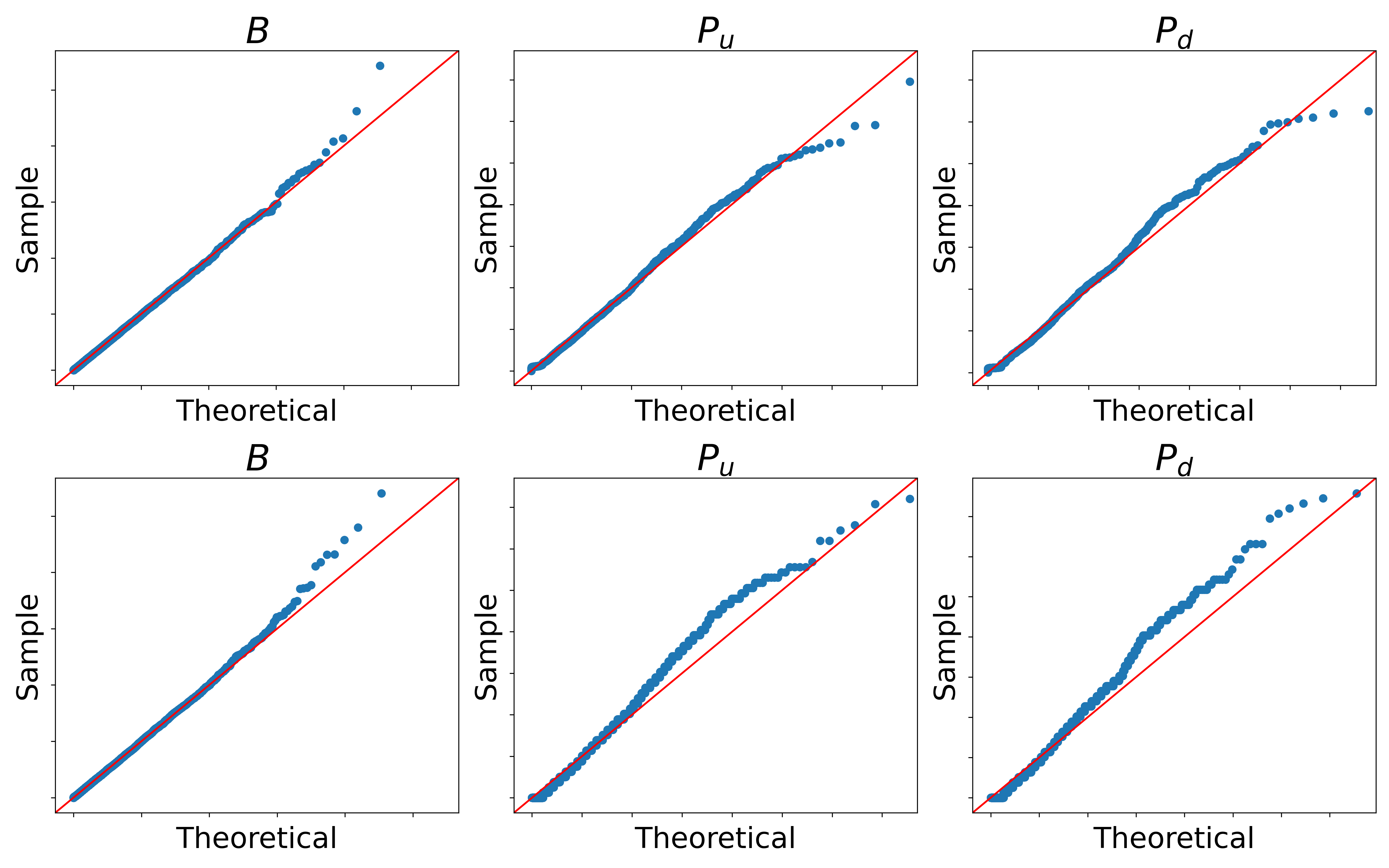
Goodness of Fit test: We test the model’s goodness of fit to determine the appropriateness of the proposed Hawkes processes model for the crypto dataset. According to the random time change theorem[24], if $\{t_{1},\cdots,t_{k}\}$ is a realisation over time $[0,T]$ from a point process with conditional intensity function $\lambda(\cdot)$ , then the transformed points $\{\Lambda(t_{1}),\cdots,\Lambda(t_{k})\}$ form a Poisson process with unit rate. Then the interarrival times $\{\Lambda(t_{1}),\Lambda(t_{2})-\Lambda(t_{1}),\cdots,\Lambda(t_{k})-\Lambda(t_{k-1})\}$ should be independently and identically distributed as exponential random variable with mean $1$ , i.e., $\textrm{exp}(1)$ . Therefore, given a closed form expression of the compensator (12), we can compute the transformed points and use a quantile-quantile plot (Q-Q plot) for exponential distribution to assess the quality of fit.

Fig. 3a shows the Q-Q plot for the Hawkes process fit (upper panel) and the Q-Q plot for a homogeneous Poisson model (lower panel). Fig. 3b compares the deviation of the fitted line’s slope from $45^{\circ}$ . For modeling block arrivals, the Hawkes process model has a slope deviation of 0.002 whereas the Poisson process model has a slope deviation of 0.020; For modeling bitcoin price positive (resp. negative) jumps, the Hawkes process model has a slope deviation of $0.028$ (resp. 0.062) whereas the Poisson process model has a slope deviation of 0.182 (resp. 0.217).

Summary of Results: As seen in entries $(1,2)$ and $(1,3)$ of the kernel norms in Fig. 2, both positive and negative bitcoin price jumps increase the future block mining rate. The off-diagonal entries $(2,3)$ and $(3,2)$ represent mean reversion in bitcoin price returns: positive jumps will result in more negative jumps, while negative jumps will result in more positive jumps.

The smaller slope deviations as shown in Fig. 3b indicate that the Hawkes process model is a better fit to the bitcoin dataset than a Poisson process model.

IV Conclusions

This paper investigated the use of multi-variate Hawkes process to model block arrivals in the bitcoin blockchain. Hawkes processes are self exciting point processes that can capture essential features of blockchain including the self- and cross-exciting impacts of block mining and bitcoin price volatility. The data from the Bitcoin price time series is converted into a sequence of positive and negative price jump events. Maximum likelihood estimation is then used to derive the kernel function for the trivariate Hawkes process. The kernel function norms indicate that price volatility encourages block mining, i.e., both positive and negative price jumps will boost block arrival rate. Using the random time change theorem, we show that the proposed Hawkes process model fits the bitcoin dataset better than a Poisson process model.

Appendix A Block Data Cleaning

All the results shown in Section III are reproducible. The bitcoin price dataset can be downloaded from GitHub⁷⁷ 7 https://github.com/crypto-chassis/cryptochassis-data-api-docs, and the blockchain dataset can be obtained using Google Bigquery⁸⁸ 8 https://cloud.google.com/blog/topics/public-datasets/bitcoin-in-bigquery-blockchain-analytics-on-public-data. We will also make our code public when we submit the paper.

There are two forms of block timestamp errors in the query period, notably duplicated timestamps and out-of-order timestamps. In this section we explain how we clean these erroneous data.

1.

Duplicated timestamps: The first form of error is block timestamp duplication, which occurs when two blocks have the same timestamp. During the time period under consideration, there were two such instances (Fig. 4). One example is that block 719599 and block 719601 both arrived at 2022-01-20 09:26:01, we preserve block 719599 which contains more transactions and remove block 719601 from the dataset.
2.

Out-of-order timestamps: The second form of error involves blocks whose timestamps are earlier than previous blocks. According to [1], out-of-order timestamps are often caused by a miner using a timestamp from the future. In addition, some mining software and mining pools vary the timestamp to use it as an additional nonce in mining. During the query time period, there were 14 such instances (Fig. 5). We re-order the blocks by timestamps.

References

[1] R. Bowden, H. Keeler, A. Krzesinski, and P. Taylor, “Modeling and analysis of block arrival times in the bitcoin blockchain,” Stochastic Models, vol. 36, no. 4, pp. 602–637, 2020.
[2] S. Nakamoto and A. Bitcoin, “A peer-to-peer electronic cash system,” Bitcoin.–URL: https://bitcoin. org/bitcoin. pdf, vol. 4, 2008.
[3] M. Rosenfeld, “Analysis of hashrate-based double spending,” arXiv preprint arXiv:1402.2009, 2014.
[4] Y. Lewenberg, Y. Bachrach, Y. Sompolinsky, A. Zohar, and J. S. Rosenschein, “Bitcoin mining pools: A cooperative game theoretic analysis,” in Proceedings of the 2015 international conference on autonomous agents and multiagent systems. Citeseer, 2015, pp. 919–927.
[5] C. Decker and R. Wattenhofer, “Information propagation in the bitcoin network,” in IEEE P2P 2013 Proceedings. IEEE, 2013, pp. 1–10.
[6] Y. Kawase and S. Kasahara, “Transaction-confirmation time for bitcoin: A queueing analytical approach to blockchain mechanism,” in International Conference on Queueing Theory and Network Applications. Springer, 2017, pp. 75–88.
[7] B. G. Gebraselase, B. E. Helvik, and Y. Jiang, “Transaction characteristics of bitcoin,” in 2021 IFIP/IEEE International Symposium on Integrated Network Management (IM). IEEE, 2021, pp. 544–550.
[8] B. Cao, Z. Zhang, D. Feng, S. Zhang, L. Zhang, M. Peng, and Y. Li, “Performance analysis and comparison of pow, pos and dag based blockchains,” Digital Communications and Networks, vol. 6, no. 4, pp. 480–485, 2020.
[9] P. J. Laub, Y. Lee, and T. Taimre, “The elements of Hawkes processes,” 2022.
[10] E. Bacry, I. Mastromatteo, and J.-F. Muzy, “Hawkes processes in finance,” Market Microstructure and Liquidity, vol. 1, no. 01, p. 1550005, 2015.
[11] A. G. Hawkes, “Spectra of some self-exciting and mutually exciting point processes,” Biometrika, vol. 58, no. 1, pp. 83–90, 1971.
[12] C. G. Bowsher, “Modelling security market events in continuous time: Intensity based, multivariate point process models,” Journal of Econometrics, vol. 141, no. 2, pp. 876–912, 2007.
[13] V. Filimonov and D. Sornette, “Quantifying reflexivity in financial markets: Toward a prediction of flash crashes,” Physical Review E, vol. 85, no. 5, p. 056108, 2012.
[14] R. C. Phillips and D. Gorse, “Mutual-excitation of cryptocurrency market returns and social media topics,” in Proceedings of the 4th international conference on frontiers of educational technologies, 2018, pp. 80–86.
[15] N. Du, M. Farajtabar, A. Ahmed, A. J. Smola, and L. Song, “Dirichlet-hawkes processes with applications to clustering continuous-time document streams,” in Proceedings of the 21th ACM SIGKDD international conference on knowledge discovery and data mining, 2015, pp. 219–228.
[16] E. Choi, N. Du, R. Chen, L. Song, and J. Sun, “Constructing disease network and temporal progression model via context-sensitive hawkes process,” in 2015 IEEE International Conference on Data Mining. IEEE, 2015, pp. 721–726.
[17] P. Zheng, S. Yuan, and X. Wu, “Using dirichlet marked hawkes processes for insider threat detection,” Digital Threats: Research and Practice (DTRAP), vol. 3, no. 1, pp. 1–19, 2021.
[18] S. J. Hardiman, N. Bercot, and J.-P. Bouchaud, “Critical reflexivity in financial markets: a Hawkes process analysis,” The European Physical Journal B, vol. 86, no. 10, pp. 1–9, 2013.
[19] T. J. Liniger, “Multivariate Hawkes processes,” Ph.D. dissertation, ETH Zurich, 2009.
[20] A. Verma, S. G. Jena, D. R. Isakov, K. Aoki, J. E. Toettcher, and B. E. Engelhardt, “A self-exciting point process to study multicellular spatial signaling patterns,” Proceedings of the National Academy of Sciences, vol. 118, no. 32, 2021.
[21] F. P. Schoenberg, “Introduction to point processes,” Wiley Encyclopedia of Operations Research and Management Science, 2010.
[22] M. Dresher, The mathematics of games of strategy. Courier Corporation, 2012.
[23] M. Mark, J. Sila, and T. A. Weber, “Quantifying endogeneity of cryptocurrency markets,” The European Journal of Finance, pp. 1–16, 2020.
[24] D. J. Daley, D. Vere-Jones et al., An introduction to the theory of point processes: volume I: elementary theory and methods. Springer, 2003.
[25] M. Bompaire, “Machine learning based on Hawkes processes and stochastic optimization,” Ph.D. dissertation, Université Paris Saclay (COmUE), 2019.
[26] A. Veen and F. P. Schoenberg, “Estimation of space–time branching process models in seismology using an em–type algorithm,” Journal of the American Statistical Association, vol. 103, no. 482, pp. 614–624, 2008.
[27] G. Cloud, “Bitcoin in bigquery: blockchain analytics on public data,” https://cloud.google.com/blog/topics/public-datasets/bitcoin-in-bigquery-blockchain-analytics-on-public-data, 2022.
[28] C. Chassis, “Public data api from cryptochassis,” https://github.com/crypto-chassis/cryptochassis-data-api-docs, 2022.
[29] S. Y. Yang, A. Liu, J. Chen, and A. Hawkes, “Applications of a multivariate Hawkes process to joint modeling of sentiment and market return events,” Quantitative finance, vol. 18, no. 2, pp. 295–310, 2018.
[30] P. Embrechts, T. Liniger, and L. Lin, “Multivariate Hawkes processes: an application to financial data,” Journal of Applied Probability, vol. 48, no. A, pp. 367–378, 2011.
[31] M. Mudassir, S. Bennbaia, D. Unal, and M. Hammoudeh, “Time-series forecasting of bitcoin prices using high-dimensional features: a machine learning approach,” Neural computing and applications, pp. 1–15, 2020.
[32] E. Bacry, M. Bompaire, S. Gaïffas, and S. Poulsen, “Tick: a python library for statistical learning, with a particular emphasis on time-dependent modelling,” arXiv preprint arXiv:1707.03003, 2017.
[33] E. Bacry, T. Jaisson, and J.-F. Muzy, “Estimation of slowly decreasing Hawkes kernels: application to high-frequency order book dynamics,” Quantitative Finance, vol. 16, no. 8, pp. 1179–1201, 2016.