Distributed Optimization of Average Consensus Containment with Multiple Stationary Leaders

The idea of achieving a common objective in a system with multiple agents using distributed and co-operative control has garnered a lot of interest among research community for a long time. A fundamental aspect of the distributed co-operative control is that the agents achieve the collective objective via local interaction among neighbours, thereby making the framework robust to communication failures, highly adaptable and cost effective.

A well addressed problem in this multi-agent system framework is the consensus problem, where the agents are expected to agree on a common value [15], [13]. Consensus with a single leader is addressed in [4]. When there are multiple leaders the problem is referred to as containment control where the objective is to bring the remaining follower agents from any arbitrary state, within the convex hull spanned by the leaders’ state [20]. This problem is also motivated from nature such as gravel ants forming a boundary over caterpillars and transporting along with them due to their sugary extract. Practical applications include shaping of social dynamics using a set of guiding agents, military applications, safe disposal of hazardous waste etc. [2]. Extensive research is done in this area such as analysing dynamic leaders using PDE in [5], assuming directed static topology [9], time-varying topologies [1], agents with higher order dynamics and impact of time delays [8].

While the above containment algorithms only focus on general containment of followers, i.e. each follower achieving an arbitrary state, different from each other, within the convex hull of the leaders, the primary objective of this paper is to achieve a consensus among the followers regarding the final destination within the convex hull of the leaders. The idea of achieving consensus in a multiple leader containment scenario is motivated by various applications. One is opinion consensus of a group, driven by a couple of external agents/factors, in a direction that gets aligned with their own priors. Another application is a cooperative attack on a static or, moving target, where the target is encircled by UAVs (leaders) such that the target’s live location coincides with the average of coordinates of UAVs. Then the missiles (followers) can easily home in to the target without the need for any individual radar tracking.

Motivated by the above applications for consensus containment, we provide an algorithm where the followers reach a consensus to the average of the leaders’ state. [7] investigates consensus of followers inside the convex hull of stationary leaders, where a distributed control law has been designed by formulating a centralized multi-objective optimization (MOP) with a trade-off between performance error and convergence rate. This results in a significant asymptotic drift in the final consensus value due to non-convergence to the exact solution on account of trade-offs. We propose a distributed control law which ensures a fast convergence of the followers to the consensus within the convex hull spanned by the leaders over a directed network, without any aforementioned asymptotic drift. The fast convergence is designed using a distributed optimization algorithm unlike the centralized approach in [7]. Distributed optimization of convergence rate to consensus without leaders in a multi-agent, undirected framework is addressed in [18].

We summarize our contribution as follows.

1. 1.

   We consider a multi-agent system with multiple stationary leaders and followers communicating with each other over a directed network topology. We propose a distributed algorithm which ensures consensus of followers to the average of leaders’ states.

2. 2.

   We formulate an optimization problem to maximize the rate of convergence of follower agents to the consensus value. We propose an algorithm based on Alternating Direction Method of Multipliers (ADMM) that solves the above optimization problem in a distributed manner.

3. 3.

   We illustrate the results using numerical examples. We compare the results of the distributed optimization to the centralized optimization.

The outline of the paper is laid out as follows. Following the introduction, Section II focuses on basic mathematical preliminaries. In Section III, the two problems are formally discussed. Algorithms for solving these problems are proposed in Section IV. Section V provides a numerical example to elucidate the validity of the proposed algorithms. Finally, we give concluding remarks in Section VI. The proofs of some of the results are in Appendix.

In this section, we briefly introduce some preliminaries pertaining to directed graphs and convex analysis.

We first explain the framework of a multi-agent system with more than one leader. Consider a group of $n$ agents communicating with each other. The communication pattern is depicted by a directed graph $\mathcal{G}$. The vertices of the graph correspond to the agents and the state of an agent $j$ is accessible by agent $i$ only if there is a directed edge $(v_{j},v_{i})$ in the graph. An agent is designated to be a leader if its in-neighbour set is empty. The rest of the agents are termed as followers. Let $\mathcal{L}$ and $\mathcal{F}$ denote respectively the index set of leaders and followers. Let $\mathcal{G^{F}}$ be the subgraph induced by the vertex set of the followers, $v_{i}\ \forall\ i\in\mathcal{F}$ and $\mathcal{G^{FL}}$ is a subgraph with vertex set $\mathcal{V}$ and edge set given by $\mathcal{E^{FL}}=\big\{(v_{j},v_{i})\in\mathcal{E}\ \forall\ i\in\mathcal{F},\ j\in\mathcal{L}\big\}$. Let $x_{i}\in\mathbb{R}$ denote the state of each agent and assume that they follow the following discrete time dynamics.

where $u_{i}(k)$ is the control input to agent $i$ at $k^{th}$ iteration. The following are our assumptions on the agents.

In this section, we present a numerical example that illustrates our result when all the agents are in 2-D plane.

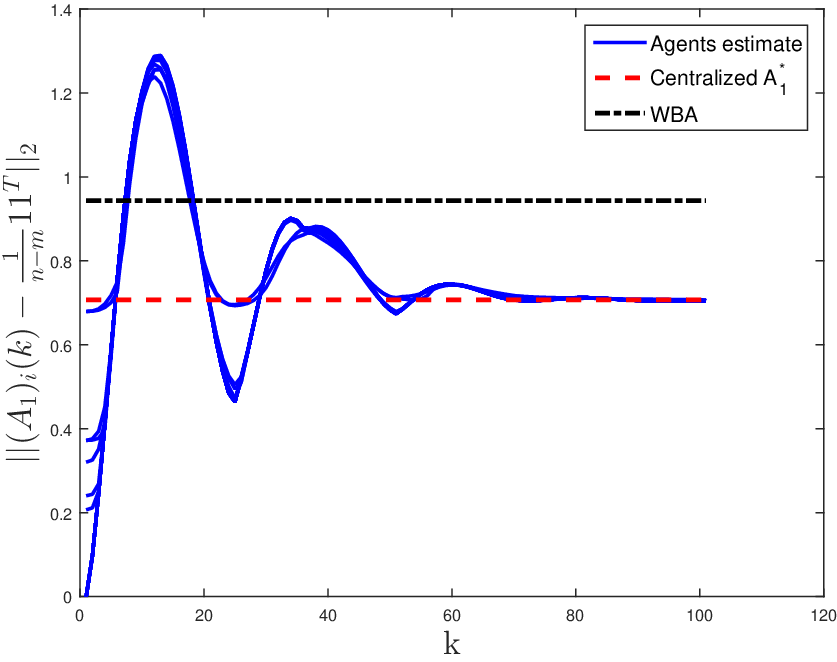
We consider a set of 24 agents interacting over a directed network topology, i.e., $n=24$. Assume that there are $m=10$ leaders, and the rest are followers interacting as shown in Fig. 1. Let $x^{1}$ and $x^{2}$ denote two sets of state variable that indicates the position of each agent in 2-D plane. The state values of the stationary leader agents are given by $x^{1}_{L}=$[5 3 2 2 3 5 7 8 8 7]^T and $x^{2}_{L}=$[1 2 4 5 7 8 7 5 4 2]^T. Algorithm 2 is employed to compute an optimal $A_{1}$ matrix in a distributed manner. Then using that $A_{1}$ and any random choice of $A_{2}$ following Assumption 1, Algorithm 1 is employed to ensure that follower agents reach a consensus to the average of the stationary leader states which is $(\bar{x}^{1}_{L},\bar{x}^{2}_{L})=(5,4.5)$, is illustrated in Fig. 2.

The convergence factors of the weight matrices $(A_{1})$ generated by different methods have been given in Table I, for comparison purposes. A weight-balance algorithm (WBA) proposed in [10] generates balancing weights for a directed network, which, although not optimal, is computed in a distributed manner.

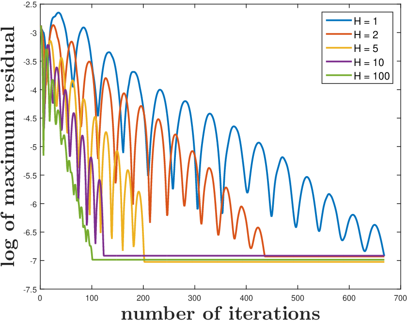
It can be observed that $A_{1}$ computed by Algorithm 2 is quite close to the optimal $A_{1}^{*}$ given by centralized methods as depicted in Fig. 3, and performs much better than that of WBA. In Remark 3, we explained how the performance of Algorithm 2 improves with increase in $H$. This is illustrated in Fig. 4 where we observe that the residual values decreases faster for increase in values of $H$.

We considered a special case of the discrete-time containment control problem for multi-agent systems with multiple stationary leaders, interacting over a directed communication topology. We studied the problem of achieving faster convergence to a consensus among followers to the average of the leaders’ state, terming it as the average consensus containment. First, we provided sufficient conditions that guarantee average consensus containment. A distributed algorithm was proposed that ensured average consensus containment. Using this analysis, an optimization problem was formulated to maximize the convergence rate which was also solved in a distributed manner using ADMM algorithm. Through numerical examples, we demonstrated that the optimal convergence rate obtained using locally computed weights in a distributed manner is very close to the optimal value obtained by centralized methods. Moving forward, it would be interesting to investigate analogous results using dynamic leaders, and under a continuous-time setting.

Since $A_{1}$ is a column stochastic matrix associated with a strongly-connected graph (Assumption 1), it is irreducible [3]. Furthermore, [11, Sec. 8.3], $A_{1}$ is primitive as its non-negative irreducible with positive diagonal entries due to each follower knowing its own state. Hence, $1$ is a simple eigenvalue of $A_{1}$. Let $u_{r}$ and $u_{l}$ respectively denote the right and left eigenvector of $A_{1}$ corresponding to eigenvalue $1$. Note that $u_{l}=\frac{1_{n-m}}{\sqrt{n-m}}$. Using [11, Sec 7.10] we get

where, $G$ is the spectral projector onto nullspace of $(I_{n-m}-A_{1})$ along the columnspace of $(I_{n-m}-A_{1})$, and is given by $G=u_{r}u_{l}^{T}$. Also, as per [11, Sec 8.4], $A_{1}$ being column-stochastic, is Cesáro summable, with the Cesáro limit

From (10), (11),

In Algorithm 1, from Step 3 we get $x_{i}(k)=\frac{\left[s(k)\right]_{i}}{\left[w(k)\right]_{i}}$ which when using the update law $\forall\ i\in\mathcal{F}$, becomes
$x_{i}(k)=\frac{\left[A_{1}^{k}x_{F}(0)+\{A_{1}^{k-1}+A_{1}^{k-2}+...+A_{1}+I_{n-m}\}A_{2}x_{L}(0)\right]_{i}}{\left[A_{1}^{k}1_{n-m}+\{A_{1}^{k-1}+A_{1}^{k-2}+...+A_{1}+I_{n-m}\}A_{2}1_{m}\right]_{i}}$

Dividing numerator and denominator by $k$ and taking limits with $x_{i}^{s}:=\underset{k\rightarrow\infty}{\lim}x_{i}(k)$.
$x_{i}^{s}=\frac{\left[\underset{k\rightarrow\infty}{\lim}\frac{A_{1}^{k}x_{F}(0)}{k}+\underset{k\rightarrow\infty}{\lim}\big\{\frac{A_{1}^{k-1}+A_{1}^{k-2}+...+A_{1}+I_{n-m}}{k}\big\}A_{2}x_{L}(0)\right]_{i}}{\left[\underset{k\rightarrow\infty}{\lim}\frac{A_{1}^{k}1_{n-m}}{k}+\underset{k\rightarrow\infty}{\lim}\big\{\frac{A_{1}^{k-1}+A_{1}^{k-2}+...+A_{1}+I_{n-m}}{k}\big\}A_{2}1_{m}\right]_{i}}$
From (10), $\left[\underset{k\rightarrow\infty}{\lim}\frac{A_{1}^{k}x_{F}(0)}{k}\right]_{i}\rightarrow 0$ and $\left[\underset{k\rightarrow\infty}{\lim}\frac{A_{1}^{k}1_{n-m}}{k}\right]_{i}\rightarrow 0$.
From (10), (12), we get

Since, $A_{2}$ is column stochastic, $1_{n-m}^{T}A_{2}=1_{m}^{T}$. Hence,

From the above equation, we observe that the followers are in consensus at the average of the leaders’ state values. Hence the proof.∎

From (13) we have $\quad\forall\ i\in\mathcal{F}$,

$A_{1}$ is primitive and as such, its eigenvalues satisfy $\lambda_{1}=1>\lambda_{2}\geq\ldots\geq\lambda_{n-m}$. Therefore, the convergence rate of $x_{i}(k)$ is determined by $\lambda_{2}=\rho\big(A_{1}-\frac{1}{n-m}\mathbf{11}^{T}\big)$.∎

The augmented Lagrangian ($L_{\rho}$) for (IV-B) is given by

where $\rho>0$ is the penalty parameter. Now, the standard 2-block ADMM algorithm for (IV-B) is given below. The primal variables $\big[(A_{1})_{i}(k)\ \forall\ i\in\mathcal{F},\ Z(k)\big]$ are updated sequentially and dual variables $\big[C_{i}(k)\ \forall\ i\in\mathcal{F}\big]$ are updated afterwards. The constraint set $S:=\big\{(A_{1})_{i}\ |\ (A_{1})_{i}\mathbf{1}=\mathbf{1},\ (A_{1})_{i}^{T}\mathbf{1}=\mathbf{1},\ (A_{1})_{i}^{ij}=0,\ (i,j)\notin\mathcal{E^{\mathcal{F}}}\big\}$ has been incorporated into primal update steps rather than being dualized.
$Z$ update step : $Z(k+1)=\underset{Z}{argmin}\big\{L_{\rho}\big\}$

The $Z$ update step involves computing an average across all follower agents over a directed network. Hence we use an approach based on dynamic average consensus, proposed in [17], to get the $Z$ update step, in a distributed manner. Each agent $i\in\mathcal{F}$ maintains $Z_{i}$ which is an estimate for $Z$. Before we provide a distributed update law for $Z$, we write the update law for the other variables.
$(A_{1})_{i}$ update step : $(A_{1})_{i}(k+1)=\underset{S}{argmin}\{L_{\rho}\}$

$C_{i}$ update step :

Note that in both (17) and (18), we use the estimate $Z_{i}$ instead of $Z$. Next, we simplify the $Z$ update step in (16). At every iteration $k$, each agent initializes a variable $M_{i}(0,k):=Z_{i}(k)+(A_{1})_{i}(k+1)-(A_{1})_{i}(k)+\frac{C_{i}(k)-C_{i}(k-1)}{\rho}$. From (18), this is further simplified as $M_{i}(0,k)=(A_{1})_{i}(k+1)$. For some $H\geq 1$, $0\leq t\leq H-1$, $i\in\mathcal{F}$ do

Then $Z_{i}(k+1)=M_{i}(H,k)$. In (19), $d_{i}:=|\mathcal{N}^{out}_{i}|$ is the out-degree of $i^{th}$ follower agent. In (20), $v_{i}(t,k)\in\mathbb{R}$ is the node-weight used by $i^{th}$ agent to scale its outgoing information and evolves dynamically as shown. As defined in [10], the node-weights are initialized as $v_{i}(0,0)\leq(1/d^{*})^{2D+1}$, where $D$ is the diameter of the subgraph $\mathcal{G^{F}}$ and $d^{*}=\underset{i\in\mathcal{F}}{max}\ d_{i}$. Each of the agent $i\in\mathcal{F}$ initialises a small value as its node-weight, $v_{i}(0,0)>0$.∎

References

- [1] Yongcan Cao and Wei Ren. Containment control with multiple stationary or dynamic leaders under a directed interaction graph. In Proceedings of the 48h IEEE Conference on Decision and Control (CDC), pages 3014–3019. IEEE, 2009.
- [2] Yongcan Cao, Daniel Stuart, Wei Ren, and Ziyang Meng. Distributed containment control for multiple autonomous vehicles with double-integrator dynamics: algorithms and experiments. IEEE Transactions on Control Systems Technology, 19(4):929–938, 2010.
- [3] Jiu Ding and Noah H Rhee. On the equality of algebraic and geometric multiplicities of matrix eigenvalues. Applied Mathematics Letters, 24(12):2211–2215, 2011.
- [4] Ali Jadbabaie, Jie Lin, and A Stephen Morse. Coordination of groups of mobile autonomous agents using nearest neighbor rules. IEEE Transactions on Automatic Control, 48(6):988–1001, 2003.
- [5] Meng Ji, Giancarlo Ferrari-Trecate, Magnus Egerstedt, and Annalisa Buffa. Containment control in mobile networks. IEEE Transactions on Automatic Control, 53(8):1972–1975, 2008.
- [6] David Kempe, Alin Dobra, and Johannes Gehrke. Gossip-based computation of aggregate information. In 44th Annual IEEE Symposium on Foundations of Computer Science, 2003. Proceedings., pages 482–491. IEEE, 2003.
- [7] Usman A Khan, Soummya Kar, and José MF Moura. Higher dimensional consensus: Learning in large-scale networks. IEEE Transactions on Signal Processing, 58(5):2836–2849, 2010.
- [8] Bo Li, Hong-Yong Yang, Zeng-Qiang Chen, and Zhong-Xin Liu. Distributed containment control of multi-agent systems with general linear dynamics and time-delays. International Journal of Control, Automation and Systems, 16(6):2718–2726, 2018.
- [9] Huiyang Liu, Guangming Xie, and Long Wang. Necessary and sufficient conditions for containment control of networked multi-agent systems. Automatica, 48(7):1415–1422, 2012.
- [10] Ali Makhdoumi and Asuman Ozdaglar. Graph balancing for distributed subgradient methods over directed graphs. In 2015 54th IEEE Conference on Decision and Control (CDC), pages 1364–1371. IEEE, 2015.
- [11] Carl D Meyer. Matrix Analysis and Applied Linear Algebra, volume 71. Siam, 2000.
- [12] Giuseppe Notarstefano, Ivano Notarnicola, and Andrea Camisa. Distributed optimization for smart cyber-physical networks. arXiv preprint arXiv:1906.10760, 2019.
- [13] Reza Olfati-Saber, J Alex Fax, and Richard M Murray. Consensus and cooperation in networked multi-agent systems. Proceedings of the IEEE, 95(1):215–233, 2007.
- [14] Michael L Overton and Robert S Womersley. On minimizing the special radius of a nonsymmetric matrix function: Optimality conditions and duality theory. SIAM Journal on Matrix Analysis and Applications, 9(4):473–498, 1988.
- [15] Wei Ren and Randal W Beard. Consensus seeking in multiagent systems under dynamically changing interaction topologies. IEEE Transactions on Automatic Control, 50(5):655–661, 2005.
- [16] R Tyrrell Rockafellar. Convex analysis, volume 36. Princeton university press, 1997.
- [17] Kiran Rokade and Rachel Kalpana Kalaimani. Distributed admm over directed graphs. arXiv preprint arXiv:2010.10421, 2020.
- [18] Kiran Rokade and Rachel Kalpana Kalaimani. Distributed computation of optimal weights for consensus using admm. arXiv preprint arXiv:2002.08106, 2020.
- [19] Dong Wang and Wei Wang. Necessary and sufficient conditions for containment control of multi-agent systems with time delay. Automatica, 103:418–423, 2019.
- [20] Feng Xiao and Long Wang. Consensus behavior of agents in networked systems under general communication topologies. In 2006 IEEE Conference on Computer Aided Control System Design, pages 862–867. IEEE, 2006.
Appendix
Proof of Theorem 1
Since is a column stochastic matrix associated with a strongly-connected graph (Assumption 1), it is irreducible [3]. Furthermore, [11, Sec. 8.3], is primitive as its non-negative irreducible with positive diagonal entries due to each follower knowing its own state. Hence, is a simple eigenvalue of . Let and respectively denote the right and left eigenvector of corresponding to eigenvalue . Note that . Using [11, Sec 7.10] we get