Instanton effects in Euclidean vacuum,
real time production and in the light front wave functionsPresented at 2021 Zakopane school
Abstract
Nontrivial topological structures of non-Abelian gauge fields were discovered in the 1970’s. Instanton solutions, describing vacuum tunneling through topological barriers, have fermionic zero modes which are at the origin of ′t Hooft effective Lagrangian. In the 1980’s instanton ensembles have been used to explain chiral symmetry breaking. In the 1990’s a large set of numerical simulations were performed deriving Euclidean correlation functions. The special role of scalar diquarks in nucleons, and color superconductivity in dense quark matter have been elucidated.
In these lectures, we discuss further developments of physics related to gauge topology. We show that the instanton-antiinstanton “streamline” configurations describe “sphaleron transitions” in high energy collisions, which result in production of hadronic clusters with nontrivial topological/chiral charges. (They are not yet observed, but discussions of dedicated experiments at LHC and RHIC are ongoing.)
Another new direction is instanton effects in hadronic spectroscopy, both in the rest frame and on the light front. We will discuss their role in central and spin-dependent potentials, formfactors and antiquark nuclear “sea”. Finally, we summarize the advances in the semiclassical theory of deconfinement, and chiral phase transitions at finite temperature, in QCD and in some of its “deformed” versions.
PACS numbers come here
1 Brief overview of gauge topology
We start these lectures with a map, outlining the role and interdependence of various topological structures in the QCD vacuum. The phenomenon of color confinement (left blue region in Fig.1) was first related with center vortices, associated with a phase for a quark looping around, changing the sign of the linking Wilson line. Two such vortices combined together, lead to a singularity with a phase , shown by white an arrow, known as the Dirac string. Their ends are identified as magnetic monopoles (blue disks). Confinement is their Bose-Einstein condensation, perhaps the most physical signature of this phenomenon.
The right yellow region of Fig.1 is associated with another major nonperturbative phenomenon, chiral symmetry breaking. The pink disk refers to instantons, 4D solitons in Euclidean space-time. Fermions in this field have zero modes, elevating each instanton into ′t Hooft multi-fermion operator. The four black arrows correspond to the case of two quark flavors, . The resulting 4-fermion vertex is similar to Nambu-Jona-Lasinio hypothetical interaction, and also breaks spontanously chiral symmetry provided the instanton density is sufficiently large.
At finite temperature the Polyakov line has a number of eigenvalues or (see below). The instanton solution amended by such asymptotics for the field, splits into instanton constituents, known as instanton-dyons or instanton-monopoles11 1 Both names were criticized: they are neither the dyons of Schwinger, nor monopoles of Dirac, but Euclidean self-dual objects, with equal and up to a sign. Perhaps a new name, emphasizing their Euclidean nature, is needed: can it e.g. be ? . Like instantons, they have topological charges. Unlike instantons, the charges are not quantized to integers . This is possible since they are connected by Dirac strings due to their magnetic charges. Ensembles of these topological objects will be shown to generate both confinement, and chiral breaking at the end of these lectures.
Last but not least is the phenomenon of Poisson duality, started as a technical observation relating partition functions derived in terms of monopoles and in terms of instanton-dyons. As we will discuss below, it has wider meaning: their equality brings to mind equivalence of two other great approaches to classical dynamics, by Hamilton and Lagrange, respectively.
The detailed discussion of these configurations, in addition to discussions about the QCD flux tubes and holographic QCD etc, can be found in [1].
2 Brief history of instantons
2.1 Semiclassical theory based on path integrals: instantons and fluctons
The quantum mechanics courses include semiclassical methods based on certain representation of the wave function, starting with the celebrated Bohr-Sommerfeld quantization condition, applied to the oscillator and hydrogen atom, and followed by Wentzel-Kramers-Brillouin (WKB) approximation, developed in 1926. Unfortunately, subsequent study has shown that generalization of those to physical systems with more than one degree of freedom, as well as to systematic order-by-order account for quantum fluctuations, are not possible.
By definition the Feynman path integral gives the density matrix in coordinate representation (see e.g. a very pedagogical Feynman-Hibbs book)
| (1) |
Note that it is a function of the initial and final coordinates, as well as the time needed for the transition. Here is the classical action of the system, e.g. for a particle of mass in a static potential it is
Feynman has shown that the oscillating exponent along the path, provides the correct weight of the paths integral (1). For reference, the same object can also be written in a form closer to that used in quantum mechanics courses. Heisenberg wrote it as a matrix element of the time evolution operator, the exponential of the Hamiltonian 22 2 Here, we assume that the motion happens in a time-independent potential, for otherwise the exponential is time ordered.
| (2) |
between states in which a particle is localized in-out.
Schroedinger set of stationary states can also be used as a basis set. Because the Hamiltonian is diagonal in this basis, there is a single (not double) sum
| (3) |
with . Oscillating weights for different states are often hard to calculate, and one may wonder if it is possible to analytically continue in time, to the Euclidean version with absorbed into it. For reasons which will soon become clear, we will also define this imaginary time on a circle with circumference
In this way we will be able to describe mechanics of a particle in a heat bath with temperature related to the circle circumference
Such periodic time is known as the Matsubara time. The expression (3) is now
| (4) |
which sums the quantum-mechanical probabilities to find a particle at point , times its thermal weight. Performing the integral over all , and using the normalization of the weight functions, one finds the expression for the thermal partition function
| (5) |
We will use this expression below in a Feynman path integral form, with (i) taken over all paths with the same endpoints, and with (ii) Euclidean or rotated time. The probability to find a particle at a certain point is then
| (6) |
Note that here, the exponent is not oscillating and equals the Euclidean action
| (7) |
in which the sign of the potential is reversed, and the time derivative is understood to be over .
Looking for the periodic paths with the minimal action, one may start with the simplest, i.e. a particle at rest with ! Such path is dominant for small time (Matsubara circle), with (or high temperature )33 3 Note that it is opposite to the limit discussed above in the Hamiltonian approach. If one ignores the time dependence and velocity on the paths, there is no kinetic term and only the potential one in the action contributes. So
| (8) |
which corresponds to classical44 4 Note that if we would keep , the one in and in the exponent would cancel out, confirming the classical nature of this limit. thermal distribution for a particle in a potential .
Since the weight is , the paths with the smallest action should give the largest contribution. These paths satisfy the classical (Euclidean) equation of motion, as we will carry below. The semiclassical approximation – the of these paths – would be justified, as soon as the corresponding action is large
| (9) |
Such classical paths were called fluctons in [2]. These paths should have Euclidean time period . For simplicity, let us start with “cold” QM, or vanishingly small , . Little thinking of how to arrange a classical path with a very long period leads to the following solution: the particle should roll to the top of the (flipped) potential with exactly such energy as to sit there for very long time, before it will roll back to the (arbitrary) point from which the path started. The classical paths corresponding to relaxation toward the potential bottom take the form of a path “climbing up” from an arbitrary point to the maximum, see Fig. 2

Let us start with the harmonic oscillator, as the unavoidable first example. For simplicity, let us use the canonical units, in which the particle mass is , and the oscillator frequency is , so that our (Euclidean) Lagrangian 55 5 Note again the flipped sign of the potential term. In Minkowski time the potential has sign minus. is simplified to
| (10) |
Because of this sign, in Euclidean time the oscillator does not oscillate but relaxes . For a harmonic oscillator, the classical equations of motion (EOM) are of course not difficult to solve. However, it is always easier to get solutions using energy conservation (first integral of motion for static potentials). Since we are interested in solutions with zero energy , they correspond to . The boundary conditions are , at plus periodicity on a circle with circumference . This solution is
| (11) |
defined for . The particle moves toward and reaches some minimal value, at , and then returns to the initial point again at . Due to the periodicity in , one may shift its range to . The minimal value at
is exponentially small at low temperature. The climbing to the potential top at is nearly accomplished, if the period is large.
The solution in the zero temperature or limit simplifies to . In the opposite limit of small or high , there is no time to move far from , so in this case the particle does not move at all. The classical action of the flucton path is
| (12) |
The result means that the particle distribution
| (13) |
is Gaussian at any temperature. Note that the width of the distribution
| (14) |
is the ground state energy plus the contribution due to the thermal excitations, which we already mentioned at the beginning of the chapter. So, the flucton reproduces the well known results for the harmonic oscillator, see e.g. Feynman’s Statistical Mechanics.
Flucton solutions for several well used QM problems (anharmonic oscillator, the quartic double well, sin-like potential) were discussed in detail in [12]. Unlike WKB, one can define and calculate semiclassical series in by well-defined procedure, using Feynman diagrams. Finite temperature fluctons were used for anharmonic oscillator and 4-nucleon clustering in [11].
Quantum mechanical instantons were introduced66 6 It is interesting that the first application to the QFT problem – pairs production in constant electric field – were done already in 1931, by Sauter [3] . by [4] in the context of tunneling in the double-well potential. In the inverted potential it is a path going from one maximum to another.
For an early pedagogical review, including the one-loop (determinant) calculation by the same tedious scattering-phase method see ABC’s of instantons [5]. Two-loop corrections were first calculated in [6], some technical errors in it were corrected by Shuryak and Wohler in [7]. Three loop corrections have been calculated by Escobar-Ruiz, Turbiner and Shuryak in [8].
The calculation goes in the same standard way, the path is written as a classical plus quantum fluctuation , and then the action is expanded in powers of . One technical (but important) difference between the and , is that in the former case the fluctuation operator () has a zero mode, related to time-shift symmetry. Therefore the Green function for the fluctuations, needs to be defined in a nonzero mode subspace of Hilbert space. This complication leads to new features, such as additional diagrams not following directly from the Lagrangian.
The Gauge theory instanton was found in the famous work by Belavin, Polyakov, Schwartz and Tyupkin, and since known as the BPST instanton [9]. Let us recall how it was obtained, as some of the expressions will be useful for later use. To find the classical solution corresponding to tunneling, BPST used the following 4-dimensional spherical ansatz depending on the trial function
| (15) |
with and the ’t Hooft symbol defined by
We also define by changing the sign of the last two equations. Upon substitution of the gauge fields in the gauge Lagrangian one finds that the effective Lagrangian has the form
| (20) |
corresponding to the motion of a particle in a double-well potential. The Euclidean solution is that of a quantum mechanical instanton, connecting the of the flipped potential. The corresponding field is
| (21) |
Here is an arbitrary parameter characterizing the size of the instanton. Like in the potential we discussed in the preceding section, its appearance is dictated by the scale invariance of the classical Yang-Mills equation. The ansatz itself perhaps needs some explanation. The ’t Hooft symbol projects to sefl-dual fields, which best captured by the identity
| (22) |
where is the dual field strength tensor (the field tensor in which the roles of electric and magnetic fields are interchanged). Since the first term is a topological invariant (see below) and the last term is always positive, it is clear that the action is minimal if the field is (anti)self-dual77 7 This condition is written in Euclidean space. In Minkowski space there is an extra in the electric field.
| (23) |
In a simpler language, it means that the Euclidean electric and magnetic fields are the same88 8 In the BPST paper the self-duality condition (1-st order differential equation) was solved, rather than (2-nd order) EOM for the quartic oscillator. . The action density is given by
| (24) |
It is spherically symmetric, and very well localized, at large distances it is . The action depends on the scale only via the running coupling
| (25) |
The one-loop (determinant) quantum corrections were calculated in the classic paper by ′t Hooft [10]. The two-loop and higher order quantum corrections have not been calculated to this day, due to the difficulties with the part of the Green functions related to the nonzero modes.
2.2 Chiral symmetry breaking in QCD
Chiral symmetries are additional symmetries that appear when quarks are massless. Since the mass term is the only one in the QCD Lagrangian connecting spinors with right (R) and left (L) chiralities, the symmetry of flavor quark rotations, gets doubled by acting on the L- and R-quarks separately. Also, it can be viewed as and transformations, in which rotations on the L- and R-spinors in the same or opposite directions. The latters are further split into (acting on all quarks by and .
The physics of the nonperturbative vacuum of strong interaction started even before QCD. Nambu and Jona-Lasinio (NJL) [13], inspired by BCS theory of superconductivity, have qualitatively explained that strong enough attraction of quarks can break chiral symmetry spontaneously and, among many other effects, create near-massless pions.
Instantons, the basis for a semiclassical theory of the QCD vacuum and hadrons, has been discovered in 1970’s [9], and soon ′t Hooft has found their fermionic zero modes and formulated his famous effective Lagrangian [10]. Not only it solved the famous “ problem” – by making the non-Goldstone and heavy – but it also produces a strong attraction in the and channels. In the framework of the so called instanton liquid model (ILM) [14], it provided a microscopic (QCD-based) basis for chiral symmetry breaking, chiral perturbation theory and the pion properties. Its two parameters
| (26) |
play the same role as the cutoff and coupling in the NJL model. These parameters have withstood the scrutiny of time, and describe rather well the chiral dynamics related to pions, the Euclidean correlation functions in the few femtometers range, interacting ensemble of instantons, and much more, see [15] for a review.
The subject of these lectures is many other uses of instantons discussed in recent works. We will consider quark pair production, and its role in the isospin asymmetry of the nucleon “sea”, the inclusion of molecules in mesonic formfactors, and forces between quarks in hadrons.
2.3 Euclidean correlation functions
This analysis originally started from the small-distance OPE and the QCD sum rule method, it moved to intermediate distances (see review e.g. in [16]),
First, the experimentally known correlation functions were reproduced by the instanton liquid model at small distances at a quantitative level. Then, for many mesonic channels [18, 19], significant numerical efforts were made, allowing to calculate the relevant correlation functions till larger distances (of about 1.5 fm), where they decay by few decades. As a result, the predictive power of the model has been explored in substantial depth. Many of the coupling constants and even hadronic masses were calculated, with good agreement with experiment and lattice.
2.4 Diquarks and color superconductivity
Subsequent calculations of baryonic correlators [20] has revealed further surprising facts. In the instanton vacuum the nucleon was shown to be made of a “constituent quark” plus a deeply bound , with a mass nearly the same as that of constituent quarks. On the other hand, decuplet baryons (like ) had shown no such diquarks, remaining weakly bound set of three constituent quarks. Deepling bound scalar diquarks are a direct consequence of the ’t Hooft Lagrangian, a mechanism that is also shared by the Nambu-Jona-Lasinio interaction [21], but ignored for a long time.
It also leads to the realization that diquarks can become Cooper pairs in dense quark matter, see [22] for a review on “color superconductivity”.
3 The topological landscape and sphaleron production processes
There has been significant development in the understanding of the “topological landscape” in relation between instantons and sphaleron production processes, see [23]. Recently there have been renewed interest, due to the possible experimental searches for sphaleron production at RHIC/LHC [24]. The sphalerons are 3-dimensional, static and purely magnetic configurations, that minimize the energy functional. To quantify them, we will focus on two main variables. Their topological Chern-Simons number, and their squared field size
| (27) |
If those are kept constant, by adding pertinent Lagrange multipliers to the action, we can find the energy and Chern-Simons number in parametric form
| (28) |
where corresponds to top of the barrier, known as the “sphaleron”.
Production of sphaleron-path states can be described semi-classically using instanton-antiinstanton “streamline” [25, 26, 17], and their explosion in Minkowski space-time by [27]. The new results consist in estimates of how one can produce QCD sphalerons, as topologically-charged clusters in double-diffractive events, with a cluster of few GeV mass at the center. Its decay modes into 3 mesons were calculated using ′t Hooft Lagrangian [24].
4 Mesons and baryon light-front wave functions and isospin asymmetry of the nucleon “sea”
High energy processes, as in the famed electron-nucleon deep inelastic scattering, produced a rich “parton phenomenology”, in the form of parton distribution functions (PDFs), distribution amplitudes (DAs), transverse momentum distribution (TMDs) etc. They are pertinent matrix elements of light front wave functions (LFWFs), which, are not well understood from first principles. In [28, 29] light front DAs and PDFs were explored in the instanton liquid model using the large momentum effective theory (LaMET) formulation [30], although the LaMET matching kernels may well be contaminated by non-perturbative small size instanton and anti-instanton contributions (also molecules as we discuss below) [31].
Furthermore, the understanding of the light front Hamiltonians is only in its initial stage. In [32] LFWFs for several mesons and baryons were calculated, including for the first time the 5-quark component of the baryon, in relation to the isospin asymmetry puzzle. The canonical process of quark pair production via gluons is “flavor blind”, and yet the antiquark sea of the nucleon is very asymmetric, as shown in Fig.4 (right). As noted iin [33], the ’t Hooft Lagrangian is flavor asymmetric, say a quark can produce a pair (Fig.4 left) but a . If it would be the only process, the ratio would be 2, as there are two quarks and only one in the nucleon. This observation is not very far from the currently reported data for a given range of .
A calculation of the admixture of the 5-q states to the nucleon LFWF, leads the right magnitude for the asymmetry and shape, of the first-generation antiquarks in agreement with the data.


5 “Dense instanton ensemble”
The original instanton liquid model focused on the quark condensate and chiral symmetry breaking, and therefore on the stand-alone instantons, whose zero modes get collectivized. But the instanton ensemble also includes close instanton-antiinstanton pairs, or molecules. In so far, the application of the “molecular component” of the semiclassical ensemble was made only in connection to the phase transitions in hot/dense matter. Indeed, this component is the only one which survives at temperatures , where chiral symmetry is restored. Account for both components together started with [35]. The “molecular component” was also shown to be important at high baryonic densities, where it contributes to quark pairing and color superconductivity [36].
The molecules were also observed on the lattice. The stand-alone instantons are seen via “deep cooling” , during which the instanton-antiinstanton molecules get annihilated. The close pairs have been qualitatively studied in the recent work in [37], which studied their evolution during cooling, see Fig.5. When extrapolated to zero cooling (left side of the plots), one sees that while the instanton size fits previous expectations (26), the density seems to actually be significantly larger.


6 Formfactors: including instantons in the hard block
More recently, we have explored the non-perturbative contributions to the “hard block” of mesonic form factors [38]. We calculated the photon, scalar, graviton and dilaton FFs for the pion, rho and scalar (brother of ). The field at the instanton center is rather strong
for a typical size of . This scale is comparable to in the so called semi-hard region.
One example, which was studied a lot experimentally, is the electromagnetic pion formfactor, shown in Fig.6 right. It is dominated by the diagram with three propagators made of non-zero Dirac modes (the left-most), not the one with Dirac zero modes (in the middle). The contributions of the “dense instanton liquid” , through , is shown by the middle curve in Fig. 6 right. The sum of the perturbative and instanton-induced formfactor reproduce the data.
The expressions for the perturbative, non-zero-mode and zero mode parts are
| (30) | |||||
Here are the pion DAs associated with the pseudoscalar and tensor channels. The leading twist is the standard matrix element of the axial current . In the figure, all three DAs are taken to be just constant, independent of . (Therefore all tensor DAs with an x-derivative vanish.)
7 Instanton-induced inter-quark forces
Historically, hadronic spectroscopy got a solid foundation in 1970’s, with the discovery of nonrelativistic quarkonia made of heavy quarks. In the first approximation, those are well described by the simple Cornell potential
| (32) |
which correctly attributes the short-distance potential to the perturbative gluon exchange, and its large distance contribution to the tension of a confining flux tube (the QCD string). The issues to be discussed deal with the nonperturbative origins of the inter-quark interactions at distances fm.
Later developments in [39, 40] connected the static interquark potential, to the correlator of static Wilson lines (central)
| (33) |
The spin-dependent forces were related to such correlators with two magnetic fields (), or a magnetic and electric field for the spin-orbit one. To evaluate such nonlocal quantities, one needs to use lattice simulations, or rely on certain model of the vacuum fields. In Fig.7 (left) we show the predictions from a “dense instanton model” to the central potential, compared to the linear potential, and its version from [41], including the string quantum vibrations (resummed “Lusher terms”). One can see that instantons can complement smoothly, the flux tube at intermediate distances.


One problem with the electric flux tube model is that it does not provide magnetic fields, while instantons are self-dual and have (as large as ) badly needed to generate the spin forces. We calculated the instanton contributions to spin forces, see , in comparison to the lattice potential, perturbative and instanton-induced in Fig.7 (right). Note that the area below the perturbative and instanton-induced terms is comparable. The corresponding matrix elements (using the Cornell wave functions with proper quark masses) is shown in the table. One can see that e.g. for charmonium, the magntitude of the spin-spin term is in agreement with the lattice estimate, and the level splitting. We also considered the families of mesons, from heavy to light, and considered other spin-dependent potentials. We also discussed molecules, which provide somewhat different potentials due to their different field content.
However for heavy-light and light-light cases this is not enough. The missing part is attributed to the part of the quark propagators containing zero modes (′t Hooft Lagrangian). It works well for heavy-light and the pions, as expected.
8 Hadrons on the light front
In the rest frame, the non-relativistic description of hadrons and their constituents is most natural for heavy quarks, with the use of non-relativistic kinectic energy and potentials. However, this approach is not justified for light quarks, as masses and transverse momenta are comparable. Their quantum motion is complicated as illustrated in Fig. 8 (left). The situation however is much more “democratic” on the light front, where all constituents motion are frozen anyway in Fig. 8 (right). All interactions can be deduced from the pertinent Wilson loops, modulo tunneling due to zero modes.

8.1 Light front Hamiltonian from the QCD vacuum
Indeed, let be the world-lines assigned to the Wilson lines composing a meson in Fig. 8 (right). In Euclidean signature, the Wilson lines are sloped at an angle , and their light-like limit follows by analytical continuation [43, 44, 45, 46]. For the squared meson mass operator, or light front Hamiltonian , the result [46]
On the light front, the invariant distance is
| (35) |
The longitudinal distance , is the conjugate of Bjorken-x or .
| (37) |
using the estimate in the right-most result.
The instanton-induced central potential is
| (38) |
with the integral operator
with the dimensionless invariant distance on the light front . admits the short distance limit
| (40) |
and large distance limit
| (41) |
with and . The large asymptotic is to be subtracted in the definition of the potential. In the dense instanton vacuum [46], the central potential (38) is almost linear at intermediate distances fm, and is expected to be taken over by the linearity of the confining potential at larger distances.
The spin potentials receive contribution from both the perturbative and non-perturbative parts of the underlying gluonic fields. In particular, the non-perturbative instanton-induced spin potentials can be derived in closed form
with the respective spins , and transverse orbital momenta
| (43) |
The contributions stemming from the zero modes are not included. They follow from the ′t Hooft determinantal interaction properly continued to the light front.
8.2 Light front spectra and wavefunctions
We have used the light front Hamiltonian (8.1) to analyze heavy and light mesons and baryons. One strategy consists at linearizing the confining part of the potential (instanton induced at small distances, and string induced at large distances), and treating the Coulomb and spin contributions perturbatively. More specifically, the central part of the potential can be linearized using the “einbein trick”
| (44) |
with variational parameters. The minimization with respect to would lead back to a previous expression, but the trick is to do it the Hamiltonian is diagonalized. It is also followed by the substitution for heavy mesons, and most light ones. The light front Hamiltonian is then
| (45) |
with
| (46) |
and
| (47) |
where . is diagonal in the functional basis used [46]. We use the momentum representation, with as variable. The residual interaction has non-zero matrix elements for all pairs. The perturbative part for heavy quarks is the Coulomb term, with running coupling and other radiative corrections. Finally, the last term contains matrices in spin variables and in orbital momenta.
To solve the problem we have two numerical strategies. First we used a (truncated) basis set and write the Hamiltonian in the form of a 12 12 matrix, and diagonalize , to find its eigenvalues as a function of the remaining parameter . The results for the three lowest states are shown in Fig. 9 (left). The near flateness in around the minima, suggest as a common value. This procedure preserves the orthonormality of the eigen-spectrum.
Another approach worked out later is direct numerical solution in 3-d space of transverse momenta and . To our delight, the wave functions found in both methods agree within the width of the lines.
The calculated masses (shifted by a constant “mass renormalization”, to make states the same) are shown in Fig.9 (right). The bottom part shows good agreement between the masses obtained solving the Schroedinger equation in the rest frame (blue circles), and the masses following from the light-front frame (red-triangles). The slope is correct, and is determined by the same string tension . The splittings in orbital momentum are of the same scale, but not identical. This is expected, as we compare the 2-dimensional -states on the light front, with the 3-dimensional -states in the center of mass frame. The irregularity between the third and fourth set of states, is due to our use of a modest basis set, with only three radial functions (altogether 12 functions if one counts them with 4 longitudinal harmonics). This can be eliminated using a larger set. The corresponding wavefunction for bottomium is shown in Fig. 10 (left), and for a typivcal light meson is shown Fig. 10 (right). Further details can be found in our subsequent papers.
9 Semiclassical theory of deconfinement and chiral phase transitions based on instanton-dyons
Instanton-dyons are topological solutions of YM equations at finite temperatures. Their semiclassical ensembles were studied by a number of methods, including direct Monte-Carlo simulation, for SU(2) and SU(3) theories, with and without fermions. We present these results and compare them with those from lattice studies. We also consider two types of QCD deformations. One consists in adding operators with powers of the Polyakov line, affecting deconfinement. Another consists in changing the quark periodicity condition, affecting the chiral transition. We will also discuss how lattice configurations (with realistic quark masses) can be used to unravel the zero and near-zero Dirac modes of the underlying gauge configurations. The results are in good agreement with the analytic instanton-dyon theory. In sum, the QCD phase transitions are well described in terms of such semiclassical configurations.
At finite temperature the Polyakov line has certain nonzero expectation values, or (see below). The instanton solution deformed by an asymptotics field, splits into instanton constituents, known as instanton-dyons or instanton-monopoles Like instantons, they have topological charges. Unlike instantons, those are not quantized to integer , which is possible because they are wired by Dirac strings due to their magnetic charges.
Remarkably, the partition function for monopoles follows from that of instanton-dyons by Poisson duality, which is tightly related to Hamilton and Jacobi duality when describing dynamical systems. More details regarding this, and further discussions on the QCD flux tubes are in [1].
9.1 Instanton-dyons on the lattice
A thorough discussion of the Kraan-van Baal solution for an instanton, containing instanton-dyons, or the formalism leading to their zero modes, is not possible in this short review, and we refer to the original papers for that. For completeness, we recall that the eigenvalues of Polyakov line, designated as can be regarded as locations on a unit circle. Their differences are lengths of the corresponding fractions of the circle, where
Also, if quarks are given different periodicity phases over the Matsubara circle, the normalizable physical zero mode belongs to the dyon for which belongs to the sector . So, using different one can see all dyon types.
Let us start with the description of the efforts to identify these objects on the lattice. The key method is “cooling” of vacuum configurations, which was used efficiently to identify ensembles of instantons in the 1990’s. The first lattice observation of instanton-dyons was via “constrained minimization” by Langfeld and Ilgenfritz [48], fixing , in which selfdual clusters with non-integer topological charges were seen. Gattringer et al and Ilgenfritz et al have since introduced and refined the “fermionic filter” allowing to identify the instanton-dyons via distinct zero modes and variable periodicity phases.


Some of the recent progress in these directions can be found in [49, 50]. QCD simulations with realistic masses were performed at and near , using domain wall fermions with good chiral symmetry. Using overlap fermions with exact chiral symmetry, the focus was on exact zero modes (and near-zero ones). The top part in Fig.11 shows a typical landscape of the zero mode densities. There are three different dyon types for . The shape of isolated peaks are well described by analytic formulae from van Baal and collaborators, and derived for a single dyon. They are apparently undisturbed by millions of perturbative gluons present in the ensemble.
Previous works however have not analyzed the “topological clusters”, the situations in which two or three dyons overlap strongly. The Kraan-van Baal solution allows these cases, and good agreement was also found in the numerical analysis of instanton-dyon ensembles in [49, 50]. The right part in Fig.11, is an example of a (Euclidean time) -dependence of the density. An isolated dyon should show no such dependence at all, and what is seen is a result of an interference with overlapping dyons. Locating those and using analytic expressions for the zero mode density, confirms their identity. The semiclassical description of zero and near-zero Dirac modes on the lattice is quite accurate, at least in terms of the zero mode shapes.
9.2 Studies of instanton-dyon ensembles
The simplest limiting case is weak coupling or very high temperature (), in which the dyon density is exponentially small, with their interactions and back reactions negligible. In QCD with quarks, all twist factors are equal with , and all the dyons combine in a ′t Hooft vertex with legs. For , chiral symmetry is explicitly broken at any , with exponentially small . For and chiral symmetry is unbroken. So there should be “molecules” , similar to molecules originally discussed in [35, 51, 52], and called “bions” by Unsal and collaborators.
The opposite case is a dense ensemble at , discussed by mean field approximation in a number of settings [53, 54, 55]. Here we will only discuss the numerical simulations for the in [56, 57] and in [58, 59] color groups, without () and with two quark flavors () .
The first physics issue is the phase transition. Recall that the Gross-Pisarski-Yaffe (GPY) perturbative potential for the Polyakov line, favors a trivial case, and disfavors confinement l . Therefore, to have confinement, the nonperturbative effects – with a sufficient density of the dyons in the simulations – should the GPY potential. In Fig.12 we see that this happens differently for SU(2) and SU(3) pure gauge theories. In the former the minimum gradually shifts to the confining value of , and stay there at high densities. In the latter, there is a jump, indicating first order transition. There is no place here for comparison with lattice data. We just mention that the SU(3) case jumps to a value 0.4, remarkably close to the reported lattice value. The of the SU(3) gauge theory by an operator in the instanton-dyon ensembles, is also in agreement with the lattice simulation. In particular, the deconfinement temperature is observed to increase, with the size of the jump decreasing.
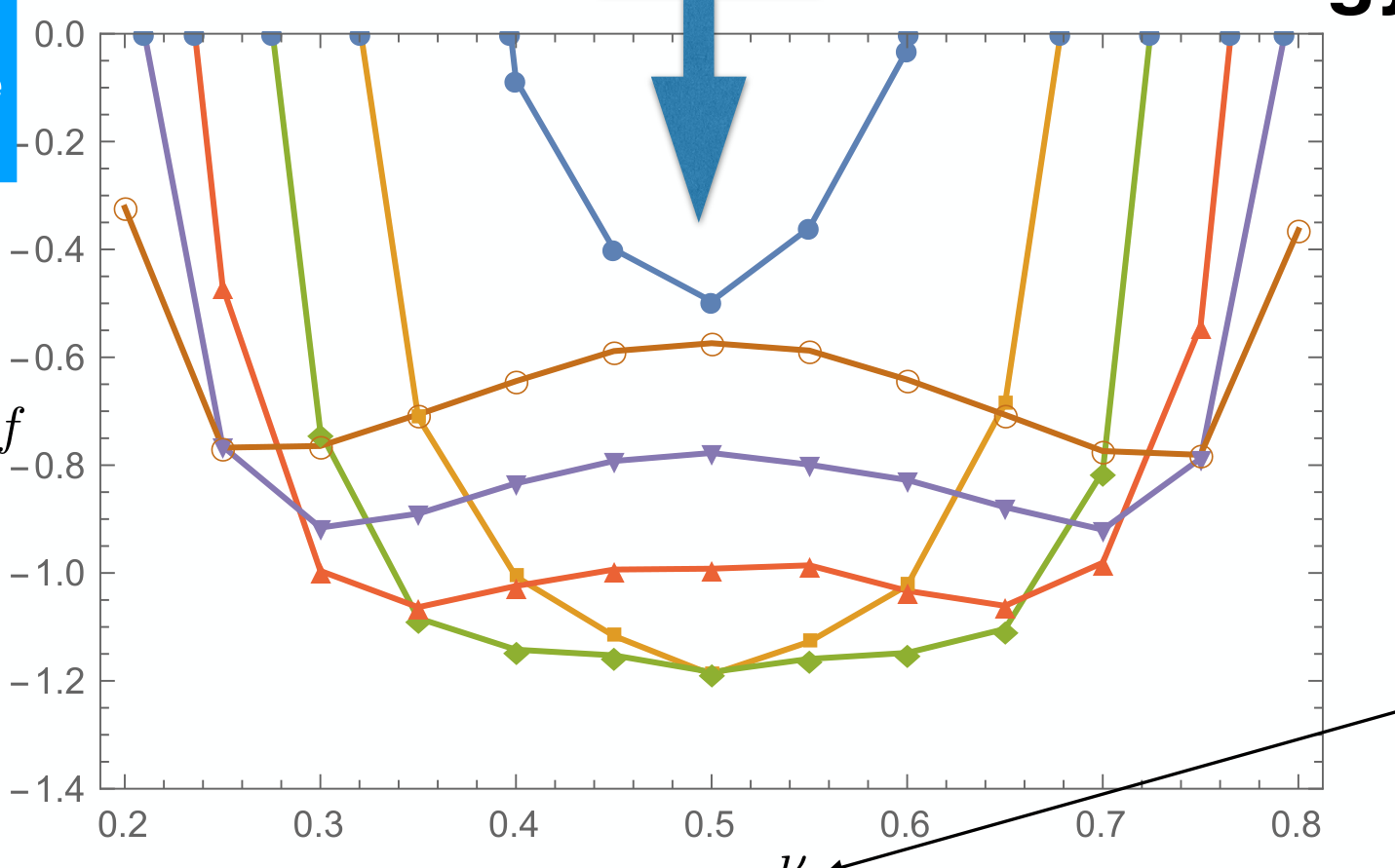
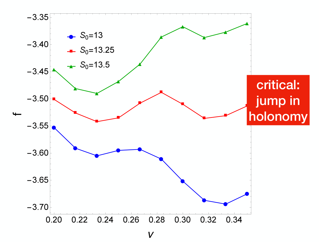
The second nonperturbative issue is chiral symmetry breaking at low . Again, it requires a sufficient density of the dyons, so that their zero modes can get 99 9 Note that already in 1961, the NJL model has shown that one needs a large enough 4-fermion coupling to break chiral symmetry..

9.3 QCD deformation by modified quark periodicity phases
This deformation came first under the name of ”imaginary chemical potentials” [60]. Its usage is different for and deformations. In the former case, the motivation was due to the fact that imaginary chemical potentials can be simulated by usual Monte Carlo algorithms, while those with real cannot. A plot of the lattice results for negative , allows the extrapolation to real , e.g. by Taylor series. This strategy has been used in many lattice studies.
For a large phase, Roberge and Weiss predicted a first order transitions close to , due to different branches of the gluonic GPY potential. Of course, it is a perturbative argument expected to be true at large only. And indeed, when dyons are numerous this transition ends, and according to [61] it happens at .
Another form of deformed QCD is to select imaginary chemical potentials proportional to , so that the quark fugacities are , with certain -independent periodic phases. Moving from conventional (quarks are fermions) to other values, one should see multiple phase transitions, each time when one of the crosses the Polyakov phases , as the fermion zero modes jump from one instanton-dyon to another. The ‘ultimate” selection for theories was proposed in [62], with suggested to be located “democratically”, with one phase located inside each of the holonomy sectors (for ).
In Fig.13 we show ensembles of instanton-dyons simulations for QCD and , with one quark being a fermion and one being a boson. The plots show drastic changes in both phase transitions. Deconfinement changes from a crossover to a strong first order, and chiral restoration is not seen at all 1010 10 Note that SU(2) is somewhat of a special case. If the group is SU(3), and two sectors of dyons would have located in them, ultimately at high these sectors shrink as move towards zero. When they cross phases , the zero modes would return to dyons, and thus at infinite would become similar to undeformed QCD, with chiral symmetry is restored.. We note that the multiply deformed worlds (such as ) are unphysical, and qualitatively different from ours. We expect them to be separated by singularities. Indeed, we recall that has completely different flavor and chiral symmetries (except at high when all are near zero). Its chiral symmetry is split diagonally for all flavors , each broken by diquark ′t Hooft operators for each dyon type. Obviously, this chiral symmetry breaking has no relation to the spontaneously broken chiral symmetry occuring in our world, and due to the multi-quark operators with at finite instanton-dyon density.
Another take on this unusual phases with modified quark periodicities, historically came from supersymmetry. Davies, Hollowood and Khose [63] considered =1 SYM theory on with a small circle and gluinos, and evaluated the quark condensate using instanton-dyons. In this case the gluino term in the GPY potential changes sign, canceling the gluon contribution.
Unsal [64] considered theories with more than one flavor of gluinos (adjoint fermions), . The GPY potential was found to be multiplied by , and for was , favoring confinement at weak coupling (small circle or high ). It was suggested that with confinement present both at small and large , there would be (no phase transitions) at any . However, lattice studies [65] have found deconfined phases in between those two limits, preventing in general such continuity. The considerations based on the GPY potentials at weak coupling (high temperature), do not necessarily carry to strong coupling.
10 Summary
The physics of instantons is now nearly 50 years old, yet we are still finding new applications in the vast land of hadronic physics. Indeed, only recently, the large contributions due to the instanton-antiinstanton molecules came to focus. Recently, we used these contributions to solve two old puzzles. Specifically, the nonperturbative nature of the quark-antiquark potentials, and the large observed mesonic formfactors in the semi-hard regime with few , can be explained by these fields in the QCD vacuum.
The physics of diquarks, first appearing in connection to color superconductivity, again came to the front of spectroscopy, with recent discovery of the double charmed tetraquark state made of .
The development of light front Hamiltonians and wave functions entered a stage at which properties of hadrons, from bottomonium to pions and with all kind of baryons and exotica be systematically calculated. Traditional distinction between heavy and light physics (absence of nonrelativism in the former case) is no longer present on the light front, so all of them are studied in the same setting.
Methods for solving the corresponding equations include variational ones, diagonalization of Hamiltonian written as matrices in appropriate basis, and even direct numerical solutions. This new ”spectroscopy on the light front” program is going to bridge the gap between the usual spectroscopy, the Euclidean version (lattice and instantons) and the light front observables.
The semiclassical theory based on ensembles of instanton-dyons, reproduces semi-quantitatively the main lattice findings about deconfinement in pure gauge theories, and chiral phase transitions, in QCD with light quarks. Deforming QCD by extra action with powers of the Polyakov loop shift/modify the deconfinement transition. Deforming it via quark periodicity phases, leads to phases with drastically different deconfinement and chiral transitions. While all these phases have multiple unphysical properties, their existence shed light on the mechanisms driving the QCD phase transitions. Their key feature are “jumps” of the fermion zero modes, from one dyon type to another.
The dyon zero modes from lattice QCD simulations preserve remarkably well their shapes on the lattice, even in the case of their strong overlaps. Millions of thermal gluons do not seem to affect them.
Finally, we note that instanton-dyon simulations are simple multiple integrals over the instanton-dyon collective variables. So it is relatively easy to get to say of instanton-dyons. In contrast, the lattice simulations which are of course based on first principles, their current cost limit them to about instanton-dyons, as e.g. seen from our Fig.2. If the instanton-dyon ensembles are important for QCD phase transitions as we suggest, then their current values for are perhaps too small to get an accurate description of their phases.
There seems to be enough new land to cover for the next 50 years.
References
- [1] E. Shuryak, Lect. Notes Phys. 977 (2021), 1-520 doi:10.1007/978-3-030-62990-8
- [2] E. V. Shuryak, Nucl. Phys. B 302 (1988), 621-644 doi:10.1016/0550-3213(88)90191-5
- [3] F. Sauter, Z. Phys. 69 (1931), 742-764 doi:10.1007/BF01339461
- [4] A. M. Polyakov, Nucl. Phys. B 120 (1977), 429-458 doi:10.1016/0550-3213(77)90086-4
- [5] A. I. Vainshtein, V. I. Zakharov, V. A. Novikov and M. A. Shifman, Sov. Phys. Usp. 25 (1982), 195 doi:10.1070/PU1982v025n04ABEH004533
- [6] A. A. Aleinikov and E. V. Shuryak, Yad. Fiz. 46 (1987), 122-129
- [7] C. F. Wohler and E. V. Shuryak, Phys. Lett. B 333 (1994), 467-470 doi:10.1016/0370-2693(94)90169-4 [arXiv:hep-ph/9402287 [hep-ph]].
- [8] M. A. Escobar-Ruiz, E. Shuryak and A. V. Turbiner, Phys. Rev. D 92 (2015) no.2, 025046 [erratum: Phys. Rev. D 92 (2015) no.8, 089902] doi:10.1103/PhysRevD.92.025046 [arXiv:1501.03993 [hep-th]].
- [9] A. A. Belavin, A. M. Polyakov, A. S. Schwartz and Y. S. Tyupkin, Phys. Lett. B 59 (1975), 85-87 doi:10.1016/0370-2693(75)90163-X
- [10] G. ’t Hooft, Phys. Rev. D 14 (1976), 3432-3450 [erratum: Phys. Rev. D 18 (1978), 2199] doi:10.1103/PhysRevD.14.3432
- [11] E. Shuryak and J. M. Torres-Rincon, Phys. Rev. C 101 (2020) no.3, 034914 doi:10.1103/PhysRevC.101.034914 [arXiv:1910.08119 [nucl-th]].
- [12] M. A. Escobar-Ruiz, E. Shuryak and A. V. Turbiner, Phys. Rev. D 93 (2016) no.10, 105039 doi:10.1103/PhysRevD.93.105039 [arXiv:1601.03964 [hep-th]].
- [13] Y. Nambu and G. Jona-Lasinio, Phys. Rev. 122 (1961), 345-358 doi:10.1103/PhysRev.122.345
- [14] E. V. Shuryak, Nucl. Phys. B 203 (1982), 140-156 doi:10.1016/0550-3213(82)90480-1
- [15] T. Schäfer and E. V. Shuryak, Rev. Mod. Phys. 70 (1998), 323-426 doi:10.1103/RevModPhys.70.323 [arXiv:hep-ph/9610451 [hep-ph]].
- [16] E. V. Shuryak, Rev. Mod. Phys. 65 (1993), 1-46 doi:10.1103/RevModPhys.65.1
- [17] E. V. Shuryak and J. J. M. Verbaarschot, Phys. Rev. Lett. 68 (1992), 2576-2579 doi:10.1103/PhysRevLett.68.2576
- [18] E. V. Shuryak and J. J. M. Verbaarschot, Nucl. Phys. B 410 (1993), 37-54 doi:10.1016/0550-3213(93)90572-7 [arXiv:hep-ph/9302238 [hep-ph]].
- [19] E. V. Shuryak and J. J. M. Verbaarschot, Nucl. Phys. B 410 (1993), 55-89 doi:10.1016/0550-3213(93)90573-8 [arXiv:hep-ph/9302239 [hep-ph]].
- [20] T. Schäfer, E. V. Shuryak and J. J. M. Verbaarschot, Nucl. Phys. B 412 (1994), 143-168 doi:10.1016/0550-3213(94)90497-9 [arXiv:hep-ph/9306220 [hep-ph]].
- [21] V. Thorsson and I. Zahed, Phys. Rev. D 41, 3442 (1990) doi:10.1103/PhysRevD.41.3442
- [22] T. Schäfer and E. V. Shuryak, Lect. Notes Phys. 578 (2001), 203-217 [arXiv:nucl-th/0010049 [nucl-th]].
- [23] D. M. Ostrovsky, G. W. Carter and E. V. Shuryak, Phys. Rev. D 66 (2002), 036004 doi:10.1103/PhysRevD.66.036004 [arXiv:hep-ph/0204224 [hep-ph]].
- [24] E. Shuryak and I. Zahed, [arXiv:2102.00256 [hep-ph]].
- [25] J. J. M. Verbaarschot, Nucl. Phys. B 362 (1991), 33-53 [erratum: Nucl. Phys. B 386 (1992), 236-236] doi:10.1016/0550-3213(91)90554-B
- [26] V. V. Khoze and A. Ringwald, CERN-TH-6082-91.
- [27] E. Shuryak and I. Zahed, Phys. Rev. D 67 (2003), 014006 doi:10.1103/PhysRevD.67.014006 [arXiv:hep-ph/0206022 [hep-ph]].
- [28] A. Kock, Y. Liu and I. Zahed, Phys. Rev. D 102, no.1, 014039 (2020) doi:10.1103/PhysRevD.102.014039 [arXiv:2004.01595 [hep-ph]].
- [29] A. Kock and I. Zahed, Phys. Rev. D 104, no.11, 116028 (2021) doi:10.1103/PhysRevD.104.116028 [arXiv:2110.06989 [hep-ph]].
- [30] X. Ji, Phys. Rev. Lett. 110, 262002 (2013) doi:10.1103/PhysRevLett.110.262002 [arXiv:1305.1539 [hep-ph]].
- [31] Y. Liu and I. Zahed, [arXiv:2102.07248 [hep-ph]].
- [32] E. Shuryak, Phys. Rev. D 100 (2019) no.11, 114018 doi:10.1103/PhysRevD.100.114018 [arXiv:1908.10270 [hep-ph]].
- [33] A. E. Dorokhov and N. I. Kochelev, Phys. Lett. B 304 (1993), 167-175 doi:10.1016/0370-2693(93)91417-L
- [34] E. Shuryak and I. Zahed, [arXiv:2111.01775 [hep-ph]].
- [35] E. M. Ilgenfritz and E. V. Shuryak, Nucl. Phys. B 319 (1989), 511-520 doi:10.1016/0550-3213(89)90617-2
- [36] R. Rapp, T. Schäfer, E. V. Shuryak and M. Velkovsky, Phys. Rev. Lett. 81 (1998), 53-56 doi:10.1103/PhysRevLett.81.53 [arXiv:hep-ph/9711396 [hep-ph]].
- [37] A. Athenodorou, P. Boucaud, F. De Soto, J. Rodríguez-Quintero and S. Zafeiropoulos, JHEP 02 (2018), 140 doi:10.1007/JHEP02(2018)140 [arXiv:1801.10155 [hep-lat]].
- [38] E. Shuryak and I. Zahed, Phys. Rev. D 103 (2021) no.5, 054028 doi:10.1103/PhysRevD.103.054028 [arXiv:2008.06169 [hep-ph]].
- [39] C. G. Callan, Jr., R. F. Dashen, D. J. Gross, F. Wilczek and A. Zee, Phys. Rev. D 18 (1978), 4684 doi:10.1103/PhysRevD.18.4684
- [40] E. Eichten and F. Feinberg, Phys. Rev. D 23 (1981), 2724 doi:10.1103/PhysRevD.23.2724
- [41] J. F. Arvis, Phys. Lett. B 127 (1983), 106-108 doi:10.1016/0370-2693(83)91640-4
- [42] T. Kawanai and S. Sasaki, Phys. Rev. D 92 (2015) no.9, 094503 doi:10.1103/PhysRevD.92.094503 [arXiv:1508.02178 [hep-lat]].
- [43] E. Meggiolaro, Eur. Phys. J. C 4 (1998), 101-106 doi:10.1007/s100520050189 [arXiv:hep-th/9702186 [hep-th]].
- [44] E. V. Shuryak and I. Zahed, Phys. Rev. D 62 (2000), 085014 doi:10.1103/PhysRevD.62.085014 [arXiv:hep-ph/0005152 [hep-ph]].
- [45] M. Giordano and E. Meggiolaro, eCONF C0906083 (2009), 31 [arXiv:0909.3710 [hep-ph]].
- [46] E. Shuryak and I. Zahed, [arXiv:2111.01775 [hep-ph]].
- [47] M. Musakhanov and U. Yakhshiev, Int. J. Mod. Phys. E 30 (2021) no.11, 2141005 doi:10.1142/S0218301321410056 [arXiv:2103.16628 [hep-ph]].
- [48] K. Langfeld and E. M. Ilgenfritz, Nucl. Phys. B 848 (2011), 33-61 doi:10.1016/j.nuclphysb.2011.02.009 [arXiv:1012.1214 [hep-lat]].
- [49] R. N. Larsen, S. Sharma and E. Shuryak, Phys. Lett. B 794 (2019), 14-18 doi:10.1016/j.physletb.2019.05.019 [arXiv:1811.07914 [hep-lat]].
- [50] R. N. Larsen, S. Sharma and E. Shuryak, Phys. Rev. D 102 (2020) no.3, 034501 doi:10.1103/PhysRevD.102.034501 [arXiv:1912.09141 [hep-lat]].
- [51] E. M. Ilgenfritz and E. V. Shuryak, Phys. Lett. B 325 (1994), 263-266 doi:10.1016/0370-2693(94)90007-8 [arXiv:hep-ph/9401285 [hep-ph]].
- [52] M. Velkovsky and E. V. Shuryak, Phys. Lett. B 437 (1998), 398-402 doi:10.1016/S0370-2693(98)00930-7 [arXiv:hep-ph/9703345 [hep-ph]].
- [53] Y. Liu, E. Shuryak and I. Zahed, Phys. Rev. D 92 (2015) no.8, 085006 doi:10.1103/PhysRevD.92.085006 [arXiv:1503.03058 [hep-ph]].
- [54] Y. Liu, E. Shuryak and I. Zahed, Phys. Rev. D 92 (2015) no.8, 085007 doi:10.1103/PhysRevD.92.085007 [arXiv:1503.09148 [hep-ph]].
- [55] Y. Liu, E. Shuryak and I. Zahed, Phys. Rev. D 98 (2018) no.1, 014023 doi:10.1103/PhysRevD.98.014023 [arXiv:1802.00540 [hep-ph]].
- [56] R. Larsen and E. Shuryak, Phys. Rev. D 92 (2015) no.9, 094022 doi:10.1103/PhysRevD.92.094022 [arXiv:1504.03341 [hep-ph]].
- [57] R. Larsen and E. Shuryak, Phys. Rev. D 93 (2016) no.5, 054029 doi:10.1103/PhysRevD.93.054029 [arXiv:1511.02237 [hep-ph]].
- [58] D. DeMartini and E. Shuryak, Phys. Rev. D 104 (2021) no.5, 054010 doi:10.1103/PhysRevD.104.054010 [arXiv:2102.11321 [hep-ph]].
- [59] D. DeMartini and E. Shuryak, Phys. Rev. D 104 (2021) no.9, 094031 doi:10.1103/PhysRevD.104.094031 [arXiv:2108.06353 [hep-ph]].
- [60] A. Roberge and N. Weiss, Nucl. Phys. B 275 (1986), 734-745 doi:10.1016/0550-3213(86)90582-1
- [61] C. Bonati, M. D’Elia, M. Mariti, M. Mesiti, F. Negro and F. Sanfilippo, Phys. Rev. D 93 (2016) no.7, 074504 doi:10.1103/PhysRevD.93.074504 [arXiv:1602.01426 [hep-lat]].
- [62] H. Kouno, T. Makiyama, T. Sasaki, Y. Sakai and M. Yahiro, J. Phys. G 40 (2013), 095003 doi:10.1088/0954-3899/40/9/095003 [arXiv:1301.4013 [hep-ph]].
- [63] N. M. Davies, T. J. Hollowood, V. V. Khoze and M. P. Mattis, Nucl. Phys. B 559 (1999), 123-142 doi:10.1016/S0550-3213(99)00434-4 [arXiv:hep-th/9905015 [hep-th]].
- [64] M. Unsal, Phys. Rev. D 80 (2009), 065001 doi:10.1103/PhysRevD.80.065001 [arXiv:0709.3269 [hep-th]].
- [65] G. Cossu and M. D’Elia, JHEP 07 (2009), 048 doi:10.1088/1126-6708/2009/07/048 [arXiv:0904.1353 [hep-lat]].
- [66] A. Cherman, T. Schäfer and M. Ünsal, Phys. Rev. Lett. 117 (2016) no.8, 081601 doi:10.1103/PhysRevLett.117.081601 [arXiv:1604.06108 [hep-th]].