Saturated total-population dependent branching process and viral markets Thanks: *The work of first author is partially supported by Prime Minister’s Research Fellowship (PMRF), India.

Social media offers a global platform for communication; people share their content, forward interesting posts among the ones shared with them, etc. It plays a significant role in marketing, e.g., a post advertising a specific product/service can get viral (reach a large number of users). It is also used for spreading propaganda, sharing a piece of knowledge, influencing the beliefs of a large population, etc.

The content propagation (CP) over an online social network (OSN) can be outlined as follows: a) a post is shared with an initial set of users, called seed users; b) the seed users forward the post to their friends/followers if they like it; c) the recipients follow suit and this continues. The content either gets extinct in the initial phase or gets viral, and eventually, copies get saturated, and the propagation ceases.

There are several approaches for studying CP, and we use branching processes (BPs) to analyze the same. Further, since a post can witness a huge surge in the shares in a short duration, we consider continuous-time BPs (e.g., [1, 2, 3]). We discuss and compare other techniques at the end.

Thus the existing BP models are insufficient to mimic a saturated CP due to two imperative factors: a) the overlaps in forwards/offsprings depend upon the total copies/population, and b) the usual content propagation process traverses from super-critical to sub-critical regime before getting extinct. We thus consider a new variant of continuous-time total-population dependent Markovian BP, named as saturated total-population dependent BP (STP-BP). The total copies either increase with time or saturate; if re-forwards are proportional to the total copies, then the resultant value of expected offsprings decreases with time. This also ensures the desired transition from super-critical to sub-critical regime. The saturated BP well mimics the CP.

Recently, we analyzed many new variants of BPs, using a new approach based on stochastic approximation techniques, e.g., attack and acquisition BP (competing viral markets [5]), and proportion-dependent BP (fake news on OSNs [7]). Further modifying the said approach to address the required finite horizon analysis allows us to analyze saturation resulting from total population dependency.

We corroborate our theoretical results by performing Monte-Carlo simulation on SNAP Twitter-dataset [8]. The description of the theoretical trajectories depends only on four parameters of the OSN (e.g., two rates of reduction of the expected forwards) and the attractiveness of the post.

The epidemiology-based models (in particular SIR) are also used to study CP, which succeed in capturing saturation (e.g., [12, 13, 14]). The current and total copies are respectively modelled as infected and (infected$+$recovered) populations. We argue that this approach is not suitable for analyzing viral markets on OSNs/email platforms: (a) this set of literature directly starts with an appropriate ODE (e.g., [13] considers exponentially diminishing infection rate/interest in the post, while [12] considers standard SIR ODE), (b) they do not delve into the details of the random dynamics (e.g., the chance encounters between various individuals), and more importantly, (c) on OSNs, majority of users share the post to a subset of their friends ‘only once’ after viewing and lose interest immediately after; in contrast, in SIR based models, infected individuals keep infecting/spreading the information for a random/prefixed time before recovering/losing-interest. In other words, SIR-based models well capture the typical behaviour of word-of-mouth dynamics (individuals remain interested in gossip, keep sharing it, and then lose interest) and are insufficient for viral markets over OSNs.

There is a brief indirect mention of the saturation effect in [3], where using BPs, the authors predict the future progress of CP using the available history of an ongoing campaign; they use the well-known Kolmogorov’s backward equations (for PGFs in BPs) to achieve this. In contrast, we provide a theoretical study of a new relevant variant of BP, facilitating an exhaustive study of the saturated CP on OSNs.

Consider an OSN where the content of interest is forwarded by its users. At the start of the propagation, the post is shared by its content provider to an initial set of users, called seed users. These users view the post on the OSN at random time instances. Then, they forward it to some or all of their friends, depending on how much they like the post.¹¹ 1 The post may seem appealing to the users for the offers mentioned, the creativity or the informational quotient of the content (see [3]). This subset of users further forward the post when they visit the OSN²² 2 When a user views, reads and forwards some of the posts on its timeline., and the post propagation continues likewise (more details in [1, 5, 3]). The random instances at which users visit the OSN are called wake-up times. The time gap between the wake-up and the post-reception times of any recipient is exponentially distributed with parameter $\lambda$. Let $\mathcal{F}$ be the (random) number of friends of a typical user, with finite mean. The attractiveness of the post is captured by factor $\rho$, which specifies a subset of friends $(\Gamma)$ to whom the post is forwarded. Naturally, $\rho$ determines the growth of the post.

We will see that the content propagation (CP) majorly depends on the expected number of such forwards, which in turn depends on the then total recipients of the post (say $a$). That is, $E[\Gamma]:=m(a)$, where $m$ is some function which will be discussed in detail in the coming sections. The study of such a dependency (using SNAP dataset) and its influence on the CP is the key differentiating feature of our work. As one may anticipate again, such dependency will eventually lead to the reduction in the effective forwards of the post, in turn leading to the saturation of shares. This effect has been observed majorly through numerical studies in the past, e.g., see [1, Fig. 6] and [15, Fig. 1] for total and current shares, respectively. We aim to provide an analytical explanation of saturation in terms of an approximating deterministic trajectory and some relevant performance measures. We next describe the new variant of ‘saturated’ BP, STP-BP.

To facilitate the study of STP-BP, we analyse the embedded chain corresponding to the underlying continuous-time jump process (CTJP), as in [7, 5]. It is a standard technique to use embedded chains, when transience, recurrence, extinction and similar properties of CTJP are studied. We use it for similar purpose in this paper. In particular, we observe the dynamics in (1) at the time instances when a user with unread copy of the post wakes-up. Let $\tau_{n}$ be $n^{th}$ such transition epoch.³³ 3 If the post gets extinct at $n^{th}$ epoch, we set $\tau_{k}:=\tau_{n}$ for all $k\geq n$ and the same is true for rest of the quantities. Let $C_{n}:=C(\tau_{n}^{+})$ be the current shares of the post immediately after $\tau_{n}$. Similarly define $A_{n}$. Note that the time taken by the first user to wake-up after $n^{th}$ transition epoch, ($\tau_{n+1}-\tau_{n}$), is exponentially distributed with parameter $\lambda C_{n}$. Thus, if a user wakes up at $\tau_{n}$, then:

As in [7, 5], we use stochastic approximation (SA) approach to study the embedded chain. Towards this, define the following fractions of current and total shares respectively, $\Psi^{c}_{n}:=\nicefrac{{C_{n}}}{{n}}$ and $\Psi^{a}_{n}:=\nicefrac{{A_{n}}}{{n}}$ for $n\geq 1$, with $\Psi^{c}_{0}=\Psi^{a}_{0}:=a_{0}$. Also let ${\mathbf{\Upsilon}}_{n}:=(\Psi^{c}_{n},\Psi^{a}_{n})$. Further, define:

Then, the evolution of $\Upsilon_{n}$ can be captured by 2-dimensional SA based updates given below (see (2)):

We analyse these fractions using SA techniques (e.g., [16]), which helps in approximating the same using the solutions of the ODE (see (3)):

By Lemma 1, the solution for this non-autonomous and non-smooth ODE exists over any finite time interval in the extended sense (satisfies the ODE for almost all $t$). In Theorem 1 given below, we will prove that the above ODE indeed approximates (2).

Let $\hat{\Upsilon}^{n}(\cdot)$ be the solution of ODE (5), with $\hat{\Upsilon}^{n}(0)=\Upsilon_{n}$. Observe that ${\mathbf{\Upsilon}}^{n}(\cdot)$ in (7) is similar to $\hat{\Upsilon}^{n}(\cdot)$, except for the difference term $\varepsilon^{n}(t):=(\varepsilon^{n,c}(t),\varepsilon^{n,a}(t))$. Further, if at all $\varepsilon^{n}(t)=0$ for all $t\leq T$, then, by uniqueness of the solution (see Lemma 1), the BP trajectory (4) would have coincided with it, i.e., $\Upsilon_{k}=\hat{\Upsilon}(t_{k})$ for all $k$ such that $t_{k}\leq T$. However, it is not true in general; nevertheless, we will show that $||\varepsilon^{n}||\to 0$ as $n\to\infty$ (see norm $||\cdot||$ in (8)).

Thus, we have two operators which are converging towards each other; the first operator including $\varepsilon^{n}$ in (7) provides the BP trajectory, while the second operator without $\varepsilon^{n}$ in (7) provides the ODE solution. Further, using Maximum theorem, we show that the difference between the two solutions of the operators (7) with and without $\varepsilon^{n}$ is small, when $||\varepsilon^{n}||$ is small. Formally, we state the result as follows:

It is clear from the ODE (5) and Theorem 1 that the expected number of forwards, $m(\cdot)$, influence the course of any post; we construct a piece-wise linear function to capture the same. We estimate the parameters and validate the model using the SNAP dataset [8] in section VI. Following aspects are considered for the model:

$\bullet$ Any user on the OSN forwards the post to a subset of friends based on its attractiveness. Among this subset, a fraction of users will have previously received the post. Most likely, such users will not be interested in the same post again. Say $\kappa$ is the fraction of common friends between any two typical users, then $\kappa a$ denotes the number of such re-forwards if ‘$a$’ number of users already had the post. Thus a linearly decreasing function is a suitable choice for $m(\cdot)$.

$\bullet$ It is likely that a user with a high number of friends is also a friend to a large number of users; the dataset supports this observation. Thus, a user with more connections is more likely to receive the post earlier. To capture such aspects, we model the friends of a user, ${\cal F}(a)$, to be independent across users, but with decreasing expected values, i.e., $a\mapsto E[{\cal F}(a)]$ is itself a decreasing function. With this, the assumption (A) is readily satisfied by considering for example, $\hat{\Gamma}={\cal F}(a_{0})$, with $E[{\cal F}(a_{0})]^{2}<\infty$.

$\bullet$ Further, as time progresses, the post would naturally proceed towards saturation. Therefore, it is likely that the slope of $m(\cdot)$ is drastically different towards the end. To summarize, we model the TeF function $m(\cdot)$ as a piece-wise linearly decreasing function, with two different slopes, where the initial slope is bigger than that towards the end.

$\bullet$ It is reasonable to assume that the expected number of forwards is proportional to the attractiveness factor $\rho>0$. Hence, we model the TeF function $m(\cdot)$ as $m(a)=\rho m_{N}(a)\penalty\ \forall\penalty\ a$, where $m_{N}(\cdot)$ is the TeF with $\rho=1$. Such a factorization of $m(\cdot)$ is supported by the experiments on the SNAP dataset for a wide range⁴⁴ 4 Such a common fit is good mostly for $\rho\geq 0.4$, for others we directly derive a good linear fit of $m(\cdot)$ by trial-and-error, see section VI. of $\rho$. The latter function $m_{N}(\cdot)$ is determined solely by the characteristics of the network. Basically, $m_{N}(\cdot)$ corresponds to a hypothetical situation where every recipient shares with all of its friends, but new shares are only the effective forwards. Conclusively:

Thus, the TeF is determined by four parameters, $\bar{m},\kappa_{1},\kappa_{2}$ and ${\bar{a}}$. Here, $\rho\bar{m}=\rho E[\mathcal{F}(a_{0})]$ is the expected number of forwards in the beginning, and $\rho\kappa_{1},\rho\kappa_{2}$ reflect the slopes of the TeF. Observe that the slope reduces to $\rho\kappa_{2}<\rho\kappa_{1}$ when total shares reach a particular value, ${\bar{a}}$. We assume⁵⁵ 5 Then, there is a possibility of exponential growth leading to virality. $\rho\bar{m}>1$.

$\bullet$ We corroborate that the above model well captures the content propagation using an instance of the SNAP dataset: (a) we first obtain the TeF curve by estimating $m_{N}(a)$ (i.e., with $\rho=1$) for some values of $a$; (b) then fit a two slope curve using a naive approach; and (c) use the estimated (four) parameters to derive the solution of the ODE (5) and other theoretical conclusions, for posts with different $\rho$ values.

Estimating the parameters mentioned above in step (b) is crucial in any such study. For now, we estimate the same using a simple trial-and-error method, as explained in footnote 4 and section VI. However, more sophisticated study is essential to estimate these parameters more accurately, and we leave it for the future. As said earlier, this study aims to provide a theoretical understanding of the CP process.

Using the TeF (IV), we solve the ODE (5). By Theorem 1, this solution (a.s.) approximates the CP process. We also derive the approximate trajectories for $a(t)$ and $c(t)$, which show the desirable saturation effect. Let $\tau_{s}:=\inf\{t:a(t)={\bar{a}}\}$ and $\tau_{e}:=\inf\{t:c(t)=0\}$, the extinction time.

In extinction sample paths (we have, $\Upsilon_{n}=0$), from ODE (5), $\hat{\Upsilon}^{n}(t)=0$ $\forall$ $t$. We now consider viral sample paths.

where constants $u:=(u_{1},u_{2},u_{3},u_{4})$ in the two phases equal:

After extinction, i.e, for $t>\tau_{e}$, from the ODE (5), $\psi^{a}(t)=\psi^{a}(\tau_{e})$. Similarly, the current fraction of shares till time $t$ evaluates to the following, again using IF approach:

Further, $\psi^{c}(t)=0$ for all $t\geq\tau_{e}$.

Observe that $a(\cdot)$ saturates as the current shares get extinct. We believe, only STP-BP can capture these effects. Proceeding as in (11), the ODE for $c(t)$ is given by:

By solving, the trajectory of the current shares is given by:

where $\varphi:=\tau_{s}1_{t>\tau_{s}}$. After extinction (for $t\geq\tau_{e}$), $c(t)=0$.

$\displaystyle\hskip-14.22636pta(t_{n})$ $\displaystyle=w_{1}-w_{2}e^{-nw_{3}e^{\gamma}},\mbox{ when }0\leq n\leq n_{e},$ (16) $\displaystyle\hskip-14.22636ptc(t_{n})$ $\displaystyle=w_{1}-w_{2}e^{-nw_{3}e^{\gamma}}-n,\mbox{ when }0\leq n\leq n_{e}.$ (17)

We now investigate other important metrics related to CP.

At this point, we would like to admit that discussing the growth rates at transition epochs is a non-standard practice in the BP literature. However, for the saturated BP, that does not grow forever, we believe such a discussion is relevant and important. In future, we plan to include the influence of $\{\tau_{n}\}$ on these growth rates, by extending the ODE analysis to fractions $\left\{\nicefrac{{\tau_{n}}}{{n}}\right\}$; this would help us derive the standard growth patterns discussed in the BP literature for STP-BP.

where $w$ is given by the second line of (13). Further, by (17), the max reach or saturated total shares $a(t_{n_{e}})$ equal $n_{e}$.

We now perform exhaustive Monte-Carlo (MC) simulations on the SNAP Twitter dataset [8] to validate our theory. The dataset consists of inter-connections among $81,306$ users, with $29.77$ average number of friends. In all the case studies, we consider only viral sample paths.

We repeat the above routine for $\rho=0.4,0.6$ as well, and the corresponding estimates of $m(\cdot)$ are plotted in Fig. 2(i) after dividing by the respective $\rho$ values. The resultant picture gives the confidence that one can derive the individual $m(\cdot)$ curves by using $m_{N}(\cdot)$ as suggested by (IV). We also plot an approximate piece-wise linear curve (see the dashed curve in Fig. 2(i)), with the parameters $\bar{m}=21.321042,\kappa_{1}=532\times 10^{-6},\kappa_{2}=83\times 10^{-6}$ and ${\bar{a}}=35000$ obtained using trial and error method. Henceforth, we refer this $m_{N}(\cdot)$ curve as the common-fit (C-fit) curve. For some sets of simulations, again using the trial and error method, we individually choose best fit $m(\cdot)$ curve for the given case study.

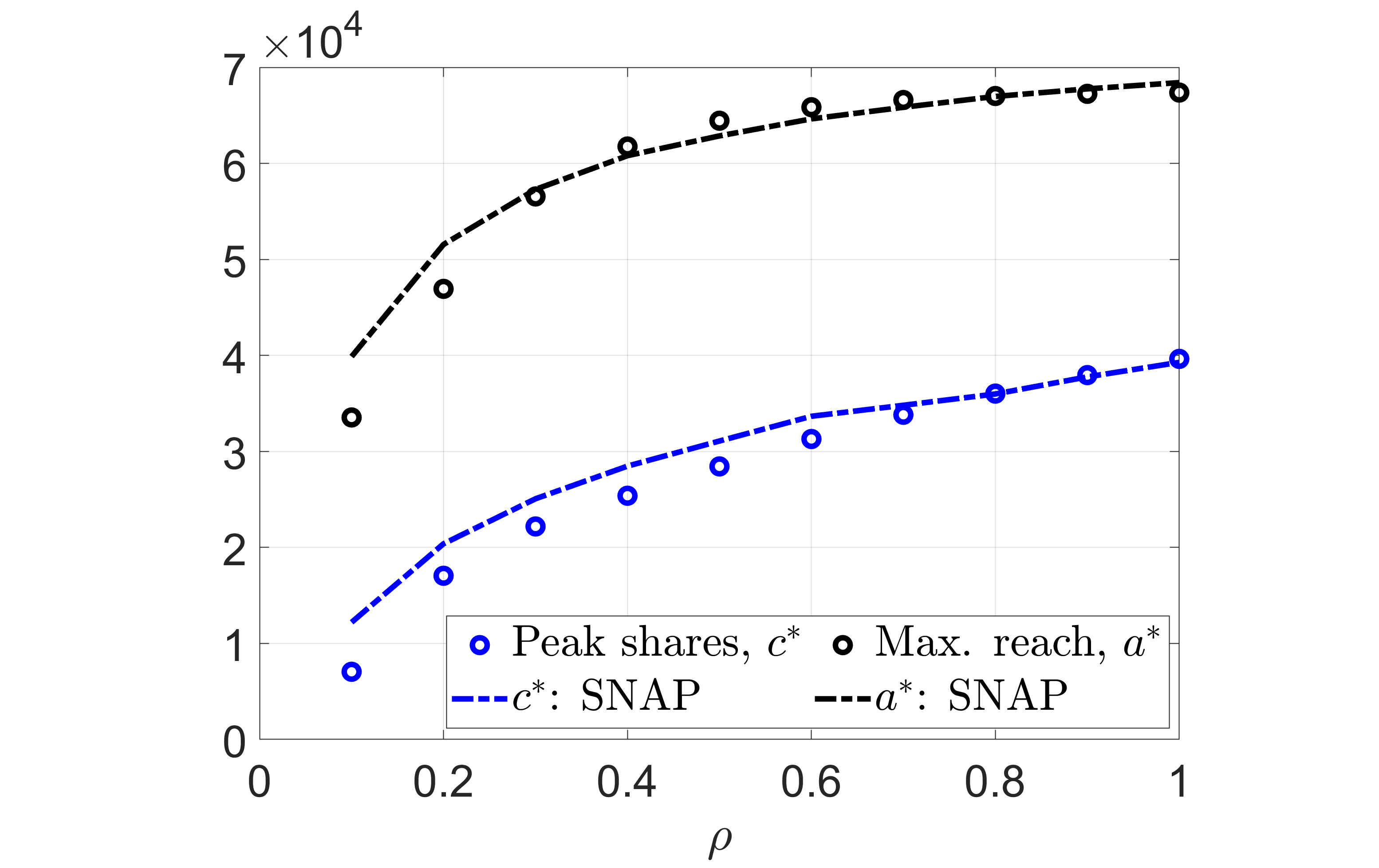
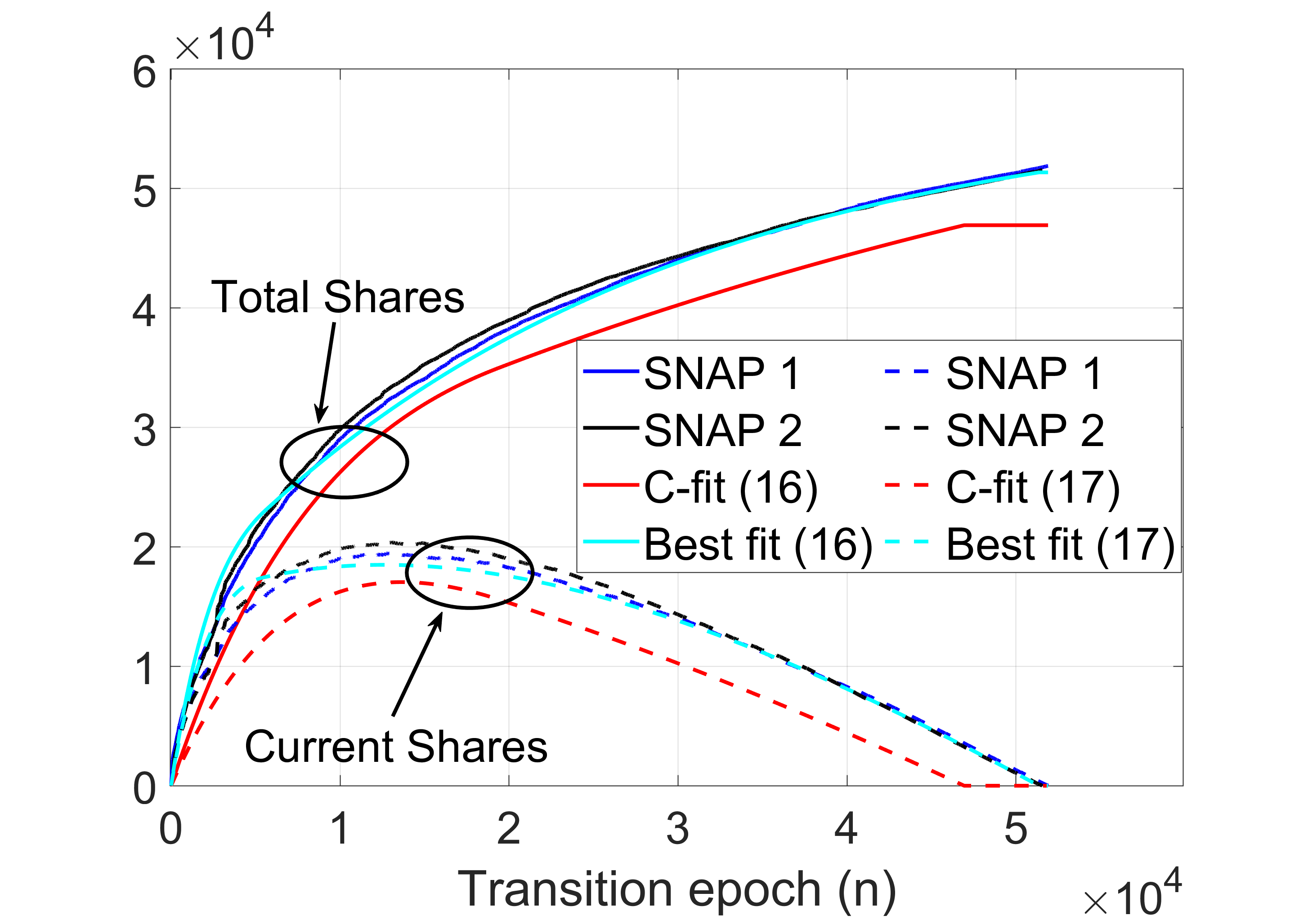
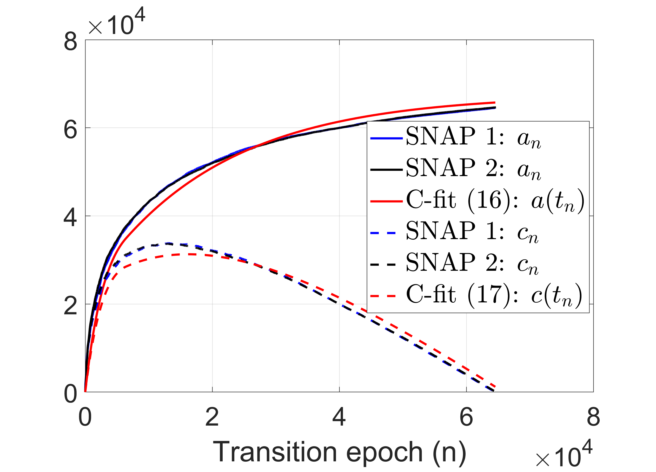
In Fig. 1, we obtain the theoretical curves for total and current shares using C-fit TeF (discussed above), which are then compared with two instances of the CP process on the SNAP dataset. The theoretical curves well approximate the dataset curves for $\rho=0.4,0.6$. In fact, we observed this is true for $\rho\geq 0.4$, in general. However, for lower values of $\rho$ (e.g., $\rho=0.2$ in Fig. 1), the best fit curve better approximates. This suggests that one can obtain C-fit curves for higher and lower ranges of $\rho$ separately. At last in Fig. 2(ii), for different $\rho$ values, we show that the peak shares and max. reach from the C-fit curve approximate the respective values for an instance of CP on the dataset with a maximum error of $11.4645\%$ and $2.4837\%$ respectively (for $\rho\geq 0.4$).

In this paper, we studied the saturation effect experienced by the total shares/copies of the post due to continual re-forwarding on OSNs. We captured the dynamics via newly introduced, saturated total-population dependent branching process. The analysis uses the stochastic approximation technique, which provides an ODE dependent on the post’s total expected (effective) forwards, TeF. We modelled TeF as a piece-wise linearly decreasing function with two slopes. The derived trajectories (dependent on four network-specific parameters) asymptotically and almost surely approximate the total and unread copies over any finite time interval.

Unlike classical dichotomy (either explosion or extinction), the unread copies observe explosion followed by extinction or direct extinction under saturated BPs. Interestingly, maximum reach (number of users that received the post) and the life span (number of users that read the post) are equal. We showed that derived expressions provide a good fit to the simulated instances of propagation over the SNAP dataset. Here, we fitted the parameters of TeF using a naive method; however, advanced methods of estimation/learning can improve the approximation.

Interpolated trajectory. Let ${\mathbf{\Upsilon}}^{n}(\cdot)=(\Psi^{n,c}(\cdot),\Psi^{n,a}(\cdot))$ be the piece-wise interpolated trajectory defined as (see (23)):

Let $\bar{g}({\mathbf{\Upsilon}}_{n},n):=E[L_{n}|\mathcal{F}_{n}]$, i.e., the conditional expectation of $L_{n}$ with respect to ${\cal F}_{n}:=\sigma\{{\mathbf{\Upsilon}}_{k}:1\leq k<n\}$ and $\delta M_{n}:=L_{n}-\bar{g}({\mathbf{\Upsilon}}_{n},n)$. Then, (VIII) can be re-written component-wise as (for each $k\in\{a,c\}$):

It is important to note that $\bar{g}({\mathbf{\Upsilon}}_{n},n)$ is the RHS of the ODE (5) (as $\eta(t_{n})=n$).

Next, we begin by proving that the BP trajectory (see (4)) can be bounded (under assumption (A)) as follows:

By strong law of large numbers, $\hat{\Pi}_{n}\to E[\hat{\Gamma}_{1}]$ a.s. Consider any such sample path ($\omega$). Then, for any $\epsilon>0$, there exists $N_{\epsilon}(\omega)$ such that:

Now, we will prove that $M^{n}(\cdot)=(M^{n,c}(\cdot),M^{n,a}(\cdot))$ and $\rho^{n}(\cdot)$ individually converge to $0$ (as $n\to\infty$) uniformly on any bounded interval. It suffices to prove uniform convergence for sample paths $\omega\in\{\hat{\Pi}_{n}\to b_{1}\}$. We prove the claim for $\psi^{c}$-component, and it can proved analogously for the $\psi^{a}$-component as well. Henceforth, the convergence will be proved w.r.t. $n$, where ever not mentioned explicitly.

Now, define $M_{n}^{c}:=\sum_{i=0}^{n-1}\epsilon_{i}\delta M_{i}^{c}$. Then, it is easy to prove that $(M_{n}^{c})$ is a Martingale with respect to $(\mathcal{F}_{n})$. Thus, using Martingale inequality, for each $\mu>0$ (as in [16, Theorem 2.1, pp. 127]), with $E_{n}(\cdot)$ denoting the expectation conditioned on $(\mathcal{F}_{n})$:

Observe, $E\left[\delta M_{i}^{c}\delta M_{j}^{c}\right]=0$ for $i<j$. Let $O(\omega)$ be the upper-bound on the ODE solution for $t\in[0,T]$, see Lemma 1. Then, from (5) and (VIII),

Thus, under (A), $\sup_{n}E_{n}|L_{n}^{c}-\bar{g}^{c}({\mathbf{\Upsilon}}_{i},t_{i})|^{2}<K$ for some finite $K$. Using this, we have:

By first letting $n\to\infty$ (and using continuity of probability), then, letting $m\to\infty$, for each $\mu>0$, we have:

Now, by (28) and continuity of probability for each $k>0$, $P(A_{k})=1$, where $A_{k}:=\lim_{m\to\infty}\sup_{m\leq j}|M_{j}^{c}-M_{m}^{c}|<1/k$. We further restrict our attention to sample paths $\omega\in N:=(\cap_{k}A_{k})\cap\{\hat{\Pi}_{n}\to b_{1}\}$. For any such $\omega$, using (VIII):

References

- [1] Dhounchak, Ranbir, Veeraruna Kavitha, and Eitan Altman. ”A viral timeline branching process to study a social network.” 2017 29th International Teletraffic Congress (ITC 29). Vol. 3. IEEE, 2017.
- [2] Iribarren, José Luis, and Esteban Moro. ”Branching dynamics of viral information spreading.” Physical Review E 84.4 (2011): 046116.
- [3] Van der Lans, Ralf, et al. ”A viral branching model for predicting the spread of electronic word of mouth.” Marketing science 29.2 (2010): 348-365.
- [4] Athreya, Krishna B., Peter E. Ney, and P. E. Ney. Branching processes. Courier Corporation, 2001.
- [5] Agarwal, Khushboo, and Veeraruna Kavitha. ”Co-Virality of Competing Content over OSNs?.” 2021 IFIP Networking Conference (IFIP Networking). IEEE, 2021.
- [6] Klebaner, Fima Chaim. ”On population-size-dependent branching processes.” Advances in Applied Probability 16.1 (1984): 30-55.
- [7] Kapsikar, Suyog, et al. ”Controlling Fake News by Collective Tagging: A Branching Process Analysis.” IEEE Control Systems Letters 5.6 (2020): 2108-2113.
- [8] Leskovec, Jure, and Julian Mcauley. ”Learning to discover social circles in ego networks.” Advances in neural information processing systems 25 (2012).
- [9] Deijfen, Maria, and Remco van der Hofstad. ”The winner takes it all.” The Annals of Applied Probability 26.4 (2016): 2419-2453.
- [10] Zhou, Jingya, et al. ”Cost-efficient viral marketing in online social networks.” World Wide Web 22.6 (2019): 2355-2378.
- [11] Lu, Xin, et al. ”Beyond the coverage of information spreading: Analytical and empirical evidence of re-exposure in large-scale online social networks.” arXiv preprint arXiv:1907.12389 (2019).
- [12] Rodrigues, Helena Sofia, and Manuel José Fonseca. ”Can information be spread as a virus? Viral marketing as epidemiological model.” Mathematical methods in the applied sciences 39.16 (2016): 4780-4786.
- [13] Freeman, Mark, et al. ”Viral information propagation in the Digg online social network.” Physica A: Statistical Mechanics and its Applications 415 (2014): 87-94.
- [14] Jiang, Ping, and Xiangbin Yan. ”A quantitative model for the spread of online information.” Quality & Quantity 53.4 (2019): 1981-2001.
- [15] Hemsley, Jeff. ”Studying the viral growth of a connective action network using information event signatures.” First monday (2016).
- [16] Harold, J., G. Kushner, and George Yin. ”Stochastic approximation and recursive algorithm and applications.” Springer Science (2003).
- [17] Piccinini, Livio C., Guido Stampacchia, and Giovanni Vidossich. Ordinary differential equations in Rn: problems and methods. Vol. 39. Springer Science & Business Media, 2012.
- [18] Singer, Adam B., and Paul I. Barton. ”Bounding the solutions of parameter dependent nonlinear ordinary differential equations.” SIAM Journal on Scientific Computing 27.6 (2006): 2167-2182.
- [19] Coddington, Earl A., and Norman Levinson. Theory of ordinary differential equations. Tata McGraw-Hill Education, 1955.
- [20] Feinberg, Eugene A., Pavlo O. Kasyanov, and Mark Voorneveld. ”Berge’s maximum theorem for noncompact image sets.” Journal of Mathematical Analysis and Applications 413.2 (2014): 1040-1046.