跳到论文正文
W Papers独立论文阅读器 arXiv:2203.16093 论文正文 计算阅读时间 · 0%
引用这篇论文根据当前论文元数据生成,正式投稿前建议核对。


License: arXiv.org perpetual non-exclusive license
arXiv:2203.16093v2 [cs.IT] 09 Jun 2022

Beamforming Optimization for Active Intelligent Reflecting Surface-Aided SWIPT

Ying Gao    Qingqing Wu    Guangchi Zhang    Wen Chen    Derrick Wing Kwan Ng       Marco Di Renzo Thanks: Y.˜Gao and Q.˜Wu are with the State Key Laboratory of Internet of Things for Smart City, University of Macau, Macao 999078, China (e-mail: yinggao@um.edu.mo; qingqingwu@um.edu.mo). G.˜Zhang is with the School of Information Engineering, Guangdong University of Technology, Guangzhou 510006, China (e-mail: gczhang@gdut.edu.cn). W.˜Chen is with the Department of Electronic Engineering, Shanghai Jiao Tong University, Shanghai 201210, China (e-mail: wenchen@sjtu.edu.cn). D.˜W.˜K.˜Ng is with the School of Electrical Engineering and Telecommunications, University of New South Wales, NSW 2052, Australia (e-mail: w.k.ng@unsw.edu.au). M.˜Di˜Renzo is with Université Paris-Saclay, CNRS, CentraleSupélec, Laboratoire des Signaux et Systèmes, 3 Rue Joliot-Curie, 91192 Gif-sur-Yvette, France. (marco.di-renzo@universite-paris-saclay.fr).
Abstract

Active intelligent reflecting surface (IRS) has been recently proposed to alleviate the product path loss attenuation inherent in the IRS-aided cascaded channel. In this paper, we study an active IRS-aided simultaneous wireless information and power transfer (SWIPT) system. Specifically, an active IRS is deployed to assist a multi-antenna access point (AP) to convey information and energy simultaneously to multiple single-antenna information users (IUs) and energy users (EUs). Two joint transmit and reflect beamforming optimization problems are investigated with different practical objectives. The first problem maximizes the weighted sum-power harvested by the EUs subject to individual signal-to-interference-plus-noise ratio (SINR) constraints at the IUs, while the second problem maximizes the weighted sum-rate of the IUs subject to individual energy harvesting (EH) constraints at the EUs. The optimization problems are non-convex and difficult to solve optimally. To tackle these two problems, we first rigorously prove that dedicated energy beams are not required for their corresponding semidefinite relaxation (SDR) reformulations and the SDR is tight for the first problem, thus greatly simplifying the AP precoding design. Then, by capitalizing on the techniques of alternating optimization (AO), SDR, and successive convex approximation (SCA), computationally efficient algorithms are developed to obtain suboptimal solutions of the resulting optimization problems. Simulation results demonstrate that, given the same total system power budget, significant performance gains in terms of operating range of wireless power transfer (WPT), total harvested energy, as well as achievable rate can be obtained by our proposed designs over benchmark schemes (especially the one adopting a passive IRS). Moreover, it is advisable to deploy an active IRS in the proximity of the users for the effective operation of WPT/SWIPT.

Index Terms: 
Active intelligent reflecting surface (IRS), simultaneous wireless information and power transfer (SWIPT), beamforming optimization, radio frequency-based energy harvesting (EH).

I Introduction

With the increasing number and diversification of intelligent devices in Internet-of-Things (IoT) networks, emerging applications such as smart cities, mobile streaming media, and multisensory virtual reality become possible. One of the main challenges in the roll-out of reliable IoT is the energy limitation of battery-powered devices. Against this background, the dual use of radio frequency (RF) signals for enabling simultaneous wireless information and power transfer (SWIPT) has attracted intense interest [1]. However, energy users (EUs) and information users (IUs) typically operate with very different power sensitivity requirements (e.g., −10-10 dBm for EUs versus −60-60 dBm for IUs) [2]. As such, the operating range of wireless power transfer (WPT) is fundamentally limited by the severe path loss over long signal propagation distances, which restricts the performance of SWIPT systems. Although numerous multiple-input multiple-output (MIMO) technologies can considerably improve the efficiency of both WPT and wireless information transmission (WIT), their practical implementations are still hindered by the required exceedingly high energy consumption and hardware cost [3].

Recently, intelligent reflecting surface (IRS) or reconfigurable intelligent surface (RIS), comprised of a large number of passive metamaterial elements, has emerged as a cost- and energy-efficient solution to unlock the potential of future wireless networks [4, 5, 6, 7, 8]. Specifically, by smartly adapting the phase shifts of all the IRS elements according to the time-varying environment, an IRS is capable of reconfiguring the wireless propagation channels for enhancing the desired signal strength and/or mitigating interference, thus improving the communication performance. It was firstly revealed in [5] that when the number of IRS elements, denoted by NN, is large enough but finite, the receive signal power or the signal-to-noise ratio (SNR) gain scales with 𝒪⁡(N2)\mathcal{O}(N^{2}) asymptotically. This pioneering result has then inspired major interests in studying the joint active and passive beamforming design for various system setups (see, e.g., [9, 10, 11, 12, 13, 14, 15, 16, 17, 18]). While the works [5, 9, 10, 11, 12, 13, 14, 15, 16, 17, 18] mainly focus on exploiting IRSs for effective WIT, the high passive beamforming gain promised by IRSs is also attractive for WPT [1, 4]. To reap this benefit, one line of research investigated IRS-aided wireless-powered communication networks (WPCNs), aiming at improving the communication performance by leveraging an IRS to assist WPT and WIT across different time slots [19, 20, 21, 22]. On the other hand, another line of research focused on exploiting the high passive beamforming gain to enlarge the rate-energy region of SWIPT systems offered by IRSs [23, 24, 25, 26, 27, 28]. For example, the authors of [23] jointly optimized the transmit precoder at the access point (AP) and the phase shifts at the IRS to maximize the weighted sum-power of the EUs, while satisfying the minimum signal-to-interference-plus-noise ratio (SINR) requirements of the IUs. Inspired by [23], the authors of [24] studied the transmit power minimization subject to the individual quality-of-service (QoS) constraints at both the IUs and the EUs. Besides, the weighted sum-rate of all the IUs was maximized in [25], where the weighted sum-power harvested by all the EUs is ensured to be higher than a predefined value for QoS provisioning.

In spite of the appealing advantages of IRSs, the performance of passive IRS-aided systems may not offer a wide coverage extension because of the product path loss attenuation law, unless the number of IRS elements is very large [29]. Particularly, the end-to-end path loss of the transmitter-IRS-receiver link is generally significantly more severe than that of the unobstructed direct link, since the former is the product of the path losses of the transmitter-IRS and the IRS-receiver links. To circumvent this problem, one may need to install a large number of passive reflecting elements and/or to place the passive IRS in close vicinity to either the transmitter or the receiver, which, however, may not always be practically efficient or even feasible. As a remedy, the concept of active IRS has been proposed recently (see, e.g., [30, 31]) to alleviate the product path loss attenuation law. In particular, an active IRS is generally compromised of a number of active reflecting elements, each of which independently integrates a reflection-type amplifier, e.g., a tunnel diode, and thus can not only alter the incident signals’ phases, but also amplify them at the cost of additional low power consumption. Indeed, several papers in the field of metamaterials and communications have proved that an IRS can reflect the incident power with unitary power efficiency, for any angles of incidence and reflection, if local power gains and losses are present along the surface of the IRSs, see, e.g., [32, 33, 34]. The realization of these structures is more difficult than the conventional design of locally-passive IRSs, but it usually results in better performance. The surfaces in [32, 33, 34] are usually globally passive, i.e., the reflected power is not greater than the incident power. In active IRSs, on the other hand, the reflected power is greater than the incident power. Both, however, assume that local power amplifications can be realized along the surface of the IRS. Recently, some innovative efforts have been devoted to beamforming optimization for active IRS-aided systems [30, 31, 35, 36, 37, 38]. For instance, the authors of [30] studied the SNR maximization problem when introducing an active IRS into a single-input multiple-output (SIMO) system. The simulation results demonstrate that, given the same IRS power budget, an active IRS-aided system outperforms its passive counterpart. In [31], it is shown that an active IRS is capable of achieving noticeable capacity gains regardless of the strength of the direct link. Furthermore, the results in [35] indicate that, with the optimized IRS placement, an active IRS has better performance than that of a passive IRS in some practical scenarios.

Although the above works have validated the superiority of adopting an active IRS over a passive IRS under some system setups, to our best knowledge, the potential performance gain of integrating an active IRS into SWIPT systems remains uninvestigated. Moreover, since the information signals for the IUs can be utilized at the EUs for energy harvesting (EH), some fundamental questions remain to be answered in active IRS-aided SWIPT systems. First, are dedicated energy beams required to maximize the weighted sum-power of the EUs with the consideration of information transmission? This question is motivated by the result in [23], which shows that dedicated energy beams are not required for a passive IRS-aided SWIPT system, generalizing the finding in [2] to the case with arbitrary user channels. For active IRS-assisted systems, however, the problem formulation of beamforming design is rather different due to the newly imposed amplification power constraint and the non-negligible IRS-amplified noise power. Thus, it is unknown whether the conclusions drawn in [23] still hold for active IRS-aided SWIPT systems. The second open question is: is sending only information beams sufficient to satisfy the individual EH constraints at the EUs while maximizing the achievable weighted sum-rate of the IUs? In other words, can dedicated energy beams be removed or set to zero when solving the QoS-constrained weighted sum-rate maximization problem? In [25], specially, the authors studied such a problem for a passive IRS-aided SWIPT system, by simply assuming that there is no energy beamforming applied at the AP. Thus, the aforementioned fundamental issues remain unsolved.

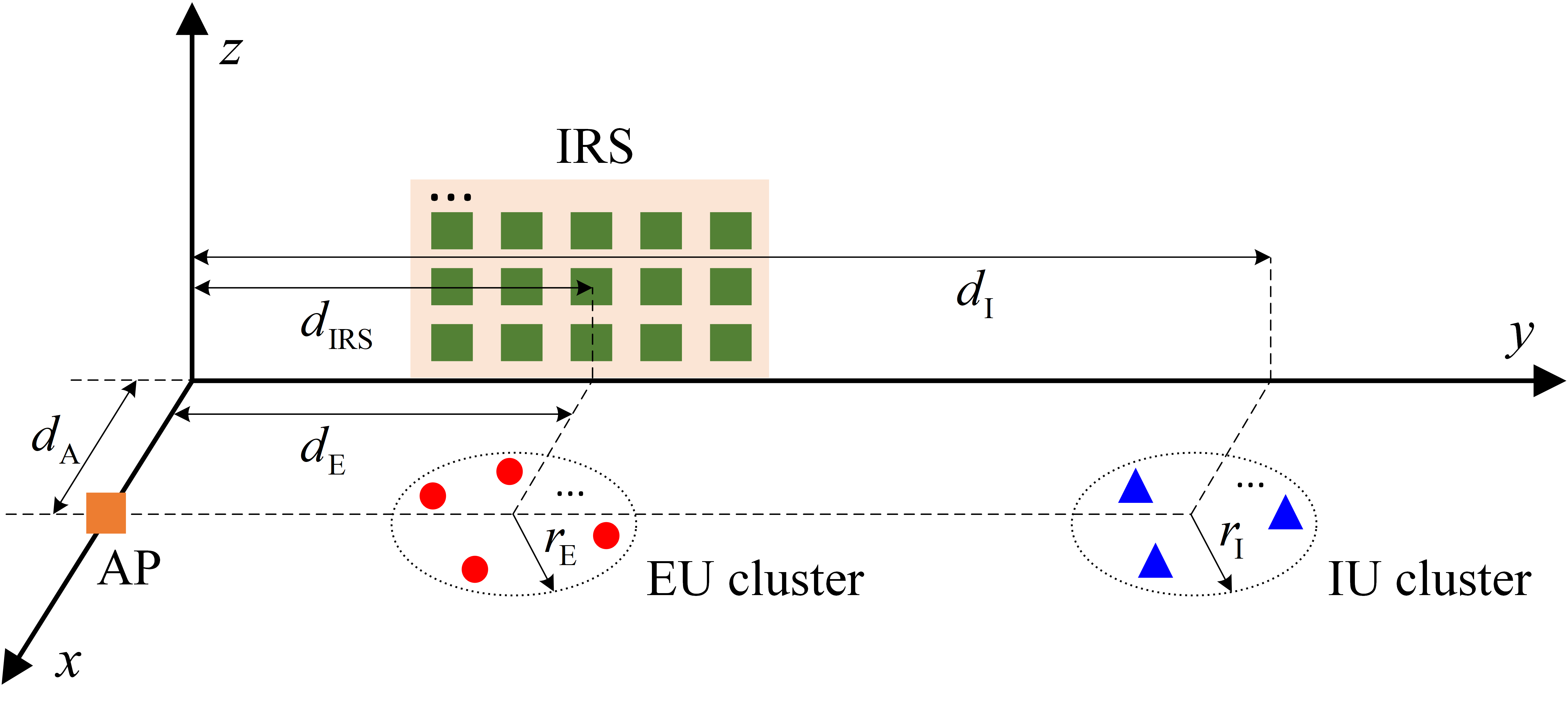
Motivated by these considerations, we investigate an active IRS-aided SWIPT system where an active IRS is deployed to assist the information/power transfer from a multi-antenna AP to multiple single-antenna IUs and EUs, as shown in Fig. 1. The transmit precoder at the AP and the reflection-coefficient matrix at the IRS are jointly optimized by considering two different design criteria. In particular, the first problem maximizes the weighted sum-power harvested by the EUs subject to individual SINR constraints at the IUs, while the second problem maximizes the weighted sum-rate of the IUs subject to individual EH constraints at the EUs. The main contributions of this paper are summarized as follows.

  • •

    To obtain useful insights about active IRS-aided WPT systems, we first consider a special case of the weighted sum-power maximization problem where there exist no IUs and apply the alternating optimization (AO), semidefinite relaxation (SDR), and successive convex approximation (SCA) techniques to obtain a suboptimal solution. Next, for the general case where the EUs and the IUs coexist, we rigorously prove that, despite the presence of a new amplification power constraint and non-negligible IRS-amplified noise power, dedicated energy beams are not required, which greatly simplifies the AP precoding design. Exploiting the obtained insight, we then propose a computationally efficient algorithm to solve the resulting problem suboptimally.

  • •

    For the weighted sum-rate maximization problem, we first unveil that dedicated energy beams are not needed for its SDR reformulation. Additionally, although the tightness of the SDR cannot be confirmed, a high-quality suboptimal solution for the original problem can be constructed from the optimal solution of the reformulated SDR problem. Building upon these insights, we consider the SDR reformulation with no dedicated energy beams to simplify the AP precoding design. Subsequently, we propose a computationally efficient suboptimal algorithm based on the AO and SCA techniques for the resulting problem and show how to approximately recover the transmit precoder if the obtained transmit beamforming matrices are not rank-one.

  • •

    Numerical results demonstrate that by introducing an active IRS, the performance of SWIPT systems can be significantly enhanced in terms of operating range of WPT, total harvested energy, as well as achievable rate, as compared to passive IRS-aided SWIPT systems, under the assumption that the total system power budgets are the same. Furthermore, it is shown that the deployment of an active IRS close to the users is beneficial for WPT/SWIPT systems.

The remainder of this paper is organized as follows. Section II introduces the active IRS-aided SWIPT system model and presents the formulations of the weighted sum-power and sum-rate maximization problems. In Sections III and IV, we propose efficient algorithms for solving the two formulated problems, respectively. Numerical results are presented in Section V to evaluate the performance of the proposed algorithms. Finally, Section VI concludes the paper.

Notations: Scalars, vectors, and matrices are denoted in lower-case, boldface lower-case, and boldface upper-case letters, respectively. ℂx×y\mathbb{C}^{x\times y} denotes the space of x×yx\times y complex-valued matrices. ℍN\mathbb{H}^{N} represents the set of all NN-dimensional complex Hermitian matrices. 𝔼⁡(⋅)\mathbb{E}(\cdot) denotes the statistical expectation. The distribution of a circularly symmetric complex Gaussian (CSCG) random vector with a mean vector 𝒙x and a covariance matrix 𝚺\mathbf{\Sigma} is denoted by 𝒞​𝒩​(𝒙,𝚺)\mathcal{CN}\left(\mbox{\boldmath{$x$}},\mathbf{\Sigma}\right). ∼\sim and ≜\triangleq stand for “distributed as” and “defined as”, respectively. ȷ\jmath denotes the imaginary unit, i.e., ȷ2=1\jmath^{2}=1. The phase and real part of a complex number are denoted by arg⁡(⋅){\rm arg}(\cdot) and Re​{⋅}{\rm Re}\{\cdot\}, respectively. For a vector 𝒂a, ‖𝒂‖\left\|\mbox{\boldmath{$a$}}\right\| and [𝒂]n[\mbox{\boldmath{$a$}}]_{n} represent its Euclidean norm and nn-th element, respectively. diag(𝒂)(\mbox{\boldmath{$a$}}) denotes a diagonal matrix with each diagonal element being the corresponding element in 𝒂a. 𝐈N\mathbf{I}_{N} is an identity matrix of size N×NN\times N; 𝟎\mathbf{0} and 𝟏\mathbf{1} denote an all-zero matrix and an all-one matrix, respectively, with dimensions determined from the context. For a square matrix 𝑺S, tr⁡(𝑺){\rm tr}(\mbox{\boldmath{$S$}}) represents its trace; 𝑺⪰𝟎\mbox{\boldmath{$S$}}\succeq\mbox{\boldmath{$0$}} indicates that 𝑺S is positive semidefinite. For a matrix 𝑨A of arbitrary size, ‖𝑨‖F\left\|\mbox{\boldmath{$A$}}\right\|_{F}, rank⁡(𝑨){\rm rank}(\mbox{\boldmath{$A$}}) and [𝑨]i,j[\mbox{\boldmath{$A$}}]_{i,j} denote its Frobenius norm, rank and (i,j)(i,j)-th element, respectively. (⋅)H(\cdot)^{H} corresponds to the conjugate transport of a vector or matrix. ⊙\odot denotes the Hadamard product. For a set 𝒦\mathcal{K}, |𝒦|\left|\mathcal{K}\right| denotes its cardinality. 𝒪⁡(⋅)\mathcal{O}(\cdot) expresses the big-O notation.

Refer to caption
Fig. 1: An active IRS-aided SWIPT system.

II System Model and Problem Formulation

II-A System Model

As shown in Fig. 1, we consider an active IRS-aided SWIPT system, which comprises an AP with MM antennas, an active IRS11 1 Note that the revealed results and the proposed algorithms in this paper can be extended to the case with a hybrid IRS [39] after slight modifications. with NN reflecting elements, and two sets of single-antenna users, i.e., KIK_{\rm I} IUs and KEK_{\rm E} EUs, denoted by 𝒦ℐ={1,⋯,KI}\mathcal{K_{I}}=\left\{1,\cdots,K_{\rm I}\right\} and 𝒦ℰ={1,⋯,KE}\mathcal{K_{E}}=\left\{1,\cdots,K_{\rm E}\right\}, respectively. In particular, the active IRS is supported by an external power supply and each of its elements can not only alter the incident signals’ phases, but also amplify the incident signals with an integrated reflection-type amplifier. Also, at the AP, we consider a linear transmit precoding for SWIPT with 𝒘i∈ℂM×1\mbox{\boldmath{$w$}}_{i}\in\mathbb{C}^{M\times 1} and 𝒗j∈ℂM×1\mbox{\boldmath{$v$}}_{j}\in\mathbb{C}^{M\times 1} denoting the beamforming vectors for IU ii and EU jj, respectively. Hence, the transmitted signal from the AP can be expressed as

𝒙=∑i∈𝒦ℐ𝒘i​siI+∑j∈𝒦ℰ𝒗j​sjE,\displaystyle\mbox{\boldmath{$x$}}=\sum_{i\in\mathcal{K_{I}}}\mbox{\boldmath{$w$}}_{i}s_{i}^{\rm I}+\sum_{j\in\mathcal{K_{E}}}\mbox{\boldmath{$v$}}_{j}s_{j}^{\rm E}, (1)

where siI∈ℂs_{i}^{\rm I}\in\mathbb{C} and sjE∈ℂs_{j}^{\rm E}\in\mathbb{C} are the information-bearing signal for IU ii and the energy-carrying signal for EU jj, respectively, satisfying siI∼𝒞​𝒩​(0,1)s_{i}^{\rm I}\sim\mathcal{CN}\left(0,1\right), ∀i∈𝒦ℐ\forall i\in\mathcal{K_{I}} and 𝔼⁡(|sjE|2)=1\mathbb{E}\left(\left|s_{j}^{\rm E}\right|^{2}\right)=1, ∀j∈𝒦ℰ\forall j\in\mathcal{K_{E}} [2]. The two signals are assumed to be independent to each other. Let PAP_{\text{A}} denote the total transmit power budget of the AP. From (1), we have 𝔼⁡(𝒙H​𝒙)=∑i∈𝒦ℐ‖𝒘i‖2+∑j∈𝒦ℰ‖𝒗j‖2≤PA\mathbb{E}\left(\mbox{\boldmath{$x$}}^{H}\mbox{\boldmath{$x$}}\right)=\sum_{i\in\mathcal{K_{I}}}\left\|\mbox{\boldmath{$w$}}_{i}\right\|^{2}+\sum_{j\in\mathcal{K_{E}}}\left\|\mbox{\boldmath{$v$}}_{j}\right\|^{2}\leq P_{\text{A}}.

For characterizing the theoretical performance gain brought by an active IRS, we assume a quasi-static fading environment and the channel state information (CSI)22 2 If the IRS is equipped with active sensors, compressive sensing methods [40, 41] can be applied to estimate the channels of the AP-IRS and the IRS-user links, respectively; otherwise, the CSI of individual links can be acquired exploiting some existing methods, e.g., [42, 43]. of all channels involved is assumed to be acquired perfectly by the AP.33 3 It is worth mentioning that although this paper focuses on the case of perfect CSI, the results (i.e., Theorems 1 and 2) can be generalized to the case of imperfect CSI since the proof of Theorems 1 and 2 does not rely on the accuracy of the channel estimation. Note that it is of great interest to develop robust beamforming designs for the case of imperfect CSI, which, however, goes beyond the scope of this paper and is left for future work. Let 𝒉d,iH∈ℂ1×M\mbox{\boldmath{$h$}}_{d,i}^{H}\in\mathbb{C}^{1\times M} and 𝒉r,iH∈ℂ1×N\mbox{\boldmath{$h$}}_{r,i}^{H}\in\mathbb{C}^{1\times N} denote the baseband equivalent channels from the AP to IU ii and from the IRS to IU ii, respectively. The corresponding channels for EU jj are denoted by 𝒈d,jH∈ℂ1×M\mbox{\boldmath{$g$}}_{d,j}^{H}\in\mathbb{C}^{1\times M} and 𝒈r,jH∈ℂ1×N\mbox{\boldmath{$g$}}_{r,j}^{H}\in\mathbb{C}^{1\times N}, respectively, and 𝐅∈ℂN×M\mathbf{F}\in\mathbb{C}^{N\times M} denotes the channel from the AP to the IRS. Let 𝚯=diag​(u1,⋯,uN)∈ℂN×N\mathbf{\Theta}=\text{diag}\left(u_{1},\cdots,u_{N}\right)\in\mathbb{C}^{N\times N} denote the reflection-coefficient matrix at the IRS. Particularly, unu_{n} can be written as un=βn​eȷ​θnu_{n}=\beta_{n}e^{\jmath\theta_{n}}, n∈𝒩≜{1,⋯,N}n\in\mathcal{N}\triangleq\left\{1,\cdots,N\right\}, where βn≥0\beta_{n}\geq 0 and θn∈[0,2​π)\theta_{n}\in[0,2\pi) represent the reflection amplitude and phase shift of the nn-th IRS element, respectively. The signal received at IU ii is then given by

yiI=𝒉d,iH​𝒙⏟direct link+𝒉r,iH​𝚯​(𝐅​𝒙+𝐳)⏟reflected link+ni=(𝒉r,iH​𝚯​𝐅+𝒉d,iH)​𝒙+𝒉r,iH​𝚯​𝐳+ni,i∈𝒦ℐ,\displaystyle y_{i}^{\text{I}}=\underbrace{\mbox{\boldmath{$h$}}_{d,i}^{H}\mbox{\boldmath{$x$}}}_{\text{direct link}}+\underbrace{\mbox{\boldmath{$h$}}_{r,i}^{H}\mbox{\boldmath{$\Theta$}}\left(\mathbf{F}\mbox{\boldmath{$x$}}+\mathbf{z}\right)}_{\text{reflected link}}+n_{i}=\left(\mbox{\boldmath{$h$}}_{r,i}^{H}\mathbf{\Theta}\mathbf{F}+\mbox{\boldmath{$h$}}_{d,i}^{H}\right)\mbox{\boldmath{$x$}}+\mbox{\boldmath{$h$}}_{r,i}^{H}\mathbf{\Theta}\mathbf{z}+n_{i},i\in\mathcal{K_{I}}, (2)

where 𝐳∼𝒞​𝒩​(𝟎,σz2​𝐈N)\mathbf{z}\sim\mathcal{CN}\left(\mathbf{0},\sigma_{z}^{2}\mathbf{I}_{N}\right) and ni∼𝒞​𝒩​(0,σi2)n_{i}\sim\mathcal{CN}\left(0,\sigma_{i}^{2}\right) denote the noise introduced by the active IRS[30] and the additive white Gaussian noise (AWGN) at IU ii, respectively, with σz2\sigma_{z}^{2} and σi2\sigma_{i}^{2} being the corresponding noise variances. By assuming that the interference caused by the energy signals cannot be cancelled by the IUs, the SINR at IU ii can be written as

SINRi=|𝒉iH​𝒘i|2∑k∈𝒦ℐ\{i}|𝒉iH​𝒘k|2+∑j∈𝒦ℰ|𝒉iH​𝒗j|2+σz2​‖𝒉r,iH​𝚯‖2+σi2,i∈𝒦ℐ,\displaystyle\text{SINR}_{i}=\frac{\left|\mbox{\boldmath{$h$}}_{i}^{H}\mbox{\boldmath{$w$}}_{i}\right|^{2}}{\sum_{k\in\mathcal{K_{I}}\backslash\{i\}}\left|\mbox{\boldmath{$h$}}_{i}^{H}\mbox{\boldmath{$w$}}_{k}\right|^{2}+\sum_{j\in\mathcal{K_{E}}}\left|\mbox{\boldmath{$h$}}_{i}^{H}\mbox{\boldmath{$v$}}_{j}\right|^{2}+\sigma_{z}^{2}\left\|\mbox{\boldmath{$h$}}_{r,i}^{H}\mathbf{\Theta}\right\|^{2}+\sigma_{i}^{2}},i\in\mathcal{K_{I}}, (3)

where 𝒉iH≜𝒉r,iH​𝚯​𝐅+𝒉d,iH\mbox{\boldmath{$h$}}_{i}^{H}\triangleq\mbox{\boldmath{$h$}}_{r,i}^{H}\mathbf{\Theta}\mathbf{F}+\mbox{\boldmath{$h$}}_{d,i}^{H} denotes the equivalent end-to-end channel from the AP to IU ii. Accordingly, the achievable rate at IU ii in bits/second/Hz (bps/Hz) is given by Ri=log2⁡(1+SINRi)R_{i}=\log_{2}\left(1+\text{SINR}_{i}\right). On the other hand, the received RF power at EU jj, denoted by QjQ_{j}, can be expressed as

Qj=∑i∈𝒦ℐ|𝒈jH​𝒘i|2+∑m∈𝒦ℰ|𝒈jH​𝒗m|2+σz2​‖𝒈r,jH​𝚯‖2,j∈𝒦ℰ,\displaystyle Q_{j}=\sum_{i\in\mathcal{K_{I}}}\left|\mbox{\boldmath{$g$}}_{j}^{H}\mbox{\boldmath{$w$}}_{i}\right|^{2}+\sum_{m\in\mathcal{K_{E}}}\left|\mbox{\boldmath{$g$}}_{j}^{H}\mbox{\boldmath{$v$}}_{m}\right|^{2}+\sigma_{z}^{2}\left\|\mbox{\boldmath{$g$}}_{r,j}^{H}\mathbf{\Theta}\right\|^{2},j\in\mathcal{K_{E}}, (4)

where 𝒈jH≜𝒈r,jH​𝚯​𝐅+𝒈d,jH\mbox{\boldmath{$g$}}_{j}^{H}\triangleq\mbox{\boldmath{$g$}}_{r,j}^{H}\mathbf{\Theta}\mathbf{F}+\mbox{\boldmath{$g$}}_{d,j}^{H} denotes the equivalent end-to-end channel from the AP to EU jj.44 4 For simplicity, we adopt a linear EH model which is widely used in existing works such as [19, 20, 21, 23, 24, 25]. The extension to the case with a non-linear EH model [27] is discussed in Remarks 3 and 5. Besides, the power of the antenna noise is ignored in EH while that of the noise introduced by the active IRS is considered. This is because the former is generally a negligible constant, while the latter could be non-negligible, especially when the number of the reflecting elements, NN, is sufficiently large.

Suppose that the active IRS is endowed with a maximum amplification power budget PIP_{\text{I}}. Then, we have ∑i∈𝒦ℐ‖𝚯​𝐅​𝒘i‖2+∑j∈𝒦ℰ‖𝚯​𝐅​𝒗j‖2+σz2​‖𝚯‖F2≤PI\sum_{i\in\mathcal{K_{I}}}\left\|\mathbf{\Theta}\mathbf{F}\mbox{\boldmath{$w$}}_{i}\right\|^{2}+\sum_{j\in\mathcal{K_{E}}}\left\|\mathbf{\Theta}\mathbf{F}\mbox{\boldmath{$v$}}_{j}\right\|^{2}+\sigma_{z}^{2}\left\|\mathbf{\Theta}\right\|_{F}^{2}\leq P_{\text{I}}.

II-B Problem Formulation

In this paper, two joint transmit and reflect beamforming optimization problems are considered aiming at two different design criteria. First, we aim to maximize the weighted sum-power received at the EUs while satisfying individual SINR constraints at the IUs, given by γi\gamma_{i}, i∈𝒦ℐi\in\mathcal{K_{I}}. From (4), the weighted sum-power received at the EUs can be written as

∑j∈𝒦ℰαj​Qj=∑i∈𝒦ℐ𝒘iH​𝑺𝒘i+∑j∈𝒦ℰ𝒗jH​𝑺𝒗j+∑j∈𝒦ℰαj​σz2​‖𝒈r,jH​𝚯‖2,\displaystyle\sum_{j\in\mathcal{K_{E}}}\alpha_{j}Q_{j}=\sum_{i\in\mathcal{K_{I}}}\mbox{\boldmath{$w$}}_{i}^{H}\mbox{\boldmath{$S$}}\mbox{\boldmath{$w$}}_{i}+\sum_{j\in\mathcal{K_{E}}}\mbox{\boldmath{$v$}}_{j}^{H}\mbox{\boldmath{$S$}}\mbox{\boldmath{$v$}}_{j}+\sum_{j\in\mathcal{K_{E}}}\alpha_{j}\sigma_{z}^{2}\left\|\mbox{\boldmath{$g$}}_{r,j}^{H}\mathbf{\Theta}\right\|^{2}, (5)

where 𝑺≜∑j∈𝒦ℰαj​𝒈j​𝒈jH\mbox{\boldmath{$S$}}\triangleq\sum_{j\in\mathcal{K_{E}}}\alpha_{j}\mbox{\boldmath{$g$}}_{j}\mbox{\boldmath{$g$}}_{j}^{H} with αj≥0\alpha_{j}\geq 0 denoting the given energy weight for EU jj. Specifically, the larger the value of αj\alpha_{j}, the higher priority to EU jj for EH. Accordingly, the problem of interest can be formulated as

(P1):\displaystyle\hskip-28.45274pt\text{(P1)}: max{𝒘i},{𝒗j},𝚯\displaystyle\underset{\left\{\boldsymbol{w}_{i}\right\},\left\{\boldsymbol{v}_{j}\right\},\mathbf{\Theta}}{\max} ∑i∈𝒦ℐ𝒘iH​𝑺𝒘i+∑j∈𝒦ℰ𝒗jH​𝑺𝒗j+∑j∈𝒦ℰαj​σz2​‖𝒈r,jH​𝚯‖2\displaystyle\sum_{i\in\mathcal{K_{I}}}\mbox{\boldmath{$w$}}_{i}^{H}\mbox{\boldmath{$S$}}\mbox{\boldmath{$w$}}_{i}+\sum_{j\in\mathcal{K_{E}}}\mbox{\boldmath{$v$}}_{j}^{H}\mbox{\boldmath{$S$}}\mbox{\boldmath{$v$}}_{j}+\sum_{j\in\mathcal{K_{E}}}\alpha_{j}\sigma_{z}^{2}\left\|\mbox{\boldmath{$g$}}_{r,j}^{H}\mathbf{\Theta}\right\|^{2} (6a)
s.t. SINRi≥γi,∀i∈𝒦ℐ,\displaystyle\text{SINR}_{i}\geq\gamma_{i},\forall i\in\mathcal{K_{I}}, (6b)
∑i∈𝒦ℐ‖𝒘i‖2+∑j∈𝒦ℰ‖𝒗j‖2≤PA,\displaystyle\sum_{i\in\mathcal{K_{I}}}\left\|\mbox{\boldmath{$w$}}_{i}\right\|^{2}+\sum_{j\in\mathcal{K_{E}}}\left\|\mbox{\boldmath{$v$}}_{j}\right\|^{2}\leq P_{\text{A}}, (6c)
∑i∈𝒦ℐ‖𝚯​𝐅​𝒘i‖2+∑j∈𝒦ℰ‖𝚯​𝐅​𝒗j‖2+σz2​‖𝚯‖F2≤PI.\displaystyle\sum_{i\in\mathcal{K_{I}}}\left\|\mathbf{\Theta}\mathbf{F}\mbox{\boldmath{$w$}}_{i}\right\|^{2}+\sum_{j\in\mathcal{K_{E}}}\left\|\mathbf{\Theta}\mathbf{F}\mbox{\boldmath{$v$}}_{j}\right\|^{2}+\sigma_{z}^{2}\left\|\mathbf{\Theta}\right\|_{F}^{2}\leq P_{\text{I}}. (6d)

Problem (P1) is applicable to the scenarios where the IUs have stringent SINR requirements (e.g., delay-limited transmission) while the EUs only require opportunistic EH.

In addition to (P1), we are also interested in maximizing the weighted sum-rate of the IUs subject to individual EH constraints at the EUs, given by EjE_{j}, j∈𝒦ℰj\in\mathcal{K_{E}}. Let μi\mu_{i} denote the weighting factor that controls the access priority of IU ii. Then, we formulate the optimization problem as follows

(P2):\displaystyle\text{(P2)}: max{𝒘i},{𝒗j},𝚯\displaystyle\underset{\left\{\boldsymbol{w}_{i}\right\},\left\{\boldsymbol{v}_{j}\right\},\mathbf{\Theta}}{\max} ∑i∈𝒦ℐμi​log2⁡(1+SINRi)\displaystyle\sum_{i\in\mathcal{K_{I}}}\mu_{i}\log_{2}\left(1+\text{SINR}_{i}\right) (7a)
s.t. ∑i∈𝒦ℐ|𝒈jH​𝒘i|2+∑m∈𝒦ℰ|𝒈jH​𝒗m|2+σz2​‖𝒈r,jH​𝚯‖2≥Ej,∀j∈𝒦ℰ,\displaystyle\sum_{i\in\mathcal{K_{I}}}\left|\mbox{\boldmath{$g$}}_{j}^{H}\mbox{\boldmath{$w$}}_{i}\right|^{2}+\sum_{m\in\mathcal{K_{E}}}\left|\mbox{\boldmath{$g$}}_{j}^{H}\mbox{\boldmath{$v$}}_{m}\right|^{2}+\sigma_{z}^{2}\left\|\mbox{\boldmath{$g$}}_{r,j}^{H}\mathbf{\Theta}\right\|^{2}\geq E_{j},\forall j\in\mathcal{K_{E}}, (7c)
(6c),(6d).\displaystyle\eqref{cons_PA},\eqref{cons_PI}.

In contrast to (P1), (P2) applies to the scenarios where the EUs impose strict requirements on EH while the IUs have relaxed constraints for information transmission.

Since {𝒘i}\{\mbox{\boldmath{$w$}}_{i}\}, {𝒗j}\{\mbox{\boldmath{$v$}}_{j}\}, and 𝚯\mathbf{\Theta} are intricately coupled in the SINRi\text{SINR}_{i} of IU ii given in (3), the received power QjQ_{j} of EU jj given in (4), and the amplification power constraint given in (6d), optimization problems (P1) and (P2) are both non-convex, and are hence challenging to solve optimally. Moreover, for the considered active IRS-assisted SWIPT system, it remains unknown whether introducing dedicated energy beams {𝒗j}\{\mbox{\boldmath{$v$}}_{j}\} is necessary for achieving the optima of (P1) and (P2) in the presence of information beams {𝒘i}\{\mbox{\boldmath{$w$}}_{i}\}.

III Proposed Solution to Problem (P1)

In this section, we first consider and solve a special case of (P1) with no IUs to gain useful insights into active IRS-aided WPT systems. Then, we answer the question of whether the optimal solution to (P1) requires dedicated energy beams in the general case where the IUs and the EUs coexist. Finally, an efficient algorithm is proposed.

III-A Special Case with No IUs

By setting 𝒘i=𝟎\mbox{\boldmath{$w$}}_{i}=\mathbf{0}, γi=0\gamma_{i}=0, ∀i∈𝒦ℐ\forall i\in\mathcal{K_{I}}, (P1) is simplified to

(P1-NoIUs):\displaystyle\hskip-42.67912pt\text{(P1-NoIUs)}: max{𝒗j},𝚯\displaystyle\underset{\left\{\boldsymbol{v}_{j}\right\},\mathbf{\Theta}}{\max} ∑j∈𝒦ℰ𝒗jH​𝑺𝒗j+∑j∈𝒦ℰαj​σz2​‖𝒈r,jH​𝚯‖2\displaystyle\sum_{j\in\mathcal{K_{E}}}\mbox{\boldmath{$v$}}_{j}^{H}\mbox{\boldmath{$S$}}\mbox{\boldmath{$v$}}_{j}+\sum_{j\in\mathcal{K_{E}}}\alpha_{j}\sigma_{z}^{2}\left\|\mbox{\boldmath{$g$}}_{r,j}^{H}\mathbf{\Theta}\right\|^{2} (8a)
s.t. ∑j∈𝒦ℰ‖𝒗j‖2≤PA,\displaystyle\sum_{j\in\mathcal{K_{E}}}\left\|\mbox{\boldmath{$v$}}_{j}\right\|^{2}\leq P_{\text{A}}, (8b)
∑j∈𝒦ℰ‖𝚯​𝐅​𝒗j‖2+σz2​‖𝚯‖F2≤PI.\displaystyle\sum_{j\in\mathcal{K_{E}}}\left\|\mathbf{\Theta}\mathbf{F}\mbox{\boldmath{$v$}}_{j}\right\|^{2}+\sigma_{z}^{2}\left\|\mathbf{\Theta}\right\|_{F}^{2}\leq P_{\text{I}}. (8c)

The coupling between {𝒗j}\{\mbox{\boldmath{$v$}}_{j}\} and 𝚯\Theta in both the objective function and constraint (8c) introduces non-convexities to (P1-NoIUs). To tackle this issue, we apply the AO method to iteratively optimize {𝒗j}\{\mbox{\boldmath{$v$}}_{j}\} and 𝚯\Theta until convergence is reached, similar to [23] but with the exceptions given below.

III-A1 Optimizing {𝒗j}\{\mbox{\boldmath{$v$}}_{j}\}

For any given 𝚯\mathbf{\Theta}, it was shown in [23] that, without constraint (8c), employing one dedicated energy beam is sufficient to achieve the optimality and the optimal energy precoder should be aligned to the dominant eigenvector of 𝑺S, denoted by 𝒗𝑺v_{S}. However, with the newly introduced constraint (8c), whether employing one dedicated energy beam is sufficient to achieve the optimality is unknown, while aligning the energy precoder to 𝒗𝑺v_{S} may help to improve the objective value to a certain extent but yield a highly suboptimal solution. Therefore, the result in [23] is not directly applicable to the considered problem. In the following, we solve the subproblem with respect to {𝒗j}\{\mbox{\boldmath{$v$}}_{j}\} by applying the SDR technique [44] and answer the aforementioned question. Specifically, we define 𝑾E=∑j∈𝒦ℰ𝒗j​𝒗jH\mbox{\boldmath{$W$}}_{\mathrm{E}}=\sum_{j\in\mathcal{K_{E}}}\mbox{\boldmath{$v$}}_{j}\mbox{\boldmath{$v$}}_{j}^{H}, which needs to satisfy 𝑾E⪰𝟎\mbox{\boldmath{$W$}}_{\mathrm{E}}\succeq\mbox{\boldmath{$0$}} and rank⁡(𝑾E)≤min⁡(M,KE){\rm rank}\left(\mbox{\boldmath{$W$}}_{\mathrm{E}}\right)\leq\min\left(M,K_{\rm E}\right). By relaxing the rank constraint on 𝑾E\mbox{\boldmath{$W$}}_{\mathrm{E}}, the subproblem can be recast as (with some constant terms ignored)

max𝑾E∈ℍM\displaystyle\underset{\boldsymbol{W}_{\mathrm{E}}\in\mathbb{H}^{M}}{\max} tr​(𝑺𝑾E)\displaystyle\text{tr}\left(\mbox{\boldmath{$S$}}\mbox{\boldmath{$W$}}_{\mathrm{E}}\right) (9a)
s.t. tr⁡(𝑾E)≤PA,tr⁡(𝑪𝑾E)≤P¯I,𝑾E⪰𝟎,\displaystyle{\rm tr}\left(\mbox{\boldmath{$W$}}_{\mathrm{E}}\right)\leq P_{\text{A}},\ {\rm tr}\left(\mbox{\boldmath{$C$}}\mbox{\boldmath{$W$}}_{\mathrm{E}}\right)\leq\bar{P}_{\text{I}},\ \mbox{\boldmath{$W$}}_{\mathrm{E}}\succeq\mbox{\boldmath{$0$}}, (9b)

where 𝑪≜𝐅H​𝚯H​𝚯​𝐅\mbox{\boldmath{$C$}}\triangleq\mathbf{F}^{H}\mbox{\boldmath{$\Theta$}}^{H}\mbox{\boldmath{$\Theta$}}\mathbf{F} and P¯I≜PI−σz2​‖𝚯‖F2\bar{P}_{\text{I}}\triangleq P_{\text{I}}-\sigma_{z}^{2}\left\|\mathbf{\Theta}\right\|_{F}^{2}. As problem (9) is a convex semidefinite program (SDP), it can be optimally solved by existing convex optimization solvers, e.g., CVX [45]. Regarding the rank of the obtained optimal solution, we have the following remark.

Remark 1.

According to [46, Theorem 3.2], there exists an optimal solution 𝑾E∗\mbox{\boldmath{$W$}}_{\mathrm{E}}^{*} to problem (9) such that (rank⁡(𝑾E∗))2≤2\left({\rm rank}\left(\mbox{\boldmath{$W$}}_{\mathrm{E}}^{*}\right)\right)^{2}\leq 2, where 22 corresponds to the number of linear constraints in (9). Moreover, if PA>0P_{\rm A}>0 and P¯I>0\bar{P}_{\rm I}>0, 𝑾E∗=𝟎\mbox{\boldmath{$W$}}_{\mathrm{E}}^{*}=\mathbf{0} cannot be the optimal solution. Hence, an optimal solution that fulfills rank⁡(𝑾E∗)=1{\rm rank}\left(\mbox{\boldmath{$W$}}_{\mathrm{E}}^{*}\right)=1 should exist for problem (9).

Although Remark 1 only indicates the existence of a rank-one optimal solution, the rank-reduction techniques in [46] can always be applied to construct a rank-one optimal solution from its non-rank-one optimal counterpart. Once obtained, 𝑾E∗\mbox{\boldmath{$W$}}_{\mathrm{E}}^{*} can be decomposed as 𝑾E∗=𝒗0∗​(𝒗0∗)H\mbox{\boldmath{$W$}}_{\mathrm{E}}^{*}=\mbox{\boldmath{$v$}}_{0}^{*}\left(\mbox{\boldmath{$v$}}_{0}^{*}\right)^{H} via the Cholesky decomposition to recover the desired energy beamforming vector. Thus, we can choose to send only one energy beam to simplify the transmitter implementation by setting 𝒗k=𝒗0∗\mbox{\boldmath{$v$}}_{k}=\mbox{\boldmath{$v$}}_{0}^{*} for any k∈𝒦ℰk\in\mathcal{K_{E}} and 𝒗j=𝟎\mbox{\boldmath{$v$}}_{j}=\mathbf{0}, ∀j∈𝒦ℰ\{k}\forall j\in\mathcal{K_{E}}\backslash\{k\}.

III-A2 Optimizing 𝚯\mathbf{\Theta}

For any given 𝒗0∗\mbox{\boldmath{$v$}}_{0}^{*}, 𝚯\mathbf{\Theta} can be optimized by solving (P1-NoIUs) with only the constraint in (8c). To facilitate the solution design, we define 𝒖=[u1,⋯,uN]H\mbox{\boldmath{$u$}}=\left[u_{1},\cdots,u_{N}\right]^{H}, 𝒖¯=[𝒖;1]\bar{\mbox{\boldmath{$u$}}}=\left[\mbox{\boldmath{$u$}};1\right], 𝐆j=[diag​(𝒈r,jH)​𝐅;𝒈d,jH]\mathbf{G}_{j}=\left[\text{diag}\left(\mbox{\boldmath{$g$}}_{r,j}^{H}\right)\mathbf{F};\mbox{\boldmath{$g$}}_{d,j}^{H}\right], 𝐙j=diag​([𝒈r,jH,0])​diag​([𝒈r,j;0])\mathbf{Z}_{j}=\text{diag}\left(\left[\mbox{\boldmath{$g$}}_{r,j}^{H},0\right]\right)\text{diag}\left(\left[\mbox{\boldmath{$g$}}_{r,j};0\right]\right), 𝚽=diag​([𝐅​𝒗0∗;0])​(diag​([𝐅​𝒗0∗;0]))H\mathbf{\Phi}=\text{diag}\left(\left[\mathbf{F}\mbox{\boldmath{$v$}}_{0}^{*};0\right]\right)\left(\text{diag}\left(\left[\mathbf{F}\mbox{\boldmath{$v$}}_{0}^{*};0\right]\right)\right)^{H}, and 𝐏=diag​([𝟏N×1;0])\mathbf{P}=\text{diag}\left(\left[\mathbf{1}_{N\times 1};0\right]\right). Then, we have 𝒈r,jH​𝚯​𝐅+𝒈d,jH=𝒖¯H​𝐆j\mbox{\boldmath{$g$}}_{r,j}^{H}\mathbf{\Theta}\mathbf{F}+\mbox{\boldmath{$g$}}_{d,j}^{H}=\bar{\mbox{\boldmath{$u$}}}^{H}\mathbf{G}_{j}, ‖𝒈r,jH​𝚯‖2=𝒖¯H​𝐙j​𝒖¯\left\|\mbox{\boldmath{$g$}}_{r,j}^{H}\mathbf{\Theta}\right\|^{2}=\bar{\mbox{\boldmath{$u$}}}^{H}\mathbf{Z}_{j}\bar{\mbox{\boldmath{$u$}}}, ‖𝚯​𝐅​𝒗0∗‖2=𝒖¯H​𝚽​𝒖¯\left\|\mathbf{\Theta}\mathbf{F}\mbox{\boldmath{$v$}}_{0}^{*}\right\|^{2}=\bar{\mbox{\boldmath{$u$}}}^{H}\mathbf{\Phi}\bar{\mbox{\boldmath{$u$}}}, and ‖𝚯‖F2=𝒖¯H​𝐏​𝒖¯\left\|\mathbf{\Theta}\right\|_{F}^{2}=\bar{\mbox{\boldmath{$u$}}}^{H}\mathbf{P}\bar{\mbox{\boldmath{$u$}}}. As a result, the subproblem is equivalent to

max𝒖¯\displaystyle\underset{\bar{\boldsymbol{u}}}{\max} ∑j∈𝒦ℰαj​|𝒖¯H​𝐆j​𝒗0∗|2+∑j∈𝒦ℰαj​σz2​𝒖¯H​𝐙j​𝒖¯\displaystyle\sum_{j\in\mathcal{K_{E}}}\alpha_{j}\left|\bar{\mbox{\boldmath{$u$}}}^{H}\mathbf{G}_{j}\mbox{\boldmath{$v$}}_{0}^{*}\right|^{2}+\sum_{j\in\mathcal{K_{E}}}\alpha_{j}\sigma_{z}^{2}\bar{\mbox{\boldmath{$u$}}}^{H}\mathbf{Z}_{j}\bar{\mbox{\boldmath{$u$}}} (10a)
s.t. 𝒖¯H​𝚽​𝒖¯+σz2​𝒖¯H​𝐏​𝒖¯≤PI,\displaystyle\bar{\mbox{\boldmath{$u$}}}^{H}\mathbf{\Phi}\bar{\mbox{\boldmath{$u$}}}+\sigma_{z}^{2}\bar{\mbox{\boldmath{$u$}}}^{H}\mathbf{P}\bar{\mbox{\boldmath{$u$}}}\leq P_{\text{I}}, (10b)
[𝒖¯]N+1=1.\displaystyle[\bar{\mbox{\boldmath{$u$}}}]_{N+1}=1. (10c)

Although maximizing a convex function results in a non-convex problem [45], the convexity of the objective function in (10a) allows us to apply the iterative SCA technique for solving problem (10) suboptimally. To begin with, the objective function can be written in a compact form as 𝒖¯H​𝐀​𝒖¯\bar{\mbox{\boldmath{$u$}}}^{H}\mathbf{A}\bar{\mbox{\boldmath{$u$}}}, where 𝐀=∑j∈𝒦ℰαj​(𝐆j​𝒗0∗​(𝒗0∗)H​𝐆jH+σz2​𝐙j)≥0\mathbf{A}=\sum_{j\in\mathcal{K_{E}}}\alpha_{j}\left(\mathbf{G}_{j}\mbox{\boldmath{$v$}}_{0}^{*}(\mbox{\boldmath{$v$}}_{0}^{*})^{H}\mathbf{G}_{j}^{H}+\sigma_{z}^{2}\mathbf{Z}_{j}\right)\geq 0. Next, for a given local feasible point 𝒖¯(l)\bar{\mbox{\boldmath{$u$}}}^{(l)} in the ll-th iteration, the first-order Taylor expansion is a lower bound for 𝒖¯H​𝐀​𝒖¯\bar{\mbox{\boldmath{$u$}}}^{H}\mathbf{A}\bar{\mbox{\boldmath{$u$}}} that can be expressed as

𝒖¯H​𝐀​𝒖¯≥2​R​e​{𝒖¯H​𝐀​𝒖¯(l)}−(𝒖¯(l))H​𝐀​𝒖¯(l)≜𝒢(l)​(𝒖¯).\displaystyle\bar{\mbox{\boldmath{$u$}}}^{H}\mathbf{A}\bar{\mbox{\boldmath{$u$}}}\geq 2{\rm Re}\left\{{\bar{\mbox{\boldmath{$u$}}}^{H}\mathbf{A}\bar{\mbox{\boldmath{$u$}}}^{(l)}}\right\}-\left(\bar{\mbox{\boldmath{$u$}}}^{(l)}\right)^{H}\mathbf{A}\bar{\mbox{\boldmath{$u$}}}^{(l)}\triangleq\mathcal{G}^{(l)}(\bar{\mbox{\boldmath{$u$}}}). (11)

By replacing the objective function in (10a) with 𝒢(l)​(𝒖¯)\mathcal{G}^{(l)}(\bar{\mbox{\boldmath{$u$}}}), a suboptimal solution to (10) can be obtained by solving the following convex quadratically constrained quadratic program (QCQP):

max𝒖¯​𝒢(l)​(𝒖¯)s.t.​(10b),(10c).\displaystyle\underset{\bar{\boldsymbol{u}}}{\max}\ \mathcal{G}^{(l)}(\bar{\mbox{\boldmath{$u$}}})\hskip 11.38109pt\text{s.t.}\ \eqref{WPT_sub2_equiv_cons1},\eqref{WPT_sub2_equiv_cons2}. (12)
Remark 2.

It is observed that the value of the LHS of constraint (10b) is independent of the phase value of each element in 𝒖¯\bar{\mbox{\boldmath{$u$}}}. Therefore, the optimal phase of unu_{n} can be obtained in a closed-form expression given by θn∗=0\theta_{n}^{*}=0 if [𝐀​𝒖¯(l)]n=0\left[\mathbf{A}\bar{\mbox{\boldmath{$u$}}}^{(l)}\right]_{n}=0 and θn∗=arg⁡([𝐀​𝒖¯(l)]n)\theta_{n}^{*}={\rm arg}\left(\left[\mathbf{A}\bar{\mbox{\boldmath{$u$}}}^{(l)}\right]_{n}\right) otherwise, ∀n\forall n. Subsequently, only the real-number magnitudes of {un}\{u_{n}\} are needed to be optimized by solving problem (12) via existing convex optimization solvers, e.g., CVX [45]. This helps to reduce the simulation time.

III-A3 Convergence and Complexity Analysis

As the objective value of (P1-NoIUs) is non-decreasing over the iterations and also upper-bounded by a finite value, the proposed algorithm is guaranteed to converge. Besides, the main computational burden stems from solving the SDP in (9) and the QCQP in (12). Simply speaking, given a solution accuracy ε\varepsilon, problem (9) can be solved with a computational complexity55 5 According to [47], for an SDP problem with mm SDP constraints, each of which involves an nn-dimensional positive semidefinite matrix, the computational complexity for solving it is given by 𝒪⁡(n​log⁡(1ε)​(m​n3+m2​n2+m3))\mathcal{O}\left(\sqrt{n}\log\left(\frac{1}{\varepsilon}\right)\left(mn^{3}+m^{2}n^{2}+m^{3}\right)\right). For the SDP in (9), we have m=2m=2 and n=Mn=M. of 𝒪⁡(M3.5​log⁡(1ε))\mathcal{O}\left(M^{3.5}\log(\frac{1}{\varepsilon})\right), while the arithmetic cost66 6 According to [48], the arithmetic cost for solving a QCQP problem with mm variables and nn quadratic constraints is given by 𝒪⁡(m​(m​n2+n3)​ln⁡(2​m​Vε))\mathcal{O}\left(\sqrt{m}\left(mn^{2}+n^{3}\right)\ln\left(\frac{2mV}{\varepsilon}\right)\right). For the QCQP in (12), we have m=N+1m=N+1 and n=2n=2. of solving problem (12) is less than 𝒪⁡(N1.5​ln⁡(2​(N+1)​Vε))\mathcal{O}\left(N^{1.5}\ln\left(\frac{2(N+1)V}{\varepsilon}\right)\right), where VV is a constant defined in [48] and V>εV>\varepsilon. Thus, the total complexity of the proposed algorithm is about

𝒪⁡[Υ⁡(M3.5​log⁡(1ε)+N1.5​ln⁡(2​(N+1)​Vε))],\displaystyle\mathcal{O}\left[\Upsilon\left(M^{3.5}\log\left(\frac{1}{\varepsilon}\right)+N^{1.5}\ln\left(\frac{2(N+1)V}{\varepsilon}\right)\right)\right], (13)

with Υ\Upsilon denoting the number of iterations required for convergence.

III-B Are Dedicated Energy Beams Necessary?

Here, the general case where at least one IU coexists with KEK_{\rm E} EUs is studied. In addition to the variables 𝑪C, P¯I\bar{P}_{\text{I}}, and 𝑾E\mbox{\boldmath{$W$}}_{\mathrm{E}} defined in the previous subsection, we define 𝑾i=𝒘i​𝒘iH\mbox{\boldmath{$W$}}_{i}=\mbox{\boldmath{$w$}}_{i}\mbox{\boldmath{$w$}}_{i}^{H}, ∀i∈𝒦ℐ\forall i\in\mathcal{K_{I}}. Then, it follows that 𝑾i⪰𝟎\mbox{\boldmath{$W$}}_{i}\succeq\mbox{\boldmath{$0$}} and rank⁡(𝑾i)≤1{\rm rank}\left(\mbox{\boldmath{$W$}}_{i}\right)\leq 1, ∀i∈𝒦ℐ\forall i\in\mathcal{K_{I}}. By dropping the rank constraints on 𝑾E\mbox{\boldmath{$W$}}_{\mathrm{E}} and {𝑾i}\{\mbox{\boldmath{$W$}}_{i}\}, the SDR reformulation of (P1) can be expressed as

(P1-SDR1):\displaystyle\hskip-42.67912pt\text{(P1-SDR1)}: max{𝑾i∈ℍM},𝑾E∈ℍM,𝚯\displaystyle\underset{\begin{subarray}{c}\left\{\boldsymbol{W}_{i}\in\mathbb{H}^{M}\right\},\\ \boldsymbol{W}_{\mathrm{E}}\in\mathbb{H}^{M},\mathbf{\Theta}\end{subarray}}{\max} ∑i∈𝒦ℐtr⁡(𝑺𝑾i)+tr⁡(𝑺𝑾E)+∑j∈𝒦ℰαj​σz2​‖𝒈r,jH​𝚯‖2\displaystyle\sum_{i\in\mathcal{K_{I}}}{\rm tr}\left(\mbox{\boldmath{$S$}}\mbox{\boldmath{$W$}}_{i}\right)+{\rm tr}\left(\mbox{\boldmath{$S$}}\mbox{\boldmath{$W$}}_{\mathrm{E}}\right)+\sum_{j\in\mathcal{K_{E}}}\alpha_{j}\sigma_{z}^{2}\left\|\mbox{\boldmath{$g$}}_{r,j}^{H}\mathbf{\Theta}\right\|^{2} (14a)
s.t. tr⁡(𝒉i​𝒉iH​𝑾i)γi−∑k∈𝒦ℐ\{i}tr⁡(𝒉i​𝒉iH​𝑾k)−tr⁡(𝒉i​𝒉iH​𝑾E)\displaystyle\frac{{\rm tr}\left(\mbox{\boldmath{$h$}}_{i}\mbox{\boldmath{$h$}}_{i}^{H}\mbox{\boldmath{$W$}}_{i}\right)}{\gamma_{i}}-\sum_{k\in\mathcal{K_{I}}\backslash\{i\}}{\rm tr}\left(\mbox{\boldmath{$h$}}_{i}\mbox{\boldmath{$h$}}_{i}^{H}\mbox{\boldmath{$W$}}_{k}\right)-{\rm tr}\left(\mbox{\boldmath{$h$}}_{i}\mbox{\boldmath{$h$}}_{i}^{H}\mbox{\boldmath{$W$}}_{\mathrm{E}}\right)
−σ¯i2≥0,∀i∈𝒦ℐ,\displaystyle-\bar{\sigma}_{i}^{2}\geq 0,\forall i\in\mathcal{K_{I}}, (14c)
∑i∈𝒦ℐtr⁡(𝑾i)+tr⁡(𝑾E)≤PA,\displaystyle\sum_{i\in\mathcal{K_{I}}}{\rm tr}\left(\mbox{\boldmath{$W$}}_{i}\right)+{\rm tr}\left(\mbox{\boldmath{$W$}}_{\mathrm{E}}\right)\leq P_{\text{A}},
∑i∈𝒦ℐtr⁡(𝑪𝑾i)+tr⁡(𝑪𝑾E)≤P¯I,\displaystyle\sum_{i\in\mathcal{K_{I}}}{\rm tr}\left(\mbox{\boldmath{$C$}}\mbox{\boldmath{$W$}}_{i}\right)+{\rm tr}\left(\mbox{\boldmath{$C$}}\mbox{\boldmath{$W$}}_{\mathrm{E}}\right)\leq\bar{P}_{\text{I}}, (14e)
𝑾i⪰𝟎,∀i∈𝒦ℐ,𝑾E⪰𝟎,\displaystyle\mbox{\boldmath{$W$}}_{i}\succeq\mathbf{0},\forall i\in\mathcal{K_{I}},\;\mbox{\boldmath{$W$}}_{\mathrm{E}}\succeq\mathbf{0},

where σ¯i2≜σz2​‖𝐡r,iH​𝚯‖2+σi2\bar{\sigma}_{i}^{2}\triangleq\sigma_{z}^{2}\left\|\mathbf{h}_{r,i}^{H}\mathbf{\Theta}\right\|^{2}+\sigma_{i}^{2}, ∀i∈𝒦ℐ\forall i\in\mathcal{K_{I}}. If we remove constraint (14e), neglect the IRS-amplified noise power in (14a) and (14c), and set βn=1\beta_{n}=1, ∀n∈𝒩\forall n\in\mathcal{N}, (P1-SDR1) is reduced to the same problem as in [23] for passive IRS-aided SWIPT systems. It was proved in [23, Proposition 1] that transmitting dedicated energy signals is not necessary. In particular, the proof of [23, Proposition 1] relies on the result in [2, Appendix A], which states that the optimal {𝑾i}\{\mbox{\boldmath{$W$}}_{i}\} and 𝑾E\mbox{\boldmath{$W$}}_{\mathrm{E}} should all lie in the subspace spanned by one vector in the case that the optimal dual variables associated with the SINR constraints are all equal to zero. However, in the presence of constraint (14e), the above result cannot be proved to hold for (P1-SDR1) by following the same derivation as in [2, Appendix A]. Hence, for our considered active IRS-aided SWIPT system, we need to re-examine Proposition 1 in [23]. Fortunately, by exploiting the structure of (P1-SDR1), we have the following theorem.

Theorem 1.

Assuming that (P1-SDR1) is feasible for PA>0P_{\rm A}>0, PI>0P_{\rm I}>0, and γi>0\gamma_{i}>0, ∀i∈𝒦ℐ\forall i\in\mathcal{K_{I}}, then there always exists an optimal solution to (P1-SDR1), denoted by {{𝐖i∗},𝐖E∗,𝚯∗}\left\{\{\mbox{\boldmath{$W$}}_{i}^{*}\},\mbox{\boldmath{$W$}}_{\mathrm{E}}^{*},\mathbf{\Theta}^{*}\right\}, satisfying 𝐖E∗=𝟎\mbox{\boldmath{$W$}}_{\mathrm{E}}^{*}=\mathbf{0} and rank⁡(𝐖i∗)=1{\rm rank}\left(\mbox{\boldmath{$W$}}_{i}^{*}\right)=1, ∀i∈𝒦ℐ\forall i\in\mathcal{K_{I}}.

Proof.

Please refer to Appendix A. ∎

Remark 3.

It is worth mentioning that (P1-SDR1) under a non-linear EH model [27] still has an optimal solution {{𝑾i∗},𝑾E∗,𝚯∗}\{\{\mbox{\boldmath{$W$}}_{i}^{*}\},\mbox{\boldmath{$W$}}_{\mathrm{E}}^{*},\mathbf{\Theta}^{*}\} such that 𝑾E∗=𝟎\mbox{\boldmath{$W$}}_{\mathrm{E}}^{*}=\mathbf{0}. The detailed proof is similar to that in Appendix A and is therefore omitted. However, whether rank⁡(𝑾i∗)=1{\rm rank}\left(\mbox{\boldmath{$W$}}_{i}^{*}\right)=1, ∀i∈𝒦ℐ\forall i\in\mathcal{K_{I}} holds when 𝑾E∗=𝟎\mbox{\boldmath{$W$}}_{\mathrm{E}}^{*}=\mathbf{0} remains unknown and needs further investigation.

Remark 4.

If the IUs have the capability of cancelling the interference due to the energy signals, the term −tr⁡(𝒉i​𝒉iH​𝑾E)-{\rm tr}\left(\mbox{\boldmath{$h$}}_{i}\mbox{\boldmath{$h$}}_{i}^{H}\mbox{\boldmath{$W$}}_{\mathrm{E}}\right) in all the constraints in (14c) should be removed. In this case, if KI=1K_{\rm I}=1, the result presented in Theorem 1 can be similarly proved to hold. However, if KI>1K_{\rm I}>1, 𝑾E∗≠𝟎\mbox{\boldmath{$W$}}_{\mathrm{E}}^{*}\neq\mathbf{0} holds at least in some specific channel conditions. For example, if the effective channels of the IUs and the EUs satisfy [2, Assumption 1], there is rank⁡(𝑾E∗)≤1{\rm rank}(\mbox{\boldmath{$W$}}_{\mathrm{E}}^{*})\leq 1 according to [2, Proposition 3.2].

Theorem 1 extends the result in [23] by showing that even with the additional amplification power constraint in (14e) and the non-negligible IRS-amplified noise power in (14a) and (14c), the SDR is tight for (P1) and transmitting dedicated energy beams is not needed for achieving the optimal value of (P1). The intuitive explanation of this result is that transmitting dedicated energy beams would increase the interference power at the IUs while consuming power at the AP and at the IRS, and thus this should be avoided. By applying Theorem 1, the AP precoding design can be greatly simplified (especially when KEK_{\rm E} is large) and (P1) is reduced to

max{𝒘i},𝚯\displaystyle\underset{\{\boldsymbol{w}_{i}\},\mathbf{\Theta}}{\max} ∑j∈𝒦ℰαj​∑i∈𝒦ℐ|(𝒈r,jH​𝚯​𝐅+𝒈d,jH)​𝒘i|2+∑j∈𝒦ℰαj​σz2​‖𝒈r,jH​𝚯‖2\displaystyle\sum_{j\in\mathcal{K_{E}}}\alpha_{j}\sum_{i\in\mathcal{K_{I}}}\left|\left(\mbox{\boldmath{$g$}}_{r,j}^{H}\mathbf{\Theta}\mathbf{F}+\mbox{\boldmath{$g$}}_{d,j}^{H}\right)\mbox{\boldmath{$w$}}_{i}\right|^{2}+\sum_{j\in\mathcal{K_{E}}}\alpha_{j}\sigma_{z}^{2}\left\|\mbox{\boldmath{$g$}}_{r,j}^{H}\mathbf{\Theta}\right\|^{2} (15a)
s.t. |(𝒉r,iH​𝚯​𝐅+𝒉d,iH)​𝒘i|2∑k∈𝒦ℐ\{i}|(𝒉r,iH​𝚯​𝐅+𝒉d,iH)​𝒘k|2+σz2​‖𝒉r,iH​𝚯‖2+σi2≥γi,∀i∈𝒦ℐ,\displaystyle\frac{\left|\left(\mbox{\boldmath{$h$}}_{r,i}^{H}\mathbf{\Theta}\mathbf{F}+\mbox{\boldmath{$h$}}_{d,i}^{H}\right)\mbox{\boldmath{$w$}}_{i}\right|^{2}}{\sum_{k\in\mathcal{K_{I}}\backslash\{i\}}\left|\left(\mbox{\boldmath{$h$}}_{r,i}^{H}\mathbf{\Theta}\mathbf{F}+\mbox{\boldmath{$h$}}_{d,i}^{H}\right)\mbox{\boldmath{$w$}}_{k}\right|^{2}+\sigma_{z}^{2}\left\|\mbox{\boldmath{$h$}}_{r,i}^{H}\mathbf{\Theta}\right\|^{2}+\sigma_{i}^{2}}\geq\gamma_{i},\forall i\in\mathcal{K_{I}}, (15d)
∑i∈𝒦ℐ‖𝒘i‖2≤PA,\displaystyle\sum_{i\in\mathcal{K_{I}}}\left\|\mbox{\boldmath{$w$}}_{i}\right\|^{2}\leq P_{\text{A}},
∑i∈𝒦ℐ‖𝚯​𝐅​𝒘i‖2+σz2​‖𝚯‖F2≤PI.\displaystyle\sum_{i\in\mathcal{K_{I}}}\left\|\mathbf{\Theta}\mathbf{F}\mbox{\boldmath{$w$}}_{i}\right\|^{2}+\sigma_{z}^{2}\left\|\mathbf{\Theta}\right\|_{F}^{2}\leq P_{\text{I}}.

Although the problem at hand is simplified, it is still non-convex and difficult to solve, which motivates the development of the following algorithm.

III-C Proposed Algorithm for Problem (15)

Before solving problem (15), we first transform it into an equivalent but more tractable form. Similar to Section III-A, we define 𝒖=[u1,⋯,uN]H\mbox{\boldmath{$u$}}=\left[u_{1},\cdots,u_{N}\right]^{H}, 𝒖¯=[𝒖;1]\bar{\mbox{\boldmath{$u$}}}=\left[\mbox{\boldmath{$u$}};1\right], 𝐆j=[diag​(𝒈r,jH)​𝐅;𝒈d,jH]\mathbf{G}_{j}=\left[\text{diag}\left(\mbox{\boldmath{$g$}}_{r,j}^{H}\right)\mathbf{F};\mbox{\boldmath{$g$}}_{d,j}^{H}\right], 𝐇i=[diag​(𝒉r,iH)​𝐅;𝒉d,iH]\mathbf{H}_{i}\!=\!\left[\text{diag}\left(\mbox{\boldmath{$h$}}_{r,i}^{H}\right)\mathbf{F};\mbox{\boldmath{$h$}}_{d,i}^{H}\right], 𝐙j=diag​([𝒈r,jH,0])​diag​([𝒈r,j;0])\mathbf{Z}_{j}\!=\!\text{diag}\left(\left[\mbox{\boldmath{$g$}}_{r,j}^{H},0\right]\right)\text{diag}\left(\left[\mbox{\boldmath{$g$}}_{r,j};0\right]\right), 𝐓i=diag​([𝒉r,iH,0])​diag​([𝒉r,i;0])\mathbf{T}_{i}\!=\!\text{diag}\left(\left[\mbox{\boldmath{$h$}}_{r,i}^{H},0\right]\right)\text{diag}\left(\left[\mbox{\boldmath{$h$}}_{r,i};0\right]\right), 𝐐i=[(𝐅​𝒘i​𝒘iH​𝐅H)⊙𝐈N,𝟎;𝟎]∈ℂ(N+1)×(N+1)\mathbf{Q}_{i}=\left[\left(\mathbf{F}\mbox{\boldmath{$w$}}_{i}\mbox{\boldmath{$w$}}_{i}^{H}\mathbf{F}^{H}\right)\odot\mathbf{I}_{N},\mathbf{0};\mathbf{0}\right]\in\mathbb{C}^{(N+1)\times(N+1)}, and 𝐏=diag​([𝟏N×1;0])\mathbf{P}=\text{diag}\left(\left[\mathbf{1}_{N\times 1};0\right]\right). Then, we have 𝒈r,jH​𝚯​𝐅+𝒈d,jH=𝒖¯H​𝐆j\mbox{\boldmath{$g$}}_{r,j}^{H}\mathbf{\Theta}\mathbf{F}+\mbox{\boldmath{$g$}}_{d,j}^{H}=\bar{\mbox{\boldmath{$u$}}}^{H}\mathbf{G}_{j}, 𝒉r,iH​𝚯​𝐅+𝒉d,iH=𝒖¯H​𝐇i\mbox{\boldmath{$h$}}_{r,i}^{H}\mathbf{\Theta}\mathbf{F}+\mbox{\boldmath{$h$}}_{d,i}^{H}=\bar{\mbox{\boldmath{$u$}}}^{H}\mathbf{H}_{i}, ‖𝒈r,jH​𝚯‖2=𝒖¯H​𝐙j​𝒖¯\left\|\mbox{\boldmath{$g$}}_{r,j}^{H}\mathbf{\Theta}\right\|^{2}=\bar{\mbox{\boldmath{$u$}}}^{H}\mathbf{Z}_{j}\bar{\mbox{\boldmath{$u$}}}, ‖𝒉r,iH​𝚯‖2=𝒖¯H​𝐓i​𝒖¯\left\|\mbox{\boldmath{$h$}}_{r,i}^{H}\mathbf{\Theta}\right\|^{2}=\bar{\mbox{\boldmath{$u$}}}^{H}\mathbf{T}_{i}\bar{\mbox{\boldmath{$u$}}}, ‖𝚯​𝐅​𝒘i‖2=𝒖H​((𝐅​𝒘i​𝒘iH​𝐅H)⊙𝐈N)​𝒖=𝒖¯H​𝐐i​𝒖¯\left\|\mathbf{\Theta}\mathbf{F}\mbox{\boldmath{$w$}}_{i}\right\|^{2}=\mbox{\boldmath{$u$}}^{H}\left(\left(\mathbf{F}\mbox{\boldmath{$w$}}_{i}\mbox{\boldmath{$w$}}_{i}^{H}\mathbf{F}^{H}\right)\odot\mathbf{I}_{N}\right)\mbox{\boldmath{$u$}}=\bar{\mbox{\boldmath{$u$}}}^{H}\mathbf{Q}_{i}\bar{\mbox{\boldmath{$u$}}}, and ‖𝚯‖F2=𝒖¯H​𝐏​𝒖¯\left\|\mathbf{\Theta}\right\|_{F}^{2}=\bar{\mbox{\boldmath{$u$}}}^{H}\mathbf{P}\bar{\mbox{\boldmath{$u$}}}. Therefore, problem (15) can be equivalently converted to

max{𝒘i},𝒖¯\displaystyle\underset{\{\boldsymbol{w}_{i}\},\bar{\boldsymbol{u}}}{\max} ∑j∈𝒦ℰαj​∑i∈𝒦ℐ|𝒖¯H​𝐆j​𝒘i|2+∑j∈𝒦ℰαj​σz2​𝒖¯H​𝐙j​𝒖¯\displaystyle\sum_{j\in\mathcal{K_{E}}}\alpha_{j}\sum_{i\in\mathcal{K_{I}}}\left|\bar{\mbox{\boldmath{$u$}}}^{H}\mathbf{G}_{j}\mbox{\boldmath{$w$}}_{i}\right|^{2}+\sum_{j\in\mathcal{K_{E}}}\alpha_{j}\sigma_{z}^{2}\bar{\mbox{\boldmath{$u$}}}^{H}\mathbf{Z}_{j}\bar{\mbox{\boldmath{$u$}}} (16a)
s.t. |𝒖¯H​𝐇i​𝒘i|2≥γi​(∑k∈𝒦ℐ\{i}|𝒖¯H​𝐇i​𝒘k|2+σz2​𝒖¯H​𝐓i​𝒖¯+σi2),∀i∈𝒦ℐ,\displaystyle\left|\bar{\mbox{\boldmath{$u$}}}^{H}\mathbf{H}_{i}\mbox{\boldmath{$w$}}_{i}\right|^{2}\geq\gamma_{i}\left(\sum_{k\in\mathcal{K_{I}}\backslash\{i\}}\left|\bar{\mbox{\boldmath{$u$}}}^{H}\mathbf{H}_{i}\mbox{\boldmath{$w$}}_{k}\right|^{2}+\sigma_{z}^{2}\bar{\mbox{\boldmath{$u$}}}^{H}\mathbf{T}_{i}\bar{\mbox{\boldmath{$u$}}}+\sigma_{i}^{2}\right),\forall i\in\mathcal{K_{I}}, (16e)
∑i∈𝒦ℐ‖𝒘i‖2≤PA,\displaystyle\sum_{i\in\mathcal{K_{I}}}\left\|\mbox{\boldmath{$w$}}_{i}\right\|^{2}\leq P_{\text{A}},
∑i∈𝒦ℐ𝒖¯H​𝐐i​𝒖¯+σz2​𝒖¯H​𝐏​𝒖¯≤PI,\displaystyle\sum_{i\in\mathcal{K_{I}}}\bar{\mbox{\boldmath{$u$}}}^{H}\mathbf{Q}_{i}\bar{\mbox{\boldmath{$u$}}}+\sigma_{z}^{2}\bar{\mbox{\boldmath{$u$}}}^{H}\mathbf{P}\bar{\mbox{\boldmath{$u$}}}\leq P_{\text{I}},
[𝒖¯]N+1=1.\displaystyle[\bar{\mbox{\boldmath{$u$}}}]_{N+1}=1.

Besides the matrices {𝑾i}\{\mbox{\boldmath{$W$}}_{i}\} defined in the previous subsection, we define another matrix 𝑼U, which is positive semidefinite and satisfies rank⁡(𝑼)≤1{\rm rank}(\mbox{\boldmath{$U$}})\leq 1. By utilizing the cyclic property of the trace operator and dropping the rank constraints on {𝑾i}\{\mbox{\boldmath{$W$}}_{i}\} and 𝑼U, the SDR reformulation of problem (16) is given by

max{𝑾i∈ℍM},𝑼∈ℍN+1​∑j∈𝒦ℰαj​∑i∈𝒦ℐtr⁡(𝐆j​𝑾i​𝐆jH​𝑼)+∑j∈𝒦ℰαj​σz2​tr​(𝐙j​𝑼)\displaystyle\hskip-19.91692pt\underset{\begin{subarray}{c}\{\boldsymbol{W}_{i}\in\mathbb{H}^{M}\},\\ \boldsymbol{U}\in\mathbb{H}^{N+1}\end{subarray}}{\max}\ \sum_{j\in\mathcal{K_{E}}}\alpha_{j}\sum_{i\in\mathcal{K_{I}}}{\rm tr}\left(\mathbf{G}_{j}\mbox{\boldmath{$W$}}_{i}\mathbf{G}_{j}^{H}\mbox{\boldmath{$U$}}\right)+\sum_{j\in\mathcal{K_{E}}}\alpha_{j}\sigma_{z}^{2}{\rm tr}\left(\mathbf{Z}_{j}\mbox{\boldmath{$U$}}\right) (17a)
s.t. tr⁡(𝐇i​𝑾i​𝐇iH​𝑼)≥γi​(∑k∈𝒦ℐ\{i}tr⁡(𝐇i​𝑾k​𝐇iH​𝑼)+σz2​tr​(𝐓i​𝑼)+σi2),∀i∈𝒦ℐ,\displaystyle{\rm tr}\left(\mathbf{H}_{i}\mbox{\boldmath{$W$}}_{i}\mathbf{H}_{i}^{H}\mbox{\boldmath{$U$}}\right)\geq\gamma_{i}\left(\sum_{k\in\mathcal{K_{I}}\backslash\{i\}}{\rm tr}\left(\mathbf{H}_{i}\mbox{\boldmath{$W$}}_{k}\mathbf{H}_{i}^{H}\mbox{\boldmath{$U$}}\right)+\sigma_{z}^{2}{\rm tr}\left(\mathbf{T}_{i}\mbox{\boldmath{$U$}}\right)+\sigma_{i}^{2}\right),\forall i\in\mathcal{K_{I}}, (17b)
∑i∈𝒦ℐtr⁡(𝑾i)≤PA,\displaystyle\sum_{i\in\mathcal{K_{I}}}{\rm tr}\left(\mbox{\boldmath{$W$}}_{i}\right)\leq P_{\text{A}}, (17c)
∑i∈𝒦ℐtr⁡(𝐐i​𝑼)+σz2​tr​(𝐏​𝑼)≤PI,\displaystyle\sum_{i\in\mathcal{K_{I}}}{\rm tr}\left(\mathbf{Q}_{i}\mbox{\boldmath{$U$}}\right)+\sigma_{z}^{2}{\rm tr}\left(\mathbf{P}\mbox{\boldmath{$U$}}\right)\leq P_{\text{I}}, (17d)
[𝑼]N+1,N+1=1,\displaystyle[\mbox{\boldmath{$U$}}]_{N+1,N+1}=1, (17e)
𝑾i⪰𝟎,∀i∈𝒦ℐ,𝑼⪰𝟎.\displaystyle\mbox{\boldmath{$W$}}_{i}\succeq\mathbf{0},\forall i\in\mathcal{K_{I}},\ \mbox{\boldmath{$U$}}\succeq\mathbf{0}. (17f)

However, problem (17) is still non-convex. Nevertheless, we note that by fixing either {𝑾i}\{\mbox{\boldmath{$W$}}_{i}\} or 𝑼U, problem (17) is reduced to a standard convex SDP that can be optimally solved by existing convex optimization solvers, e.g., CVX [45]. Thus, this motivates us to utilize the AO method as in Section III-A to solve problem (17) by iteratively optimizing {𝑾i}\{\mbox{\boldmath{$W$}}_{i}\} and 𝑼U until convergence is achieved.

Convergence and Complexity Analysis: The subproblem for updating {𝑾i}\{\mbox{\boldmath{$W$}}_{i}\} or 𝑼U is optimally solved in each iteration, and thus the objective value of problem (17) is non-decreasing over the iterations. This, together with the fact that the optimal value of problem (17) is bounded from above, guarantees the convergence of the proposed algorithm. After the convergence of the AO algorithm, if the solution is not rank-one, we can obtain a rank-one solution for {𝑾i}\{\mbox{\boldmath{$W$}}_{i}\} by applying the rank reduction techniques in [46], and we can construct a rank-one solution for 𝑼U by utilizing the Gaussian randomization method as in [49]. It is shown by simulation results in Section V that the objective value of problem (17) achieved by the solution constructed utilizing the Gaussian randomization method is almost the same as that when the AO algorithm converges. Regarding the computational complexity of the proposed algorithm, it is dominated by solving the two SDP subproblems. Similar to the analysis in Section III-A, the total computational complexity of the proposed algorithm is of the order of [47]

𝒪⁡[ℒ​log⁡(1ε)​((M3.5+N3.5)​KI+(M2.5+N2.5)​KI2+(M0.5+N0.5)​KI3)],\displaystyle\mathcal{O}\left[\mathcal{L}\log\left(\frac{1}{\varepsilon}\right)\big(\left(M^{3.5}+N^{3.5}\right)K_{\rm I}+\left(M^{2.5}+N^{2.5}\right)K_{\rm I}^{2}+\left(M^{0.5}+N^{0.5}\right)K_{\rm I}^{3}\big)\right], (18)

where ε\varepsilon is the solution accuracy and ℒ\mathcal{L} denotes the number of iterations needed for convergence.
IV Proposed Solution to Problem (P2)

In this section, we aim to solve (P2). First, we explore whether dedicated energy beams can be reasonably removed or set to zero when solving (P2). To facilitate the analysis, we start by introducing slack variables {ρi,τi}\{\rho_{i},\tau_{i}\}, i∈𝒦ℐi\in\mathcal{K_{I}} such that

eρi\displaystyle e^{\rho_{i}} =∑k∈𝒦ℐ|𝒉iH​𝒘k|2+∑j∈𝒦ℰ|𝒉iH​𝒗j|2+σ¯i2,∀i∈𝒦ℐ,\displaystyle=\sum_{k\in\mathcal{K_{I}}}\left|\mbox{\boldmath{$h$}}_{i}^{H}\mbox{\boldmath{$w$}}_{k}\right|^{2}+\sum_{j\in\mathcal{K_{E}}}\left|\mbox{\boldmath{$h$}}_{i}^{H}\mbox{\boldmath{$v$}}_{j}\right|^{2}+\bar{\sigma}_{i}^{2},\forall i\in\mathcal{K_{I}}, (19)
eτi\displaystyle e^{\tau_{i}} =∑k∈𝒦ℐ\{i}|𝒉iH​𝒘k|2+∑j∈𝒦ℰ|𝒉iH​𝒗j|2+σ¯i2,∀i∈𝒦ℐ,\displaystyle=\sum_{k\in\mathcal{K_{I}}\backslash\{i\}}\left|\mbox{\boldmath{$h$}}_{i}^{H}\mbox{\boldmath{$w$}}_{k}\right|^{2}+\sum_{j\in\mathcal{K_{E}}}\left|\mbox{\boldmath{$h$}}_{i}^{H}\mbox{\boldmath{$v$}}_{j}\right|^{2}+\bar{\sigma}_{i}^{2},\forall i\in\mathcal{K_{I}}, (20)

where σ¯i2≜σz2​‖𝐡r,iH​𝚯‖2+σi2\bar{\sigma}_{i}^{2}\triangleq\sigma_{z}^{2}\left\|\mathbf{h}_{r,i}^{H}\mathbf{\Theta}\right\|^{2}+\sigma_{i}^{2}, ∀i∈𝒦ℐ\forall i\in\mathcal{K_{I}}. Then, the objective function of (P2) can be equivalently written as ∑i∈𝒦ℐμi​log2​e(ρi−τi)\sum_{i\in\mathcal{K_{I}}}\mu_{i}\log_{2}e^{\left(\rho_{i}-\tau_{i}\right)}. Consequently, (P2) can be reformulated as follows

(P2-Eqv):\displaystyle\hskip-42.67912pt\text{(P2-Eqv)}: max{𝒘i},{𝒗j},𝚯,{ρi,τi}\displaystyle\underset{\begin{subarray}{c}\left\{\boldsymbol{w}_{i}\right\},\left\{\boldsymbol{v}_{j}\right\},\\ \mathbf{\Theta},\left\{\rho_{i},\tau_{i}\right\}\end{subarray}}{\max} ∑i∈𝒦ℐμi​log2​e(ρi−τi)\displaystyle\sum_{i\in\mathcal{K_{I}}}\mu_{i}\log_{2}e^{\left(\rho_{i}-\tau_{i}\right)} (21a)
s.t. ∑k∈𝒦ℐ|𝒉iH​𝒘k|2+∑j∈𝒦ℰ|𝒉iH​𝒗j|2+σ¯i2≥eρi,∀i∈𝒦ℐ,\displaystyle\sum_{k\in\mathcal{K_{I}}}\left|\mbox{\boldmath{$h$}}_{i}^{H}\mbox{\boldmath{$w$}}_{k}\right|^{2}+\sum_{j\in\mathcal{K_{E}}}\left|\mbox{\boldmath{$h$}}_{i}^{H}\mbox{\boldmath{$v$}}_{j}\right|^{2}+\bar{\sigma}_{i}^{2}\geq e^{\rho_{i}},\forall i\in\mathcal{K_{I}}, (21b)
∑k∈𝒦ℐ\{i}|𝒉iH​𝒘k|2+∑j∈𝒦ℰ|𝒉iH​𝒗j|2+σ¯i2≤eτi,∀i∈𝒦ℐ,\displaystyle\sum_{k\in\mathcal{K_{I}}\backslash\{i\}}\left|\mbox{\boldmath{$h$}}_{i}^{H}\mbox{\boldmath{$w$}}_{k}\right|^{2}+\sum_{j\in\mathcal{K_{E}}}\left|\mbox{\boldmath{$h$}}_{i}^{H}\mbox{\boldmath{$v$}}_{j}\right|^{2}+\bar{\sigma}_{i}^{2}\leq e^{\tau_{i}},\forall i\in\mathcal{K_{I}}, (21d)
(7c),(6c),(6d).\displaystyle\eqref{P2_cons:E},\eqref{cons_PA},\eqref{cons_PI}.

Note that the constraints in (21b) and (21d) are obtained by replacing the equality signs in (19) and (20) with inequality signs. At the optimal solution to (P2-Eqv), the constraints in (21b) and (21d) must be active, since otherwise the objective value can be further improved by increasing ρi\rho_{i} (decreasing τi\tau_{i}). Thus, (P2-Eqv) is equivalent to (P2). Recall that we defined 𝑾i=𝒘i​𝒘iH\mbox{\boldmath{$W$}}_{i}=\mbox{\boldmath{$w$}}_{i}\mbox{\boldmath{$w$}}_{i}^{H}, ∀i∈𝒦ℐ\forall i\in\mathcal{K_{I}}, 𝑾E=∑j∈𝒦ℰ𝒗j​𝒗jH\mbox{\boldmath{$W$}}_{\mathrm{E}}=\sum_{j\in\mathcal{K_{E}}}\mbox{\boldmath{$v$}}_{j}\mbox{\boldmath{$v$}}_{j}^{H}, 𝑪=𝐅H​𝚯H​𝚯​𝐅\mbox{\boldmath{$C$}}=\mathbf{F}^{H}\mbox{\boldmath{$\Theta$}}^{H}\mbox{\boldmath{$\Theta$}}\mathbf{F}, and P¯I=PI−σz2​‖𝚯‖F2\bar{P}_{\text{I}}=P_{\text{I}}-\sigma_{z}^{2}\left\|\mathbf{\Theta}\right\|_{F}^{2} in the previous section. Then, the SDR reformulation of (P2-Eqv) can be expressed as

(P2-Eqv-SDR1):max{𝑾i∈ℍM},𝑾E∈ℍM,𝚯,{ρi,τi}​∑i∈𝒦ℐμi​log2​e(ρi−τi)\displaystyle\hskip-93.89418pt\text{(P2-Eqv-SDR1)}:\underset{\begin{subarray}{c}\left\{\boldsymbol{W}_{i}\in\mathbb{H}^{M}\right\},\\ \boldsymbol{W}_{\mathrm{E}}\in\mathbb{H}^{M},\mathbf{\Theta},\left\{\rho_{i},\tau_{i}\right\}\end{subarray}}{\max}\hskip 8.53581pt\sum_{i\in\mathcal{K_{I}}}\mu_{i}\log_{2}e^{\left(\rho_{i}-\tau_{i}\right)} (22a)
s.t. ∑k∈𝒦ℐtr⁡(𝒉i​𝒉iH​𝑾k)+tr⁡(𝒉i​𝒉iH​𝑾E)+σ¯i2≥eρi,∀i∈𝒦ℐ,\displaystyle\sum_{k\in\mathcal{K_{I}}}{\rm tr}\left(\mbox{\boldmath{$h$}}_{i}\mbox{\boldmath{$h$}}_{i}^{H}\mbox{\boldmath{$W$}}_{k}\right)+{\rm tr}\left(\mbox{\boldmath{$h$}}_{i}\mbox{\boldmath{$h$}}_{i}^{H}\mbox{\boldmath{$W$}}_{\mathrm{E}}\right)+\bar{\sigma}_{i}^{2}\geq e^{\rho_{i}},\forall i\in\mathcal{K_{I}}, (22b)
∑k∈𝒦ℐ\{i}tr⁡(𝒉i​𝒉iH​𝑾k)+tr⁡(𝒉i​𝒉iH​𝑾E)+σ¯i2≤eτi,∀i∈𝒦ℐ,\displaystyle\sum_{k\in\mathcal{K_{I}}\backslash\{i\}}{\rm tr}\left(\mbox{\boldmath{$h$}}_{i}\mbox{\boldmath{$h$}}_{i}^{H}\mbox{\boldmath{$W$}}_{k}\right)+{\rm tr}\left(\mbox{\boldmath{$h$}}_{i}\mbox{\boldmath{$h$}}_{i}^{H}\mbox{\boldmath{$W$}}_{\mathrm{E}}\right)+\bar{\sigma}_{i}^{2}\leq e^{\tau_{i}},\forall i\in\mathcal{K_{I}}, (22c)
∑i∈𝒦ℐtr⁡(𝒈j​𝒈jH​𝑾i)+tr⁡(𝒈j​𝒈jH​𝑾E)≥E¯j,∀j∈𝒦ℰ,\displaystyle\sum_{i\in\mathcal{K_{I}}}{\rm tr}\left(\mbox{\boldmath{$g$}}_{j}\mbox{\boldmath{$g$}}_{j}^{H}\mbox{\boldmath{$W$}}_{i}\right)+{\rm tr}\left(\mbox{\boldmath{$g$}}_{j}\mbox{\boldmath{$g$}}_{j}^{H}\mbox{\boldmath{$W$}}_{\mathrm{E}}\right)\geq\bar{E}_{j},\forall j\in\mathcal{K_{E}}, (22d)
∑i∈𝒦ℐtr⁡(𝑾i)+tr⁡(𝑾E)≤PA,\displaystyle\sum_{i\in\mathcal{K_{I}}}{\rm tr}\left(\mbox{\boldmath{$W$}}_{i}\right)+{\rm tr}\left(\mbox{\boldmath{$W$}}_{\mathrm{E}}\right)\leq P_{\text{A}}, (22e)
∑i∈𝒦ℐtr⁡(𝑪𝑾i)+tr⁡(𝑪𝑾E)≤P¯I,\displaystyle\sum_{i\in\mathcal{K_{I}}}{\rm tr}\left(\mbox{\boldmath{$C$}}\mbox{\boldmath{$W$}}_{i}\right)+{\rm tr}\left(\mbox{\boldmath{$C$}}\mbox{\boldmath{$W$}}_{\mathrm{E}}\right)\leq\bar{P}_{\text{I}}, (22f)
𝑾i⪰𝟎,∀i∈𝒦ℐ,𝑾E⪰0,\displaystyle\mbox{\boldmath{$W$}}_{i}\succeq\mbox{\boldmath{$0$}},\forall i\in\mathcal{K_{I}},\;\mbox{\boldmath{$W$}}_{\mathrm{E}}\succeq 0, (22g)

where E¯j≜Ej−σz2​‖𝒈r,jH​𝚯‖2\bar{E}_{j}\triangleq E_{j}-\sigma_{z}^{2}\left\|\mbox{\boldmath{$g$}}_{r,j}^{H}\mathbf{\Theta}\right\|^{2}, ∀j∈𝒦ℰ\forall j\in\mathcal{K_{E}}. Inspired by Theorem 1, we have the following theorem.

Theorem 2.

Assuming that (P2-Eqv-SDR1) is feasible for PA>0P_{\rm A}>0, PI>0P_{\rm I}>0, and Ej≥0E_{j}\geq 0, ∀j∈𝒦ℰ\forall j\in\mathcal{K_{E}}, then it always has an optimal solution {{𝐖i∗},𝐖E∗,𝚯∗,{ρi∗,τi∗}}\{\{\mbox{\boldmath{$W$}}_{i}^{*}\},\mbox{\boldmath{$W$}}_{\mathrm{E}}^{*},\mathbf{\Theta}^{*},\{\rho_{i}^{*},\tau_{i}^{*}\}\} such that 𝐖E∗=𝟎\mbox{\boldmath{$W$}}_{\mathrm{E}}^{*}=\mathbf{0} and rank⁡(𝐖i∗)≤1,∀i∈𝒦ℐ′{\rm rank}\left(\mbox{\boldmath{$W$}}_{i}^{*}\right)\leq 1,\forall i\in\mathcal{K_{I}^{\prime}}, where 𝒦ℐ′⊆𝒦ℐ\mathcal{K_{I}^{\prime}}\subseteq\mathcal{K_{I}} and |𝒦ℐ′|≥KI−1\left|\mathcal{K_{I}^{\prime}}\right|\geq K_{\rm I}-1.

Proof.

Please refer to Appendix B. ∎

Remark 5.

For the case considering a non-linear EH model [27], the EH constraints in (22d) can be replaced by

∑i∈𝒦ℐtr⁡(𝒈j​𝒈jH​𝑾i)+tr⁡(𝒈j​𝒈jH​𝑾E)≥Pj​(Ej)−σz2​‖𝒈r,jH​𝚯‖2,∀j∈𝒦ℰ,\displaystyle\sum_{i\in\mathcal{K_{I}}}{\rm tr}\left(\mbox{\boldmath{$g$}}_{j}\mbox{\boldmath{$g$}}_{j}^{H}\mbox{\boldmath{$W$}}_{i}\right)+{\rm tr}\left(\mbox{\boldmath{$g$}}_{j}\mbox{\boldmath{$g$}}_{j}^{H}\mbox{\boldmath{$W$}}_{\mathrm{E}}\right)\geq P_{j}(E_{j})-\sigma_{z}^{2}\left\|\mbox{\boldmath{$g$}}_{r,j}^{H}\mathbf{\Theta}\right\|^{2},\forall j\in\mathcal{K_{E}}, (23)

where Pj​(Ej)P_{j}(E_{j}) is a function of EjE_{j}, whose value is known and fixed for a given EjE_{j}. It is not difficult to see that, by replacing the term E¯j\bar{E}_{j} by Pj​(Ej)−σz2​‖𝒈r,jH​𝚯‖2P_{j}(E_{j})-\sigma_{z}^{2}\left\|\mbox{\boldmath{$g$}}_{r,j}^{H}\mathbf{\Theta}\right\|^{2} in Appendix B, we can immediately obtain the same result presented in Theorem 2 for the case adopting a non-linear EH model.

Remark 6.

If the interference caused by the energy signals can be cancelled by the IUs, the term tr⁡(𝒉i​𝒉iH​𝑾E){\rm tr}\left(\mbox{\boldmath{$h$}}_{i}\mbox{\boldmath{$h$}}_{i}^{H}\mbox{\boldmath{$W$}}_{\mathrm{E}}\right) in all the constraints in (22b) and (22c) should be removed. In this case, if KI=1K_{\rm I}=1, the result revealed in Theorem 2 can be similarly proved to hold. However, if KI>1K_{\rm I}>1, the result may be different. Specifically, it is evident that (P2-Eqv-SDR1) without the term tr⁡(𝒉i​𝒉iH​𝑾E){\rm tr}\left(\mbox{\boldmath{$h$}}_{i}\mbox{\boldmath{$h$}}_{i}^{H}\mbox{\boldmath{$W$}}_{\mathrm{E}}\right) always yields an equal or larger objective value than when it has the term tr⁡(𝒉i​𝒉iH​𝑾E){\rm tr}\left(\mbox{\boldmath{$h$}}_{i}\mbox{\boldmath{$h$}}_{i}^{H}\mbox{\boldmath{$W$}}_{\mathrm{E}}\right). Meanwhile, (P2-Eqv-SDR1) with the term tr⁡(𝒉i​𝒉iH​𝑾E){\rm tr}\left(\mbox{\boldmath{$h$}}_{i}\mbox{\boldmath{$h$}}_{i}^{H}\mbox{\boldmath{$W$}}_{\mathrm{E}}\right) does not need 𝑾E\mbox{\boldmath{$W$}}_{\mathrm{E}} according to Theorem 2. Based on these facts, it can be concluded that a non-zero 𝑾E\mbox{\boldmath{$W$}}_{\mathrm{E}} may help enhance the performance of (P2-Eqv-SDR1) without the term tr⁡(𝒉i​𝒉iH​𝑾E){\rm tr}\left(\mbox{\boldmath{$h$}}_{i}\mbox{\boldmath{$h$}}_{i}^{H}\mbox{\boldmath{$W$}}_{\mathrm{E}}\right).

Since it is difficult to check if the SDR is tight for (P2-Eqv), it may not be concluded from Theorem 2 that dedicated energy signals are not needed for achieving the optimality of (P2-Eqv). Nevertheless, Theorem 2 indicates that the AP precoding design in (P2-Eqv-SDR1) can be simplified by setting 𝑾E=𝟎\mbox{\boldmath{$W$}}_{\mathrm{E}}=\mathbf{0} without any loss of optimality. Additionally, if the obtained optimal solution to (P2-Eqv-SDR1) does not satisfy the rank-one constraints on {𝑾i}\{\mbox{\boldmath{$W$}}_{i}\}, we can always construct an alternative optimal solution that fulfills the condition rank⁡(𝑾i)≤1{\rm rank}\left(\mbox{\boldmath{$W$}}_{i}\right)\leq 1 for no less than (KI−1)\left(K_{\rm I}-1\right) i∈𝒦ℐi\in\mathcal{K_{I}}, as presented in Appendix B. These considerations motivate us to focus on solving a simplified version of (P2-Eqv-SDR1), denoted by (P2-Eqv-SDR2) that is obtained by setting 𝑾E=𝟎\mbox{\boldmath{$W$}}_{\mathrm{E}}=\mathbf{0}, instead of (P2-Eqv). To tackle (P2-Eqv-SDR2), we apply the AO method to decompose the problem into two subproblems which are then solved alternatingly until convergence is reached. The details are provided in the next subsections.

IV-A Transmit Beamforming Optimization

For any given 𝚯\mathbf{\Theta}, the subproblem for optimizing {𝑾i}\{\mbox{\boldmath{$W$}}_{i}\} can be written as

max{𝑾i∈ℍM},{ρi,τi}\displaystyle\underset{\left\{\boldsymbol{W}_{i}\in\mathbb{H}^{M}\right\},\left\{\rho_{i},\tau_{i}\right\}}{\max} ∑i∈𝒦ℐμi​log2​e(ρi−τi)\displaystyle\sum_{i\in\mathcal{K_{I}}}\mu_{i}\log_{2}e^{\left(\rho_{i}-\tau_{i}\right)} (24a)
s.t. ∑k∈𝒦ℐtr⁡(𝒉i​𝒉iH​𝑾k)+σ¯i2≥eρi,∀i∈𝒦ℐ,\displaystyle\sum_{k\in\mathcal{K_{I}}}{\rm tr}\left(\mbox{\boldmath{$h$}}_{i}\mbox{\boldmath{$h$}}_{i}^{H}\mbox{\boldmath{$W$}}_{k}\right)+\bar{\sigma}_{i}^{2}\geq e^{\rho_{i}},\forall i\in\mathcal{K_{I}}, (24b)
∑k∈𝒦ℐ\{i}tr⁡(𝒉i​𝒉iH​𝑾k)+σ¯i2≤eτi,∀i∈𝒦ℐ,\displaystyle\sum_{k\in\mathcal{K_{I}}\backslash\{i\}}{\rm tr}\left(\mbox{\boldmath{$h$}}_{i}\mbox{\boldmath{$h$}}_{i}^{H}\mbox{\boldmath{$W$}}_{k}\right)+\bar{\sigma}_{i}^{2}\leq e^{\tau_{i}},\forall i\in\mathcal{K_{I}}, (24c)
∑i∈𝒦ℐtr⁡(𝒈j​𝒈jH​𝑾i)≥E¯j,∀j∈𝒦ℰ,\displaystyle\sum_{i\in\mathcal{K_{I}}}{\rm tr}\left(\mbox{\boldmath{$g$}}_{j}\mbox{\boldmath{$g$}}_{j}^{H}\mbox{\boldmath{$W$}}_{i}\right)\geq\bar{E}_{j},\forall j\in\mathcal{K_{E}}, (24d)
∑i∈𝒦ℐtr⁡(𝑾i)≤PA,\displaystyle\sum_{i\in\mathcal{K_{I}}}{\rm tr}\left(\mbox{\boldmath{$W$}}_{i}\right)\leq P_{\text{A}}, (24e)
∑i∈𝒦ℐtr⁡(𝑪𝑾i)≤P¯I,\displaystyle\sum_{i\in\mathcal{K_{I}}}{\rm tr}\left(\mbox{\boldmath{$C$}}\mbox{\boldmath{$W$}}_{i}\right)\leq\bar{P}_{\text{I}}, (24f)
𝑾i⪰𝟎,∀i∈𝒦ℐ.\displaystyle\mbox{\boldmath{$W$}}_{i}\succeq\mbox{\boldmath{$0$}},\forall i\in\mathcal{K_{I}}. (24g)

However, constraint (24c) is non-convex since the right-hand-side (RHS) is convex with respect to τi\tau_{i}, leading to the non-convexity of problem (24). To tackle this issue, the SCA technique is leveraged as in Section III-A. Specifically, we can replace the convex term eτie^{\tau_{i}} in (24c) with its first-order Taylor expansion at a given local feasible point τi(t)\tau_{i}^{(t)}. Then, the LHS of constraint (24c) is upper-bounded by

∑k∈𝒦ℐ\{i}tr⁡(𝒉i​𝒉iH​𝑾k)+σ¯i2≤eτi(t)​(τi−τi(t)+1),∀i∈𝒦ℐ.\displaystyle\sum_{k\in\mathcal{K_{I}}\backslash\{i\}}{\rm tr}\left(\mbox{\boldmath{$h$}}_{i}\mbox{\boldmath{$h$}}_{i}^{H}\mbox{\boldmath{$W$}}_{k}\right)+\bar{\sigma}_{i}^{2}\leq e^{\tau_{i}^{(t)}}\left(\tau_{i}-\tau_{i}^{(t)}+1\right),\forall i\in\mathcal{K_{I}}. (25)

By replacing (24c) with (25), a suboptimal solution to problem (24) can be obtained by solving the following problem

max{𝑾i},{ρi,τi}\displaystyle\underset{\left\{\boldsymbol{W}_{i}\right\},\left\{\rho_{i},\tau_{i}\right\}}{\max} ∑i∈𝒦ℐμi​log2​e(ρi−τi)\displaystyle\sum_{i\in\mathcal{K_{I}}}\mu_{i}\log_{2}e^{\left(\rho_{i}-\tau_{i}\right)} (26a)
s.t. (24b),(25),(24d)−(24g).\displaystyle\eqref{P2_Eqv_SDR1_sub1_cons:slack1},\eqref{P2_Eqv_SDR1_cons:slack2_sca},\eqref{P2_Eqv_SDR1_sub1_cons:E}-\eqref{P2_Eqv_SDR1_sub1_cons:posi}. (26b)

By direct inspection, problem (26) is a convex SDP and hence it can be optimally solved by using existing convex optimization solvers, e.g., CVX [45].

It is worth noting that, although problem (26) belongs to the class of separable SDPs and has an optimal solution that satisfies the condition ∑i∈𝒦ℐ(rank⁡(𝑾i))2≤2​KI+KE+2\sum_{i\in\mathcal{K_{I}}}\left({\rm rank}(\mbox{\boldmath{$W$}}_{i})\right)^{2}\leq 2K_{\rm I}+K_{\rm E}+2 according to [46, Theorem 3.2], this is not sufficient to prove that rank⁡(𝑾i)≤1{\rm rank}(\mbox{\boldmath{$W$}}_{i})\leq 1, ∀i∈𝒦ℐ\forall i\in\mathcal{K_{I}} due to the arbitrariness of KIK_{\rm I} and KEK_{\rm E}. In addition, by using the duality principle and the Karush-Kuhn-Tucker (KKT) conditions, the optimal solution to problem (26) can be proved to satisfy rank⁡(𝑾i)≤1{\rm rank}(\mbox{\boldmath{$W$}}_{i})\leq 1, ∀i∈𝒦ℐ\forall i\in\mathcal{K_{I}} provided that constraint (24e) is active at the optimal solution, the proof of which is similar to that of [50, Theorem 1] and it is thus skipped for brevity. Unfortunately, constraint (24e) is not necessarily active due to the existence of constraint (24f).

IV-B Reflect Beamforming Optimization

For any given {𝑾i}\{\mbox{\boldmath{$W$}}_{i}\}, 𝚯\mathbf{\Theta} can be optimized by solving the following subproblem

max𝚯,{ρi,τi}\displaystyle\underset{\mathbf{\Theta},\left\{\rho_{i},\tau_{i}\right\}}{\max} ∑i∈𝒦ℐμi​log2​e(ρi−τi)\displaystyle\sum_{i\in\mathcal{K_{I}}}\mu_{i}\log_{2}e^{\left(\rho_{i}-\tau_{i}\right)} (27a)
s.t. ∑k∈𝒦ℐ𝒉iH​𝑾k​𝒉i+σz2​‖𝒉r,iH​𝚯‖2+σi2≥eρi,∀i∈𝒦ℐ,\displaystyle\sum_{k\in\mathcal{K_{I}}}\mbox{\boldmath{$h$}}_{i}^{H}\mbox{\boldmath{$W$}}_{k}\mbox{\boldmath{$h$}}_{i}+\sigma_{z}^{2}\left\|\mbox{\boldmath{$h$}}_{r,i}^{H}\mathbf{\Theta}\right\|^{2}+\sigma_{i}^{2}\geq e^{\rho_{i}},\forall i\in\mathcal{K_{I}}, (27e)
∑k∈𝒦ℐ\{i}𝒉iH​𝑾k​𝒉i+σz2​‖𝒉r,iH​𝚯‖2+σi2≤eτi,∀i∈𝒦ℐ,\displaystyle\sum_{k\in\mathcal{K_{I}}\backslash\{i\}}\mbox{\boldmath{$h$}}_{i}^{H}\mbox{\boldmath{$W$}}_{k}\mbox{\boldmath{$h$}}_{i}+\sigma_{z}^{2}\left\|\mbox{\boldmath{$h$}}_{r,i}^{H}\mathbf{\Theta}\right\|^{2}+\sigma_{i}^{2}\leq e^{\tau_{i}},\forall i\in\mathcal{K_{I}},
∑i∈𝒦ℐ𝒈jH​𝑾i​𝒈j+σz2​‖𝒈r,jH​𝚯‖2≥Ej,∀j∈𝒦ℰ,\displaystyle\sum_{i\in\mathcal{K_{I}}}\mbox{\boldmath{$g$}}_{j}^{H}\mbox{\boldmath{$W$}}_{i}\mbox{\boldmath{$g$}}_{j}+\sigma_{z}^{2}\left\|\mbox{\boldmath{$g$}}_{r,j}^{H}\mathbf{\Theta}\right\|^{2}\geq E_{j},\forall j\in\mathcal{K_{E}},
∑i∈𝒦ℐtr⁡(𝚯​𝐅​𝑾i​𝐅H​𝚯H)+σz2​‖𝚯‖F2≤PI.\displaystyle\sum_{i\in\mathcal{K_{I}}}{\rm tr}\left(\mathbf{\Theta}\mathbf{F}\mbox{\boldmath{$W$}}_{i}\mathbf{F}^{H}\mathbf{\Theta}^{H}\right)+\sigma_{z}^{2}\left\|\mathbf{\Theta}\right\|_{F}^{2}\leq P_{\text{I}}.

To facilitate the solution of problem (27), we first transform it into a more tractable form. As in Section III-C, we define 𝒖=[u1,⋯,uN]H\mbox{\boldmath{$u$}}=\left[u_{1},\cdots,u_{N}\right]^{H}, 𝒖¯=[𝒖;1]\bar{\mbox{\boldmath{$u$}}}=\left[\mbox{\boldmath{$u$}};1\right], 𝐇i=[diag​(𝒉r,iH)​𝐅;𝒉d,iH]\mathbf{H}_{i}=\left[\text{diag}\left(\mbox{\boldmath{$h$}}_{r,i}^{H}\right)\mathbf{F};\mbox{\boldmath{$h$}}_{d,i}^{H}\right], 𝐆j=[diag​(𝒈r,jH)​𝐅;𝒈d,jH]\mathbf{G}_{j}=\left[\text{diag}\left(\mbox{\boldmath{$g$}}_{r,j}^{H}\right)\mathbf{F};\mbox{\boldmath{$g$}}_{d,j}^{H}\right], 𝐓i=diag​([𝒉r,iH,0])​diag​([𝒉r,i;0])\mathbf{T}_{i}=\text{diag}\left(\left[\mbox{\boldmath{$h$}}_{r,i}^{H},0\right]\right)\text{diag}\left(\left[\mbox{\boldmath{$h$}}_{r,i};0\right]\right), 𝐙j=diag​([𝒈r,jH,0])​diag​([𝒈r,j;0])\mathbf{Z}_{j}=\text{diag}\left(\left[\mbox{\boldmath{$g$}}_{r,j}^{H},0\right]\right)\text{diag}\left(\left[\mbox{\boldmath{$g$}}_{r,j};0\right]\right), 𝐐i=[(𝐅​𝑾i​𝐅H)⊙𝐈N,𝟎;𝟎]∈ℂ(N+1)×(N+1)\mathbf{Q}_{i}=\left[\left(\mathbf{F}\mbox{\boldmath{$W$}}_{i}\mathbf{F}^{H}\right)\odot\mathbf{I}_{N},\mathbf{0};\mathbf{0}\right]\in\mathbb{C}^{(N+1)\times(N+1)}, and 𝐏=diag​([𝟏N×1;0])\mathbf{P}=\text{diag}\left(\left[\mathbf{1}_{N\times 1};0\right]\right). Then, we have 𝒉iH=𝒖¯H​𝐇i\mbox{\boldmath{$h$}}_{i}^{H}=\bar{\mbox{\boldmath{$u$}}}^{H}\mathbf{H}_{i}, 𝒈jH=𝒖¯H​𝐆j\mbox{\boldmath{$g$}}_{j}^{H}=\bar{\mbox{\boldmath{$u$}}}^{H}\mathbf{G}_{j}, ‖𝒉r,iH​𝚯‖2=𝒖¯H​𝐓i​𝒖¯\left\|\mbox{\boldmath{$h$}}_{r,i}^{H}\mathbf{\Theta}\right\|^{2}=\bar{\mbox{\boldmath{$u$}}}^{H}\mathbf{T}_{i}\bar{\mbox{\boldmath{$u$}}}, ‖𝒈r,jH​𝚯‖2=𝒖¯H​𝐙j​𝒖¯\left\|\mbox{\boldmath{$g$}}_{r,j}^{H}\mathbf{\Theta}\right\|^{2}=\bar{\mbox{\boldmath{$u$}}}^{H}\mathbf{Z}_{j}\bar{\mbox{\boldmath{$u$}}}, tr⁡(𝚯​𝐅​𝑾i​𝐅H​𝚯H)=𝒖H​((𝐅​𝑾i​𝐅H)⊙𝐈N)​𝒖=𝒖¯H​𝐐i​𝒖¯{\rm tr}\left(\mathbf{\Theta}\mathbf{F}\mbox{\boldmath{$W$}}_{i}\mathbf{F}^{H}\mathbf{\Theta}^{H}\right)=\mbox{\boldmath{$u$}}^{H}\left(\left(\mathbf{F}\mbox{\boldmath{$W$}}_{i}\mathbf{F}^{H}\right)\odot\mathbf{I}_{N}\right)\mbox{\boldmath{$u$}}=\bar{\mbox{\boldmath{$u$}}}^{H}\mathbf{Q}_{i}\bar{\mbox{\boldmath{$u$}}}, and ‖𝚯‖F2=𝒖¯H​𝐏​𝒖¯\left\|\mathbf{\Theta}\right\|_{F}^{2}=\bar{\mbox{\boldmath{$u$}}}^{H}\mathbf{P}\bar{\mbox{\boldmath{$u$}}}. Accordingly, problem (27) can be equivalently written as

max𝒖¯,{ρi,τi}\displaystyle\underset{\bar{\boldsymbol{u}},\left\{\rho_{i},\tau_{i}\right\}}{\max} ∑i∈𝒦ℐμi​log2​e(ρi−τi)\displaystyle\sum_{i\in\mathcal{K_{I}}}\mu_{i}\log_{2}e^{\left(\rho_{i}-\tau_{i}\right)} (28a)
s.t. ∑k∈𝒦ℐ𝒖¯H​𝐇i​𝑾k​𝐇iH​𝒖¯+σz2​𝒖¯H​𝐓i​𝒖¯+σi2≥eρi,∀i∈𝒦ℐ,\displaystyle\sum_{k\in\mathcal{K_{I}}}\bar{\mbox{\boldmath{$u$}}}^{H}\mathbf{H}_{i}\mbox{\boldmath{$W$}}_{k}\mathbf{H}_{i}^{H}\bar{\mbox{\boldmath{$u$}}}+\sigma_{z}^{2}\bar{\mbox{\boldmath{$u$}}}^{H}\mathbf{T}_{i}\bar{\mbox{\boldmath{$u$}}}+\sigma_{i}^{2}\geq e^{\rho_{i}},\forall i\in\mathcal{K_{I}}, (28b)
∑k∈𝒦ℐ\{i}𝒖¯H​𝐇i​𝑾k​𝐇iH​𝒖¯+σz2​𝒖¯H​𝐓i​𝒖¯+σi2≤eτi,∀i∈𝒦ℐ,\displaystyle\sum_{k\in\mathcal{K_{I}}\backslash\{i\}}\bar{\mbox{\boldmath{$u$}}}^{H}\mathbf{H}_{i}\mbox{\boldmath{$W$}}_{k}\mathbf{H}_{i}^{H}\bar{\mbox{\boldmath{$u$}}}+\sigma_{z}^{2}\bar{\mbox{\boldmath{$u$}}}^{H}\mathbf{T}_{i}\bar{\mbox{\boldmath{$u$}}}+\sigma_{i}^{2}\leq e^{\tau_{i}},\forall i\in\mathcal{K_{I}}, (28c)
∑i∈𝒦ℐ𝒖¯H​𝐆j​𝑾i​𝐆jH​𝒖¯+σz2​𝒖¯H​𝐙j​𝒖¯≥Ej,∀j∈𝒦ℰ,\displaystyle\sum_{i\in\mathcal{K_{I}}}\bar{\mbox{\boldmath{$u$}}}^{H}\mathbf{G}_{j}\mbox{\boldmath{$W$}}_{i}\mathbf{G}_{j}^{H}\bar{\mbox{\boldmath{$u$}}}+\sigma_{z}^{2}\bar{\mbox{\boldmath{$u$}}}^{H}\mathbf{Z}_{j}\bar{\mbox{\boldmath{$u$}}}\geq E_{j},\forall j\in\mathcal{K_{E}}, (28d)
∑i∈𝒦ℐ𝒖¯H​𝐐i​𝒖¯+σz2​𝒖¯H​𝐏​𝒖¯≤PI,\displaystyle\sum_{i\in\mathcal{K_{I}}}\bar{\mbox{\boldmath{$u$}}}^{H}\mathbf{Q}_{i}\bar{\mbox{\boldmath{$u$}}}+\sigma_{z}^{2}\bar{\mbox{\boldmath{$u$}}}^{H}\mathbf{P}\bar{\mbox{\boldmath{$u$}}}\leq P_{\text{I}}, (28e)
[𝒖¯]N+1=1.\displaystyle[\bar{\mbox{\boldmath{$u$}}}]_{N+1}=1. (28f)

Note that the quadratic terms in (28b) and (28d), and the RHS of (28c) are all convex functions, thus making (28b)-(28d) non-convex. To deal with these constraints, we employ the SCA technique. Specifically, given the local feasible points 𝒖¯(t)\bar{\mbox{\boldmath{$u$}}}^{(t)} and τi(t)\tau_{i}^{(t)} at the tt-th iteration, by replacing the convex terms mentioned above with their respective first-order Taylor expansion-based lower bounds, we can obtain a convex subset of (28b)-(28d), as follows

∑k∈𝒦ℐχ(t)​(𝒖¯,𝐇i​𝑾k​𝐇iH)+σz2​χ​(𝒖¯,𝐓i)+σi2\displaystyle\sum_{k\in\mathcal{K_{I}}}\chi^{(t)}\big(\bar{\mbox{\boldmath{$u$}}},\mathbf{H}_{i}\mbox{\boldmath{$W$}}_{k}\mathbf{H}_{i}^{H}\big)+\sigma_{z}^{2}\chi\left(\bar{\mbox{\boldmath{$u$}}},\mathbf{T}_{i}\right)+\sigma_{i}^{2} ≥eρi,∀i∈𝒦ℐ,\displaystyle\geq e^{\rho_{i}},\forall i\in\mathcal{K_{I}}, (29a)
∑k∈𝒦ℐ\{i}𝒖¯H​𝐇i​𝑾k​𝐇iH​𝒖¯+σz2​𝒖¯H​𝐓i​𝒖¯+σi2\displaystyle\sum_{k\in\mathcal{K_{I}}\backslash\{i\}}\bar{\mbox{\boldmath{$u$}}}^{H}\mathbf{H}_{i}\mbox{\boldmath{$W$}}_{k}\mathbf{H}_{i}^{H}\bar{\mbox{\boldmath{$u$}}}+\sigma_{z}^{2}\bar{\mbox{\boldmath{$u$}}}^{H}\mathbf{T}_{i}\bar{\mbox{\boldmath{$u$}}}+\sigma_{i}^{2} ≤eτi(t)​(τi−τi(t)+1),∀i∈𝒦ℐ,\displaystyle\leq e^{\tau_{i}^{(t)}}\left(\tau_{i}-\tau_{i}^{(t)}+1\right),\forall i\in\mathcal{K_{I}}, (29b)
∑i∈𝒦ℐχ(t)​(𝒖¯,𝐆j​𝑾i​𝐆jH)+σz2​χ​(𝒖¯,𝐙j)\displaystyle\sum_{i\in\mathcal{K_{I}}}\chi^{(t)}\big(\bar{\mbox{\boldmath{$u$}}},\mathbf{G}_{j}\mbox{\boldmath{$W$}}_{i}\mathbf{G}_{j}^{H}\big)+\sigma_{z}^{2}\chi\left(\bar{\mbox{\boldmath{$u$}}},\mathbf{Z}_{j}\right) ≥Ej,∀j∈𝒦ℰ,\displaystyle\geq E_{j},\forall j\in\mathcal{K_{E}}, (29c)

where χ(t)​(𝒖¯,𝐁)≜2​Re​{𝒖¯H​𝐁​𝒖¯(t)}−(𝒖¯(t))H​𝐁​𝒖¯(t)\chi^{(t)}(\bar{\mbox{\boldmath{$u$}}},\mathbf{B})\triangleq 2{\rm Re}\{\bar{\mbox{\boldmath{$u$}}}^{H}\mathbf{B}\bar{\mbox{\boldmath{$u$}}}^{(t)}\}-\left(\bar{\mbox{\boldmath{$u$}}}^{(t)}\right)^{H}\mathbf{B}\bar{\mbox{\boldmath{$u$}}}^{(t)}, 𝐁∈{𝐇i​𝑾k​𝐇iH,𝐓i,𝐆j​𝑾i​𝐆jH,𝐙j}\mathbf{B}\in\left\{\mathbf{H}_{i}\mbox{\boldmath{$W$}}_{k}\mathbf{H}_{i}^{H},\mathbf{T}_{i},\mathbf{G}_{j}\mbox{\boldmath{$W$}}_{i}\mathbf{G}_{j}^{H},\mathbf{Z}_{j}\right\}. As a result, a lower bound of the optimal solution to problem (28) can be obtained by solving the following convex QCQP with off-the-shelf convex optimization solvers, e.g., CVX [45].

max𝒖¯,{ρi,τi}\displaystyle\underset{\bar{\boldsymbol{u}},\left\{\rho_{i},\tau_{i}\right\}}{\max} ∑i∈𝒦ℐμi​log2​e(ρi−τi)\displaystyle\sum_{i\in\mathcal{K_{I}}}\mu_{i}\log_{2}e^{\left(\rho_{i}-\tau_{i}\right)} (30a)
s.t. (29),(28e),(28f).\displaystyle\eqref{P2_Eqv_SDR1_sub2_cons_sca},\eqref{P2_Eqv_SDR1_sub2_eqv_cons:amp},\eqref{P2_Eqv_SDR1_sub2_eqv_cons:equa}. (30b)

IV-C Overall Algorithm

Based on Sections IV-A and IV-B, we propose an efficient algorithm for (P2-Eqv) by applying the AO method. Specifically, we solve (P2-Eqv-SDR2) by alternatingly solving problems (26) and (30) until convergence is achieved, where the obtained solution in each iteration is used as the input of the next iteration. The solution once convergence is reached is denoted by Π`≜{{𝑾`i},𝚯`,{ρi`,τi`}}\grave{\Pi}\triangleq\{\{\grave{\mbox{\boldmath{$W$}}}_{i}\},\grave{\mathbf{\Theta}},\{\grave{\rho_{i}},\grave{\tau_{i}}\}\}. If rank⁡(𝑾`i)≤1{\rm rank}\big(\grave{\mbox{\boldmath{$W$}}}_{i}\big)\leq 1 holds for all i∈𝒦ℐi\in\mathcal{K_{I}}, the transmit precoder {𝒘`i}\{\grave{\mbox{\boldmath{$w$}}}_{i}\} can be recovered from {𝑾`i}\{\grave{\mbox{\boldmath{$W$}}}_{i}\} via the Cholesky decomposition. Otherwise, we define

𝒘¯i=(𝒉iH𝑾`i𝒉i)−1/2𝑾`i𝒉i,𝑾¯i=𝒘¯i(𝒘¯i)H,∀i∈𝒦ℐ\{m},\displaystyle\bar{\mbox{\boldmath{$w$}}}_{i}=\left(\mbox{\boldmath{$h$}}_{i}^{H}\grave{\mbox{\boldmath{$W$}}}_{i}\mbox{\boldmath{$h$}}_{i}\right)^{-1/2}\grave{\mbox{\boldmath{$W$}}}_{i}\mbox{\boldmath{$h$}}_{i},\bar{\mbox{\boldmath{$W$}}}_{i}=\bar{\mbox{\boldmath{$w$}}}_{i}(\bar{\mbox{\boldmath{$w$}}}_{i})^{H},\forall i\in\mathcal{K_{I}}\backslash\{m\}, (31a)
𝑾¯m=∑i∈𝒦ℐ𝑾`i−∑i∈𝒦ℐ\{m}𝑾¯i,\displaystyle\bar{\mbox{\boldmath{$W$}}}_{m}=\sum_{i\in\mathcal{K_{I}}}\grave{\mbox{\boldmath{$W$}}}_{i}-\sum_{i\in\mathcal{K_{I}}\backslash\{m\}}\bar{\mbox{\boldmath{$W$}}}_{i}, (31b)

where mm can be any element in the set 𝒦ℐ\mathcal{K_{I}}. According to the proof of Theorem 2 in Appendix B, Π¯≜{{𝑾¯i},𝚯`,{ρi`,τi`}}\bar{\Pi}\triangleq\{\{\bar{\mbox{\boldmath{$W$}}}_{i}\},\grave{\mathbf{\Theta}},\{\grave{\rho_{i}},\grave{\tau_{i}}\}\} is a feasible solution to (P2-Eqv-SDR2), and the objective values attained at Π`\grave{\Pi} and Π¯\bar{\Pi} are the same. In this case, {𝒘¯i}\{\bar{\mbox{\boldmath{$w$}}}_{i}\} can be obtained by using (31) and performing the Gaussian randomization method over 𝑾¯m\bar{\mbox{\boldmath{$W$}}}_{m}.

Similar to the analyses in Sections III-A and III-C, the proposed algorithm is guaranteed to converge and the overall computational complexity is about [47, 48]

O⁡[𝒯⁡(b​(a​b3+a2​b2+a3)​log⁡(1ε)+c​(c​a2+a3)​ln⁡(2​c​Vε))],\displaystyle O\left[\mathcal{T}\left(\sqrt{b}\left(ab^{3}+a^{2}b^{2}+a^{3}\right)\log\left(\frac{1}{\varepsilon}\right)+\sqrt{c}\left(ca^{2}+a^{3}\right)\ln\left(\frac{2cV}{\varepsilon}\right)\right)\right], (32)

where a≜2​KI+KE+2a\triangleq 2K_{\rm I}+K_{\rm E}+2, b≜Mb\triangleq M, c≜2​KI+N+1c\triangleq 2K_{\rm I}+N+1, ε\varepsilon is the prescribed accuracy, VV is a constant defined in [48], and 𝒯\mathcal{T} denotes the number of iterations needed for convergence.

Refer to caption
Fig. 2: Simulation setup.

V Simulation Results

In this section, we demonstrate the effectiveness of the proposed algorithms with the aid of numerical simulations. As illustrated in Fig. 2, a three-dimensional (3D) coordinate setup is considered, where the AP and the IRS are located at (dA,0,0)\left(d_{\rm A},0,0\right) and (0,dIRS,0)\left(0,d_{\rm IRS},0\right), respectively. The EUs and the IUs are randomly and uniformly distributed within two disks centered at (dA,dE,0)\left(d_{\rm A},d_{\rm E},0\right) and (dA,dI,0)\left(d_{\rm A},d_{\rm I},0\right) with radii equal to rEr_{\rm E} and rIr_{\rm I}, respectively. The system is assumed to operate on a carrier frequency of 750750 MHz, with a wavelength λc=0.4\lambda_{c}=0.4 meter (m) [24, 35]. The large-scale path loss is modeled as L⁡(d)=C0​(d/D0)(−α)L(d)=C_{0}\left(d/D_{0}\right)^{(-\alpha)} [5], where C0=(λc4​π)2C_{0}=\left(\frac{\lambda_{c}}{4\pi}\right)^{2} is the path loss at the reference distance D0=1D_{0}=1 m, dd denotes the link distance, and α\alpha represents the path loss exponent. The path loss exponents of the AP-IRS, IRS-user, and AP-user links are set equal to αAI=2.2\alpha_{\rm AI}=2.2 [23], αIu=2.2\alpha_{\rm Iu}=2.2 [23], and αAu=3.2\alpha_{\rm Au}=3.2, respectively. We assume that the AP-IRS and the IRS-user links experience Rician fading with a Rician factor of 33 dB, while the AP-user links undergo Rayleigh fading [22]. In addition, we set αj=1\alpha_{j}=1, ∀j∈𝒦ℰ\forall j\in\mathcal{K_{E}} in (P1) and μi=1\mu_{i}=1, ∀i∈𝒦ℐ\forall i\in\mathcal{K_{I}} in (P2), i.e., the sum-power harvested by all the EUs and the sum-rate of all the IUs are considered, respectively [23, 25]. Unless otherwise specified, other system parameters are set as follows: σz2=σi2=−80\sigma_{z}^{2}=\sigma_{i}^{2}=-80 dBm [30], γi=γ\gamma_{i}=\gamma, ∀i∈𝒦ℐ\forall i\in\mathcal{K_{I}}, Ej=EE_{j}=E, ∀j∈𝒦ℰ\forall j\in\mathcal{K_{E}}, N=50N=50, M=5M=5, dA=3d_{\rm A}=3 m, dI=100d_{\rm I}=100 m, and rE=rI=2r_{\rm E}=r_{\rm I}=2 m.

For comparison purposes, we focus on the following two benchmark schemes: 1) Identical amplitudes: all active elements are assumed to have identical amplitudes, i.e., βn=β\beta_{n}=\beta, ∀n∈𝒩\forall n\in\mathcal{N}, and β\beta is optimized; 2) Passive IRS: we set βn=1\beta_{n}=1, ∀n∈𝒩\forall n\in\mathcal{N}, neglect the noise introduced by the IRS, and remove the amplification power constraint. Moreover, for a fair comparison, we assume that the AP’s total transmit power budget is PA+PIP_{\rm A}+P_{\rm I} in this benchmark scheme. The simulation results are obtained by averaging 100100 independent realizations of the channels and the users’ locations.

Fig. 3: Average sum-power of the EUs versus the y-axis
coordinate value of the IRS.
Fig. 4: Average sum-power of the EUs versus the distance between the AP and the center of the disk of the EU cluster, where dIRS=dEd_{\rm IRS}=d_{\rm E}.

V-A Weighted Sum-power Maximization

V-A1 Special Case with No IUs

We first investigate a special case of the weighted sum-power maximization problem (P1) where there exist no IUs, i.e., 𝒦ℐ=∅\mathcal{K_{I}}=\emptyset. By varying the value of dIRSd_{\rm IRS}, we examine in Fig. 4 the average sum-power of KE=4K_{\rm E}=4 EUs with PA=23P_{\rm A}=23 dBm, PI=5P_{\rm I}=5 dBm, and dE=12d_{\rm E}=12 m. When deploying a passive IRS, as expected, it is observed that the EUs harvest the lowest sum-power when the IRS is located far from both the AP and the EU cluster (i.e., dIRS=6d_{\rm IRS}=6 m) due to the product path loss attenuation law. When deploying an active IRS, in contrast, the sum-power of EUs increases drastically as the IRS moves closer to the EU cluster, since the incident signal power at the IRS becomes weaker with increasing dIRSd_{\rm IRS}, the active IRS can provide higher amplification gain according to constraint (8c), which compensates for the product path loss attenuation and contributes to an increase in the sum-power harvested by the EUs. This result indicates that to reap the full benefits of an active IRS, we should deploy it close to the EUs. Besides, it can been seen that the proposed algorithm outperforms the scheme with identical amplitudes at the active IRS as well as the scheme employing a passive IRS. The performance loss caused by adopting identical amplitudes for all elements shows the importance of properly designing the amplitudes at the active IRS for enhancing the system performance.

To further demonstrate the benefits brought by the active IRS to WPT, we plot in Fig. 4 the average sum-power of the EUs versus the distance between the AP and the center of the disk of the EU cluster, where the IRS moves with the EU cluster to maintain the condition dIRS=dEd_{\rm IRS}=d_{\rm E}. The other parameters are the same as those in Fig. 4. As can be seen, by deploying an active IRS around the EUs, their sum harvested power is observably improved compared to the case with a passive IRS. This observation suggests that deploying an active IRS is more effective than deploying a passive IRS in extending the WPT operating range.

Fig. 5: Average sum-power of the EUs versus the number
of IRS elements.
Fig. 6: Average sum-power of the EUs versus the SINR target of each IU.

V-A2 General Case with EUs and IUs Coexisting

Next, we consider the general case of (P1) where both the EUs and the IUs exist. In Fig. 6, we show the average sum-power of the EUs versus the number of IRS elements with KE=4K_{\rm E}=4, KI=2K_{\rm I}=2, PA=23P_{\rm A}=23 dBm, γ=5\gamma=5 dB, and dIRS=dE=8d_{\rm IRS}=d_{\rm E}=8 m. Note that the “Proposed algorithm with SDR” corresponds to the solution when the proposed algorithm for the SDR problem in (17) converges, while the “Proposed algorithm with GR” utilizes the Gaussian randomization method to construct a rank-one 𝑼U based on the solution obtained with the SDR method. It is observed that the performance of the proposed algorithm with GR closely approaches that achieved by the SDR method. One can also conclude from Fig. 6 that the deployment of an active IRS is more suitable for application to space-limited scenarios, since it can significantly reduce the required surface size for achieving a given performance level. Furthermore, we observe that increasing NN widens the performance gap between the proposed algorithm and the other two benchmark schemes, as the former offers a better utilization of the system resources. Finally, we can see that a larger PIP_{\rm I} leads to a better performance of the SWIPT system with an active IRS. This is excepted since an active IRS can provide a higher amplification gain for a larger value of PIP_{\rm I}. In contrast, the increase of PIP_{\rm I} only brings a negligible performance gain to the passive IRS scheme as the value of PAP_{\rm A}, which is significantly larger than the two different values of PIP_{\rm I}, dominates the performance of this scheme.

In Fig. 6, we study the average sum-power of the EUs versus the SINR target of each IU with PA=30P_{\rm A}=30 dBm and PI=10P_{\rm I}=10 dBm (other parameters are set to be the same as in Fig. 6). Two cases with and without the IRS-IU link are considered. As expected, the proposed algorithm significantly outperforms the other two benchmark schemes over the whole considered SINR regime. Another observation is that the performance gap between the two cases of the proposed algorithm is much larger than that of the passive IRS scheme, which shows the advantage of deploying an active IRS for effective WIT even when the IUs are far away from the IRS.

Fig. 7: Average sum-rate of the IUs versus the minimum
required RF power of each EU.
Fig. 8: Average sum-rate of the IUs versus the path loss exponent of the AP-user link.

V-B Weighted Sum-Rate Maximization

In this subsection, we evaluate the performance of the proposed algorithm for the weighted sum-rate maximization problem (P2). Fig. 8 illustrates the average sum-rate of IUs versus the minimum required RF power of each EU with KE=KI=2K_{\rm E}=K_{\rm I}=2, PA=30P_{\rm A}=30 dBm, PI=10P_{\rm I}=10 dBm, and dIRS=dE=8d_{\rm IRS}=d_{\rm E}=8 m. It is observed that the proposed algorithm performs much better than the passive IRS scheme, and the performance gap is larger with the increase of EE. This again indicates that the deployment of an active IRS is beneficial to both WIT and WPT.

Under the same setup as in Fig. 8, we study in Fig. 8 the impact of the path loss exponent of the AP-user direct link on the performance of different schemes when E=3E=3 μ\muW. It can be seen that deploying an active IRS is more advantageous than deploying a passive IRS regardless of the value of αAu\alpha_{\rm Au}. In addition, the performance gap between the proposed algorithm and the passive IRS scheme increases markedly with αAu\alpha_{\rm Au}. This is expected since the performance of both schemes is dominated by the AP-user direct link when αAu\alpha_{\rm Au} is small while by the AP-IRS-user reflected link when αAu\alpha_{\rm Au} is large.

In Fig. 10, the impact of the noise variance of the active IRS on the performance of the proposed algorithm is investigated. Here, we set E=3E=3 μ\muW and the other parameters are the same as those in Fig. 8. We can observe that even if σz2\sigma_{z}^{2} is very large, an active IRS can outperform a passive IRS via a proper joint optimization of the transmit and reflect beamforming. Moreover, the performance degradation of the proposed algorithm due to the increase of σz2\sigma_{z}^{2} is very small, sometimes even negligible when the IUs are far away from the IRS (i.e., dI=100d_{\rm I}=100 m).

Fig. 9: Average sum-rate of the IUs versus the noise varia-
nce of the active IRS.
Fig. 10: Average sum-rate of the IUs versus the y-axis coordinate value of the IRS.

Finally, to gain more insights, we consider a setup where dI=dE=12d_{\rm I}=d_{\rm E}=12 m, i.e., the EUs and the IUs are randomly and uniformly located in the same disk centered at (3,12,0)(3,12,0) with radius 22 m. In Fig. 10, we compare the average sum-rate achieved by the proposed algorithm and the passive IRS scheme for both cases with and without the EUs versus the y-axis coordinate value of the IRS when E=1E=1 μ\muW. The other simulation parameters are the same as those in Fig. 8. In addition to observations similar to those in Fig. 4, we can see that the existence of the EUs brings a much smaller performance degradation to the proposed algorithm than to the scheme employing a passive IRS, especially when the active IRS is deployed in the proximity of the users. This result further shows the superiority of deploying an active IRS in enhancing the performance of SWIPT systems with both EUs and IUs coexisting.

VI Conclusion

In this paper, we studied the weighted sum-power and sum-rate maximization problems in an active IRS-assisted SWIPT system. Specifically, the first problem aimed to maximize the weighted sum-power harvested by the EUs while meeting the specified SINR targets at the IUs, and the second problem was intended to maximize the weighted sum-rate of the IUs while satisfying the EH requirements at the EUs. In both problems, the transmit precoder at the AP and the reflection-coefficient matrix at the IRS were jointly optimized. Interestingly, it was rigorously proved that there is no loss of optimality in removing dedicated energy beams in the SDR reformulations of both optimization problems. Based on these results, efficient suboptimal algorithms were proposed for the resulting problems. Numerical results verified that, compared with the benchmark scheme using a passive IRS, the proposed designs with an active IRS are able to significantly enhance the performance of both the EUs and the IUs. Useful insights on the appropriate deployment of an active IRS were also identified, providing helpful guidance for the practical design and implementation.

Appendix A Proof of Theorem 1

To prove Theorem 1, we aim to show that (P1-SDR1) shares the same optimal value with the following problem (P1-SDR2) and that an optimal solution satisfying rank⁡(𝑾i∗)=1{\rm rank}\left(\mbox{\boldmath{$W$}}_{i}^{*}\right)=1, ∀i∈𝒦ℐ\forall i\in\mathcal{K_{I}} exists for (P1-SDR2):

(P1-SDR2):\displaystyle\hskip-28.45274pt\text{(P1-SDR2)}: max{𝑾i∈ℍM},𝚯\displaystyle\underset{\left\{\boldsymbol{W}_{i}\in\mathbb{H}^{M}\right\},\mathbf{\Theta}}{\max} ∑i∈𝒦ℐtr⁡(𝑺𝑾i)+∑j∈𝒦ℰαj​σz2​‖𝒈r,jH​𝚯‖2\displaystyle\sum_{i\in\mathcal{K_{I}}}{\rm tr}\left(\mbox{\boldmath{$S$}}\mbox{\boldmath{$W$}}_{i}\right)+\sum_{j\in\mathcal{K_{E}}}\alpha_{j}\sigma_{z}^{2}\left\|\mbox{\boldmath{$g$}}_{r,j}^{H}\mathbf{\Theta}\right\|^{2} (33a)
s.t. tr⁡(𝒉i​𝒉iH​𝑾i)γi−∑k∈𝒦ℐ\{i}tr⁡(𝒉i​𝒉iH​𝑾k)−σ¯i2≥0,∀i∈𝒦ℐ,\displaystyle\frac{{\rm tr}\left(\mbox{\boldmath{$h$}}_{i}\mbox{\boldmath{$h$}}_{i}^{H}\mbox{\boldmath{$W$}}_{i}\right)}{\gamma_{i}}-\sum_{k\in\mathcal{K_{I}}\backslash\{i\}}{\rm tr}\left(\mbox{\boldmath{$h$}}_{i}\mbox{\boldmath{$h$}}_{i}^{H}\mbox{\boldmath{$W$}}_{k}\right)-\bar{\sigma}_{i}^{2}\geq 0,\forall i\in\mathcal{K_{I}}, (33b)
∑i∈𝒦ℐtr⁡(𝑾i)≤PA,∑i∈𝒦ℐtr⁡(𝑪𝑾i)≤P¯I,\displaystyle\sum_{i\in\mathcal{K_{I}}}{\rm tr}\left(\mbox{\boldmath{$W$}}_{i}\right)\leq P_{\text{A}},\ \sum_{i\in\mathcal{K_{I}}}{\rm tr}\left(\mbox{\boldmath{$C$}}\mbox{\boldmath{$W$}}_{i}\right)\leq\bar{P}_{\text{I}}, (33c)
𝑾i⪰𝟎,∀i∈𝒦ℐ.\displaystyle\mbox{\boldmath{$W$}}_{i}\succeq\mbox{\boldmath{$0$}},\forall i\in\mathcal{K_{I}}. (33d)

Denote ζ1∗\zeta_{1}^{*} and ζ2∗\zeta_{2}^{*} as the optimal objective values of (P1-SDR1) and (P1-SDR2), respectively. Suppose that {{𝑾^i},𝑾^E,𝚯^}\{\{\hat{\mbox{\boldmath{$W$}}}_{i}\},\hat{\mbox{\boldmath{$W$}}}_{\mathrm{E}},\hat{\mathbf{\Theta}}\} is an arbitrary optimal solution to (P1-SDR1) corresponding to ζ1∗\zeta_{1}^{*}. Obviously, ζ1∗≥ζ2∗\zeta_{1}^{*}\geq\zeta_{2}^{*} since (P1-SDR2) is a special case of (P1-SDR1) with 𝑾E=𝟎\mbox{\boldmath{$W$}}_{\mathrm{E}}=\mathbf{0}. Next, we prove that ζ1∗≤ζ2∗\zeta_{1}^{*}\leq\zeta_{2}^{*} also holds, building on the insight that by adding 𝑾^E\hat{\mbox{\boldmath{$W$}}}_{\mathrm{E}} into any 𝑾^i\hat{\mbox{\boldmath{$W$}}}_{i}, we can construct a feasible solution to (P1-SDR2) that achieves the same objective value as ζ1∗\zeta_{1}^{*}. Specifically, let 𝑾~m=𝑾^m+𝑾^E\tilde{\mbox{\boldmath{$W$}}}_{m}=\hat{\mbox{\boldmath{$W$}}}_{m}+\hat{\mbox{\boldmath{$W$}}}_{\mathrm{E}} for any m∈𝒦ℐm\in\mathcal{K_{I}} and 𝑾~i=𝑾^i\tilde{\mbox{\boldmath{$W$}}}_{i}=\hat{\mbox{\boldmath{$W$}}}_{i}, ∀i∈𝒦ℐ\{m}\forall i\in\mathcal{K_{I}}\backslash\{m\}. It is easy to verify that the constraints in (33c) and (33d) hold for the new solution set Γ~≜{{𝑾~i},𝚯^}\tilde{\Gamma}\triangleq\{\{\tilde{\mbox{\boldmath{$W$}}}_{i}\},\hat{\mathbf{\Theta}}\} and the objective value of (P1-SDR2) achieved by Γ~\tilde{\Gamma} equals ζ1∗\zeta_{1}^{*}. Then, we show that Γ~\tilde{\Gamma} also fulfills the constraints in (33b). To this end, the following two cases are considered:

A-1 For m∈𝒦ℐm\in\mathcal{K_{I}}

We have

tr⁡(𝒉m​𝒉mH​𝑾~m)γm−∑k∈𝒦ℐ\{m}tr⁡(𝒉m​𝒉mH​𝑾~k)−σ¯m2\displaystyle\frac{{\rm tr}\left(\mbox{\boldmath{$h$}}_{m}\mbox{\boldmath{$h$}}_{m}^{H}\tilde{\mbox{\boldmath{$W$}}}_{m}\right)}{\gamma_{m}}-\sum_{k\in\mathcal{K_{I}}\backslash\{m\}}{\rm tr}\left(\mbox{\boldmath{$h$}}_{m}\mbox{\boldmath{$h$}}_{m}^{H}\tilde{\mbox{\boldmath{$W$}}}_{k}\right)-\bar{\sigma}_{m}^{2}
=\displaystyle= tr⁡(𝒉m​𝒉mH​𝑾^m)γm+tr⁡(𝒉m​𝒉mH​𝑾^E)γm−∑k∈𝒦ℐ\{m}tr⁡(𝒉m​𝒉mH​𝑾^k)−σ¯m2\displaystyle\ \frac{{\rm tr}\left(\mbox{\boldmath{$h$}}_{m}\mbox{\boldmath{$h$}}_{m}^{H}\hat{\mbox{\boldmath{$W$}}}_{m}\right)}{\gamma_{m}}+\frac{{\rm tr}\left(\mbox{\boldmath{$h$}}_{m}\mbox{\boldmath{$h$}}_{m}^{H}\hat{\mbox{\boldmath{$W$}}}_{E}\right)}{\gamma_{m}}-\sum_{k\in\mathcal{K_{I}}\backslash\{m\}}{\rm tr}\left(\mbox{\boldmath{$h$}}_{m}\mbox{\boldmath{$h$}}_{m}^{H}\hat{\mbox{\boldmath{$W$}}}_{k}\right)-\bar{\sigma}_{m}^{2}
≥(a)\displaystyle\overset{(a)}{\geq} tr⁡(𝒉m​𝒉mH​𝑾^m)γm−tr⁡(𝒉m​𝒉mH​𝑾^E)−∑k∈𝒦ℐ\{m}tr⁡(𝒉m​𝒉mH​𝑾^k)−σ¯m2​≥(b)​ 0,\displaystyle\ \frac{{\rm tr}\left(\mbox{\boldmath{$h$}}_{m}\mbox{\boldmath{$h$}}_{m}^{H}\hat{\mbox{\boldmath{$W$}}}_{m}\right)}{\gamma_{m}}-{\rm tr}\left(\mbox{\boldmath{$h$}}_{m}\mbox{\boldmath{$h$}}_{m}^{H}\hat{\mbox{\boldmath{$W$}}}_{E}\right)-\sum_{k\in\mathcal{K_{I}}\backslash\{m\}}{\rm tr}\left(\mbox{\boldmath{$h$}}_{m}\mbox{\boldmath{$h$}}_{m}^{H}\hat{\mbox{\boldmath{$W$}}}_{k}\right)-\bar{\sigma}_{m}^{2}\overset{(b)}{\geq}\ 0, (34)

where (a)(a) uses 𝑾^E⪰𝟎\hat{\mbox{\boldmath{$W$}}}_{E}\succeq\mathbf{0} and (b)(b) holds due to (14c).

A-2 For any i∈𝒦ℐ\{m}i\in\mathcal{K_{I}}\backslash\{m\}

It follows that

tr⁡(𝒉i​𝒉iH​𝑾~i)γi−∑k∈𝒦ℐ\{i}tr⁡(𝒉i​𝒉iH​𝑾~k)−σ¯i2\displaystyle\frac{{\rm tr}\left(\mbox{\boldmath{$h$}}_{i}\mbox{\boldmath{$h$}}_{i}^{H}\tilde{\mbox{\boldmath{$W$}}}_{i}\right)}{\gamma_{i}}-\sum_{k\in\mathcal{K_{I}}\backslash\{i\}}{\rm tr}\left(\mbox{\boldmath{$h$}}_{i}\mbox{\boldmath{$h$}}_{i}^{H}\tilde{\mbox{\boldmath{$W$}}}_{k}\right)-\bar{\sigma}_{i}^{2}
=tr⁡(𝒉i​𝒉iH​𝑾~i)γi−∑k∈𝒦ℐ\{i,m}tr⁡(𝒉i​𝒉iH​𝑾~k)−tr⁡(𝒉i​𝒉iH​𝑾~m)−σ¯i2\displaystyle=\frac{{\rm tr}\left(\mbox{\boldmath{$h$}}_{i}\mbox{\boldmath{$h$}}_{i}^{H}\tilde{\mbox{\boldmath{$W$}}}_{i}\right)}{\gamma_{i}}-\sum_{k\in\mathcal{K_{I}}\backslash\{i,m\}}{\rm tr}\left(\mbox{\boldmath{$h$}}_{i}\mbox{\boldmath{$h$}}_{i}^{H}\tilde{\mbox{\boldmath{$W$}}}_{k}\right)-{\rm tr}\left(\mbox{\boldmath{$h$}}_{i}\mbox{\boldmath{$h$}}_{i}^{H}\tilde{\mbox{\boldmath{$W$}}}_{m}\right)-\bar{\sigma}_{i}^{2}
=tr⁡(𝒉i​𝒉iH​𝑾^i)γi−∑k∈𝒦ℐ\{i}tr⁡(𝒉i​𝒉iH​𝑾^k)−tr⁡(𝒉i​𝒉iH​𝑾^E)−σ¯i2≥0,\displaystyle=\frac{{\rm tr}\left(\mbox{\boldmath{$h$}}_{i}\mbox{\boldmath{$h$}}_{i}^{H}\hat{\mbox{\boldmath{$W$}}}_{i}\right)}{\gamma_{i}}-\sum_{k\in\mathcal{K_{I}}\backslash\{i\}}{\rm tr}\left(\mbox{\boldmath{$h$}}_{i}\mbox{\boldmath{$h$}}_{i}^{H}\hat{\mbox{\boldmath{$W$}}}_{k}\right)-{\rm tr}\left(\mbox{\boldmath{$h$}}_{i}\mbox{\boldmath{$h$}}_{i}^{H}\hat{\mbox{\boldmath{$W$}}}_{E}\right)-\bar{\sigma}_{i}^{2}\geq 0, (35)

where the inequality follows from (14c).

Based on the above, we have

tr⁡(𝒉i​𝒉iH​𝑾~i)γi−∑k∈𝒦ℐ\{i}tr⁡(𝒉i​𝒉iH​𝑾~k)−σ¯i2≥0,∀i∈𝒦ℐ,\displaystyle\frac{{\rm tr}\left(\mbox{\boldmath{$h$}}_{i}\mbox{\boldmath{$h$}}_{i}^{H}\tilde{\mbox{\boldmath{$W$}}}_{i}\right)}{\gamma_{i}}-\sum_{k\in\mathcal{K_{I}}\backslash\{i\}}{\rm tr}\left(\mbox{\boldmath{$h$}}_{i}\mbox{\boldmath{$h$}}_{i}^{H}\tilde{\mbox{\boldmath{$W$}}}_{k}\right)-\bar{\sigma}_{i}^{2}\geq 0,\forall i\in\mathcal{K_{I}}, (36)

which indicates that constraint (33b) also holds for Γ~\tilde{\Gamma}. As a result, Γ~\tilde{\Gamma} is a feasible solution to (P1-SDR2). For (P1-SDR2), since its objective value achieved by the feasible solution Γ~\tilde{\Gamma} is equal to ζ1∗\zeta_{1}^{*} and must not be greater than its optimal objective value ζ2∗\zeta_{2}^{*}, we have ζ1∗≤ζ2∗\zeta_{1}^{*}\leq\zeta_{2}^{*}. Since ζ1∗≥ζ2∗\zeta_{1}^{*}\geq\zeta_{2}^{*}, we have ζ1∗=ζ2∗\zeta_{1}^{*}=\zeta_{2}^{*}.

Furthermore, according to [46, Theorem 3.2], there always exists an optimal solution to (P1-SDR2) satisfying ∑i∈𝒦ℐ(rank⁡(𝑾i∗))2≤KI+2\sum_{i\in\mathcal{K_{I}}}\left({\rm rank}\left(\mbox{\boldmath{$W$}}_{i}^{*}\right)\right)^{2}\leq K_{\rm I}+2 under any 𝚯\mathbf{\Theta}. Meanwhile, for γi>0\gamma_{i}>0, ∀i∈𝒦ℐ\forall i\in\mathcal{K_{I}}, there must be 𝑾i∗≠𝟎\mbox{\boldmath{$W$}}_{i}^{*}\neq\mathbf{0} or equivalently rank⁡(𝑾i∗)≥1{\rm rank}\left(\mbox{\boldmath{$W$}}_{i}^{*}\right)\geq 1. Then, it follows that rank⁡(𝑾i∗)=1{\rm rank}\left(\mbox{\boldmath{$W$}}_{i}^{*}\right)=1, ∀i∈𝒦ℐ\forall i\in\mathcal{K_{I}} should exist for (P1-SDR2). Combing the above results completes the proof.

Appendix B Proof of Theorem 2

We prove Theorem 2 by showing that (P2-Eqv-SDR1) shares the same optimal value with the following problem (P2-Eqv-SDR2) and that there always exists an optimal solution to (P2-Eqv-SDR2) satisfying rank⁡(𝑾i∗)≤1,∀i∈𝒦ℐ′{\rm rank}\left(\mbox{\boldmath{$W$}}_{i}^{*}\right)\leq 1,\forall i\in\mathcal{K_{I}^{\prime}}, where 𝒦ℐ′⊆𝒦ℐ\mathcal{K_{I}^{\prime}}\subseteq\mathcal{K_{I}} and |𝒦ℐ′|≥KI−1\left|\mathcal{K_{I}^{\prime}}\right|\geq K_{\rm I}-1:

(P2-Eqv-SDR2):\displaystyle\hskip-62.59596pt\text{(P2-Eqv-SDR2)}: max{𝑾i∈ℍM},𝚯,{ρi,τi}\displaystyle\underset{\begin{subarray}{c}\left\{\boldsymbol{W}_{i}\in\mathbb{H}^{M}\right\},\\ \mathbf{\Theta},\left\{\rho_{i},\tau_{i}\right\}\end{subarray}}{\max} ∑i∈𝒦ℐμi​log2​e(ρi−τi)\displaystyle\sum_{i\in\mathcal{K_{I}}}\mu_{i}\log_{2}e^{\left(\rho_{i}-\tau_{i}\right)} (37a)
s.t. ∑k∈𝒦ℐtr⁡(𝒉i​𝒉iH​𝑾k)+σ¯i2≥eρi,∀i∈𝒦ℐ,\displaystyle\sum_{k\in\mathcal{K_{I}}}{\rm tr}\left(\mbox{\boldmath{$h$}}_{i}\mbox{\boldmath{$h$}}_{i}^{H}\mbox{\boldmath{$W$}}_{k}\right)+\bar{\sigma}_{i}^{2}\geq e^{\rho_{i}},\forall i\in\mathcal{K_{I}}, (37b)
∑k∈𝒦ℐ\{i}tr⁡(𝒉i​𝒉iH​𝑾k)+σ¯i2≤eτi,∀i∈𝒦ℐ,\displaystyle\sum_{k\in\mathcal{K_{I}}\backslash\{i\}}{\rm tr}\left(\mbox{\boldmath{$h$}}_{i}\mbox{\boldmath{$h$}}_{i}^{H}\mbox{\boldmath{$W$}}_{k}\right)+\bar{\sigma}_{i}^{2}\leq e^{\tau_{i}},\forall i\in\mathcal{K_{I}}, (37c)
∑i∈𝒦ℐtr⁡(𝒈j​𝒈jH​𝑾i)≥E¯j,∀j∈𝒦ℰ,\displaystyle\sum_{i\in\mathcal{K_{I}}}{\rm tr}\left(\mbox{\boldmath{$g$}}_{j}\mbox{\boldmath{$g$}}_{j}^{H}\mbox{\boldmath{$W$}}_{i}\right)\geq\bar{E}_{j},\forall j\in\mathcal{K_{E}}, (37d)
∑i∈𝒦ℐtr⁡(𝑾i)≤PA,∑i∈𝒦ℐtr⁡(𝑪𝑾i)≤P¯I,\displaystyle\sum_{i\in\mathcal{K_{I}}}{\rm tr}\left(\mbox{\boldmath{$W$}}_{i}\right)\leq P_{\text{A}},\ \sum_{i\in\mathcal{K_{I}}}{\rm tr}\left(\mbox{\boldmath{$C$}}\mbox{\boldmath{$W$}}_{i}\right)\leq\bar{P}_{\text{I}}, (37e)
𝑾i⪰𝟎,∀i∈𝒦ℐ.\displaystyle\mbox{\boldmath{$W$}}_{i}\succeq\mbox{\boldmath{$0$}},\forall i\in\mathcal{K_{I}}. (37f)

Particularly, the proof of the equivalence between (P2-Eqv-SDR1) and (P2-Eqv-SDR2) is similar to that of the equivalence between (P1-SDR1) and (P1-SDR2) given in Appendix A. Therefore, the details are omitted due to the space limitation.

The remaining part is to prove that (P2-Eqv-SDR2) has an optimal solution where at least KI−1K_{\rm I}-1 beamforming matrices {𝑾i∗}\{\mbox{\boldmath{$W$}}_{i}^{*}\} satisfy rank⁡(𝑾i∗)≤1{\rm rank}\left(\mbox{\boldmath{$W$}}_{i}^{*}\right)\leq 1. Let Ξˇ≜{{𝑾ˇi},𝚯ˇ,{ρiˇ,τiˇ}}\check{\Xi}\triangleq\{\{\check{\mbox{\boldmath{$W$}}}_{i}\},\check{\mathbf{\Theta}},\{\check{\rho_{i}},\check{\tau_{i}}\}\} be an arbitrary optimal solution to (P2-Eqv-SDR2), where rank⁡(𝑾ˇi)>1{\rm rank}\left(\check{\mbox{\boldmath{$W$}}}_{i}\right)>1 holds for more than one i∈𝒦ℐi\in\mathcal{K_{I}}. Then, we construct Ξ∗≜{{𝑾i∗},𝚯∗,{ρi∗,τi∗}}\Xi^{*}\triangleq\{\{\mbox{\boldmath{$W$}}_{i}^{*}\},\mathbf{\Theta}^{*},\{\rho_{i}^{*},\tau_{i}^{*}\}\} from Ξˇ\check{\Xi} with77 7 For any 𝑾ˇi=𝟎\check{\mbox{\boldmath{$W$}}}_{i}=\mathbf{0}, i∈𝒦ℐ\{m}i\in\mathcal{K_{I}}\backslash\{m\}, let 𝑾i∗=𝟎\mbox{\boldmath{$W$}}_{i}^{*}=\mathbf{0}.

𝚯∗=𝚯ˇ,ρi∗=ρˇi,τi∗=τˇi,∀i∈𝒦ℐ,\displaystyle\mathbf{\Theta}^{*}=\check{\mathbf{\Theta}},\rho_{i}^{*}=\check{\rho}_{i},\tau_{i}^{*}=\check{\tau}_{i},\forall i\in\mathcal{K_{I}}, (38)
𝒘i∗=(𝒉iH𝑾ˇi𝒉i)−1/2𝑾ˇi𝒉i,𝑾i∗=𝒘i∗(𝒘i∗)H,∀i∈𝒦ℐ\{m},\displaystyle\mbox{\boldmath{$w$}}_{i}^{*}=\left(\mbox{\boldmath{$h$}}_{i}^{H}\check{\mbox{\boldmath{$W$}}}_{i}\mbox{\boldmath{$h$}}_{i}\right)^{-1/2}\check{\mbox{\boldmath{$W$}}}_{i}\mbox{\boldmath{$h$}}_{i},\mbox{\boldmath{$W$}}_{i}^{*}=\mbox{\boldmath{$w$}}_{i}^{*}(\mbox{\boldmath{$w$}}_{i}^{*})^{H},\forall i\in\mathcal{K_{I}}\backslash\{m\}, (39)
𝑾m∗=∑i∈𝒦ℐ𝑾ˇi−∑i∈𝒦ℐ\{m}𝑾i∗,\displaystyle\mbox{\boldmath{$W$}}_{m}^{*}=\sum_{i\in\mathcal{K_{I}}}\check{\mbox{\boldmath{$W$}}}_{i}-\sum_{i\in\mathcal{K_{I}}\backslash\{m\}}\mbox{\boldmath{$W$}}_{i}^{*}, (40)

where mm can be any element in the set 𝒦ℐ\mathcal{K_{I}}. It is clear that rank⁡(𝑾i∗)≤1{\rm rank}\left(\mbox{\boldmath{$W$}}_{i}^{*}\right)\leq 1 and 𝑾i∗⪰𝟎\mbox{\boldmath{$W$}}_{i}^{*}\succeq\mbox{\boldmath{$0$}}, ∀i∈𝒦ℐ\{m}\forall i\in\mathcal{K_{I}}\backslash\{m\}. In the following, we show that Ξ∗\Xi^{*} is also an optimal solution to (P2-Eqv-SDR2).

First, for any 𝑫∈ℂM×M\mbox{\boldmath{$D$}}\in\mathbb{C}^{M\times M}, it holds that

∑i∈𝒦ℐtr⁡(𝑫𝑾i∗)=∑i∈𝒦ℐ\{m}tr⁡(𝑫𝑾i∗)+tr⁡(𝑫𝑾m∗)=∑i∈𝒦ℐtr⁡(𝑫​𝑾ˇi).\displaystyle\sum_{i\in\mathcal{K_{I}}}{\rm tr}\left(\mbox{\boldmath{$D$}}\mbox{\boldmath{$W$}}_{i}^{*}\right)=\sum_{i\in\mathcal{K_{I}}\backslash\{m\}}{\rm tr}\left(\mbox{\boldmath{$D$}}\mbox{\boldmath{$W$}}_{i}^{*}\right)+{\rm tr}\left(\mbox{\boldmath{$D$}}\mbox{\boldmath{$W$}}_{m}^{*}\right)=\sum_{i\in\mathcal{K_{I}}}{\rm tr}\left(\mbox{\boldmath{$D$}}\check{\mbox{\boldmath{$W$}}}_{i}\right). (41)

Then, it is easy to see that constraints (37b), (37d), and (37e) hold for Ξ∗\Xi^{*}.

Next, for any 𝒒∈ℂM×1\mbox{\boldmath{$q$}}\in\mathbb{C}^{M\times 1}, we have

𝒒H​(𝑾ˇi−𝑾i∗)​𝒒\displaystyle\mbox{\boldmath{$q$}}^{H}\left(\check{\mbox{\boldmath{$W$}}}_{i}-\mbox{\boldmath{$W$}}_{i}^{*}\right)\mbox{\boldmath{$q$}} =𝒒H​𝑾ˇi​𝒒−(𝒉iH​𝑾ˇi​𝒉i)−1​|𝒒H​𝑾ˇi​𝒉i|2\displaystyle=\mbox{\boldmath{$q$}}^{H}\check{\mbox{\boldmath{$W$}}}_{i}\mbox{\boldmath{$q$}}-\left(\mbox{\boldmath{$h$}}_{i}^{H}\check{\mbox{\boldmath{$W$}}}_{i}\mbox{\boldmath{$h$}}_{i}\right)^{-1}\left|\mbox{\boldmath{$q$}}^{H}\check{\mbox{\boldmath{$W$}}}_{i}\mbox{\boldmath{$h$}}_{i}\right|^{2}
≥\displaystyle\geq 𝒒H​𝑾ˇi​𝒒−(𝒉iH​𝑾ˇi​𝒉i)−1​(𝒉iH​𝑾ˇi​𝒉i)​(𝒒H​𝑾ˇi​𝒒)=0,∀i∈𝒦ℐ\{m},\displaystyle\hskip 2.84526pt\mbox{\boldmath{$q$}}^{H}\check{\mbox{\boldmath{$W$}}}_{i}\mbox{\boldmath{$q$}}-\left(\mbox{\boldmath{$h$}}_{i}^{H}\check{\mbox{\boldmath{$W$}}}_{i}\mbox{\boldmath{$h$}}_{i}\right)^{-1}\left(\mbox{\boldmath{$h$}}_{i}^{H}\check{\mbox{\boldmath{$W$}}}_{i}\mbox{\boldmath{$h$}}_{i}\right)\left(\mbox{\boldmath{$q$}}^{H}\check{\mbox{\boldmath{$W$}}}_{i}\mbox{\boldmath{$q$}}\right)=0,\forall i\in\mathcal{K_{I}}\backslash\{m\}, (42)

where the inequality holds due to the Cauchy-Schwarz inequality. It then follows that 𝑾ˇi−𝑾i∗⪰𝟎\check{\mbox{\boldmath{$W$}}}_{i}-\mbox{\boldmath{$W$}}_{i}^{*}\succeq\mbox{\boldmath{$0$}}, ∀i∈𝒦ℐ\{m}\forall i\in\mathcal{K_{I}}\backslash\{m\}. Subsequently, we have

𝑾m∗=∑i∈𝒦ℐ𝑾ˇi−∑i∈𝒦ℐ\{m}𝑾i∗=𝑾ˇm+∑i∈𝒦ℐ\{m}(𝑾ˇi−𝑾i∗)⪰𝟎.\displaystyle\mbox{\boldmath{$W$}}_{m}^{*}=\sum_{i\in\mathcal{K_{I}}}\check{\mbox{\boldmath{$W$}}}_{i}-\sum_{i\in\mathcal{K_{I}}\backslash\{m\}}\mbox{\boldmath{$W$}}_{i}^{*}=\check{\mbox{\boldmath{$W$}}}_{m}+\sum_{i\in\mathcal{K_{I}}\backslash\{m\}}\left(\check{\mbox{\boldmath{$W$}}}_{i}-\mbox{\boldmath{$W$}}_{i}^{*}\right)\succeq\mbox{\boldmath{$0$}}. (43)

Therefore, constraint (37f) holds for Ξ∗\Xi^{*}.

It remains to prove that Ξ∗\Xi^{*} ensures constraint (37c). To show this, we consider the following two cases:

B-1 For m∈𝒦ℐm\in\mathcal{K_{I}}

In this case, it follows that

∑k∈𝒦ℐ\{m}tr⁡(𝒉m​𝒉mH​𝑾ˇk)−∑k∈𝒦ℐ\{m}tr⁡(𝒉m​𝒉mH​𝑾k∗)=∑k∈𝒦ℐ\{m}𝒉mH​(𝑾ˇk−𝑾k∗)​𝒉m≥0,\displaystyle\sum_{k\in\mathcal{K_{I}}\backslash\{m\}}{\rm tr}\left(\mbox{\boldmath{$h$}}_{m}\mbox{\boldmath{$h$}}_{m}^{H}\check{\mbox{\boldmath{$W$}}}_{k}\right)\!-\!\sum_{k\in\mathcal{K_{I}}\backslash\{m\}}{\rm tr}\left(\mbox{\boldmath{$h$}}_{m}\mbox{\boldmath{$h$}}_{m}^{H}\mbox{\boldmath{$W$}}_{k}^{*}\right)=\sum_{k\in\mathcal{K_{I}}\backslash\{m\}}\mbox{\boldmath{$h$}}_{m}^{H}\left(\check{\mbox{\boldmath{$W$}}}_{k}-\mbox{\boldmath{$W$}}_{k}^{*}\right)\mbox{\boldmath{$h$}}_{m}\geq 0, (44)

where the inequality follows from (B).

B-2 For any i∈𝒦ℐ\{m}i\in\mathcal{K_{I}}\backslash\{m\}

First of all, it holds that 𝒉iH​𝑾i∗​𝒉i=𝒉iH​𝒘i∗​(𝒘i∗)H​𝒉i=𝒉iH​𝑾ˇk​𝒉i\mbox{\boldmath{$h$}}_{i}^{H}\mbox{\boldmath{$W$}}_{i}^{*}\mbox{\boldmath{$h$}}_{i}=\mbox{\boldmath{$h$}}_{i}^{H}\mbox{\boldmath{$w$}}_{i}^{*}(\mbox{\boldmath{$w$}}_{i}^{*})^{H}\mbox{\boldmath{$h$}}_{i}=\mbox{\boldmath{$h$}}_{i}^{H}\check{\mbox{\boldmath{$W$}}}_{k}\mbox{\boldmath{$h$}}_{i}, ∀i∈𝒦ℐ\{m}\forall i\in\mathcal{K_{I}}\backslash\{m\}. This, together with (40), yields

∑k∈𝒦ℐ\{i}tr⁡(𝒉i​𝒉iH​𝑾ˇk)−∑k∈𝒦ℐ\{i}tr⁡(𝒉i​𝒉iH​𝑾k∗)=∑k∈𝒦ℐ\{i}tr⁡(𝒉i​𝒉iH​𝑾ˇk)\displaystyle\sum_{k\in\mathcal{K_{I}}\backslash\{i\}}{\rm tr}\left(\mbox{\boldmath{$h$}}_{i}\mbox{\boldmath{$h$}}_{i}^{H}\check{\mbox{\boldmath{$W$}}}_{k}\right)-\sum_{k\in\mathcal{K_{I}}\backslash\{i\}}{\rm tr}\left(\mbox{\boldmath{$h$}}_{i}\mbox{\boldmath{$h$}}_{i}^{H}\mbox{\boldmath{$W$}}_{k}^{*}\right)=\sum_{k\in\mathcal{K_{I}}\backslash\{i\}}{\rm tr}\left(\mbox{\boldmath{$h$}}_{i}\mbox{\boldmath{$h$}}_{i}^{H}\check{\mbox{\boldmath{$W$}}}_{k}\right)
−(∑k∈𝒦ℐ\{i,m}tr⁡(𝒉i​𝒉iH​𝑾k∗)+∑k∈𝒦ℐtr⁡(𝒉i​𝒉iH​𝑾ˇk)−∑k∈𝒦ℐ\{m}tr⁡(𝒉i​𝒉iH​𝑾k∗))\displaystyle\hskip 45.52458pt-\left(\sum_{k\in\mathcal{K_{I}}\backslash\{i,m\}}{\rm tr}\left(\mbox{\boldmath{$h$}}_{i}\mbox{\boldmath{$h$}}_{i}^{H}\mbox{\boldmath{$W$}}_{k}^{*}\right)+\sum_{k\in\mathcal{K_{I}}}{\rm tr}\left(\mbox{\boldmath{$h$}}_{i}\mbox{\boldmath{$h$}}_{i}^{H}\check{\mbox{\boldmath{$W$}}}_{k}\right)-\sum_{k\in\mathcal{K_{I}}\backslash\{m\}}{\rm tr}\left(\mbox{\boldmath{$h$}}_{i}\mbox{\boldmath{$h$}}_{i}^{H}\mbox{\boldmath{$W$}}_{k}^{*}\right)\right)
=∑k∈𝒦ℐ\{i}tr⁡(𝒉i​𝒉iH​𝑾ˇk)−∑k∈𝒦ℐtr⁡(𝒉i​𝒉iH​𝑾ˇk)+tr⁡(𝒉i​𝒉iH​𝑾i∗)\displaystyle\hskip 45.52458pt=\sum_{k\in\mathcal{K_{I}}\backslash\{i\}}{\rm tr}\left(\mbox{\boldmath{$h$}}_{i}\mbox{\boldmath{$h$}}_{i}^{H}\check{\mbox{\boldmath{$W$}}}_{k}\right)-\sum_{k\in\mathcal{K_{I}}}{\rm tr}\left(\mbox{\boldmath{$h$}}_{i}\mbox{\boldmath{$h$}}_{i}^{H}\check{\mbox{\boldmath{$W$}}}_{k}\right)+{\rm tr}\left(\mbox{\boldmath{$h$}}_{i}\mbox{\boldmath{$h$}}_{i}^{H}\mbox{\boldmath{$W$}}_{i}^{*}\right)
=−tr⁡(𝒉i​𝒉iH​𝑾ˇi)+tr⁡(𝒉i​𝒉iH​𝑾i∗)=0.\displaystyle\hskip 45.52458pt=-{\rm tr}\left(\mbox{\boldmath{$h$}}_{i}\mbox{\boldmath{$h$}}_{i}^{H}\check{\mbox{\boldmath{$W$}}}_{i}\right)+{\rm tr}\left(\mbox{\boldmath{$h$}}_{i}\mbox{\boldmath{$h$}}_{i}^{H}\mbox{\boldmath{$W$}}_{i}^{*}\right)=0. (45)

With (44) and (B-2), we have

∑k∈𝒦ℐ\{i}tr⁡(𝒉i​𝒉iH​𝑾k∗)+σ¯i2≤∑k∈𝒦ℐ\{i}tr⁡(𝒉i​𝒉iH​𝑾ˇk)+σ¯i2≤eyˇi=eyi∗,∀i∈𝒦ℐ,\displaystyle\sum_{k\in\mathcal{K_{I}}\backslash\{i\}}{\rm tr}\left(\mbox{\boldmath{$h$}}_{i}\mbox{\boldmath{$h$}}_{i}^{H}\mbox{\boldmath{$W$}}_{k}^{*}\right)+\bar{\sigma}_{i}^{2}\leq\sum_{k\in\mathcal{K_{I}}\backslash\{i\}}{\rm tr}\left(\mbox{\boldmath{$h$}}_{i}\mbox{\boldmath{$h$}}_{i}^{H}\check{\mbox{\boldmath{$W$}}}_{k}\right)+\bar{\sigma}_{i}^{2}\leq e^{\check{y}_{i}}=e^{y_{i}^{*}},\forall i\in\mathcal{K_{I}}, (46)

namely constraint (37c) holds for Ξ∗\Xi^{*}.

Finally, we note that the objective values in (37a) achieved by Ξ∗\Xi^{*} and Ξˇ\check{\Xi} are identical.

With the derivation above, it is verified that Ξ∗\Xi^{*} is an optimal solution to (P2-Eqv-SDR2), where rank⁡(𝑾i∗)≤1{\rm rank}\left(\mbox{\boldmath{$W$}}_{i}^{*}\right)\leq 1 holds for no less than (KI−1)\left(K_{\rm I}-1\right) i∈𝒦ℐi\in\mathcal{K_{I}}. Theorem 2 is thus proved.

References

  • [1] Q. Wu, X. Guan, and R. Zhang, “Intelligent reflecting surface-aided wireless energy and information transmission: An overview,” Proc. IEEE, vol. 110, no. 1, pp. 150–170, Jan. 2022.
  • [2] J. Xu, L. Liu, and R. Zhang, “Multiuser MISO beamforming for simultaneous wireless information and power transfer,” 2013, arXiv:1303.1911. [Online]. Available: http://arxiv.org/abs/1303.1911
  • [3] S. Zhang, Q. Wu, S. Xu, and G. Y. Li, “Fundamental green tradeoffs: Progresses, challenges, and impacts on 5G networks,” IEEE Commun. Surveys Tuts., vol. 19, no. 1, pp. 33–56, 1st Quat. 2017.
  • [4] Q. Wu and R. Zhang, “Towards smart and reconfigurable environment: Intelligent reflecting surface aided wireless network,” IEEE Commun. Mag., vol. 58, no. 1, pp. 106–112, Jan. 2020.
  • [5] ——, “Intelligent reflecting surface enhanced wireless network via joint active and passive beamforming,” IEEE Trans. Wireless Commun., vol. 18, no. 11, pp. 5394–5409, Nov. 2019.
  • [6] M. Di Renzo et al., “Reconfigurable intelligent surfaces vs. relaying: Differences, similarities, and performance comparison,” IEEE Open J. Commun. Soc., vol. 1, pp. 798–807, Jun. 2020.
  • [7] ——, “Smart radio environments empowered by reconfigurable intelligent surfaces: How it works, state of research, and the road ahead,” IEEE J. Sel. Areas Commun., vol. 38, no. 11, pp. 2450–2525, Jul. 2020.
  • [8] S. Zhang, M. Li, M. Jian, Y. Zhao, and F. Gao, “AIRIS: Artificial intelligence enhanced signal processing in reconfigurable intelligent surface communications,” China Commun., vol. 18, no. 7, pp. 158–171, Jul. 2021.
  • [9] Q. Wu and R. Zhang, “Beamforming optimization for wireless network aided by intelligent reflecting surface with discrete phase shifts,” IEEE Trans. Commun., vol. 68, no. 3, pp. 1838–1851, Mar. 2020.
  • [10] M. Cui, G. Zhang, and R. Zhang, “Secure wireless communication via intelligent reflecting surface,” IEEE Wireless Commun. Lett., vol. 8, no. 5, pp. 1410–1414, Oct. 2019.
  • [11] S. Li, B. Duo, X. Yuan, Y.-C. Liang, and M. Di Renzo, “Reconfigurable intelligent surface assisted UAV communication: Joint trajectory design and passive beamforming,” IEEE Wireless Commun. Lett., vol. 9, no. 5, pp. 716–720, Jan. 2020.
  • [12] X. Guan, Q. Wu, and R. Zhang, “Intelligent reflecting surface assisted secrecy communication: Is artificial noise helpful or not?” IEEE Wireless Commun. Lett., vol. 9, no. 6, pp. 778–782, Jun. 2020.
  • [13] X. Qian, M. Di Renzo, J. Liu, A. Kammoun, and M.-S. Alouini, “Beamforming through reconfigurable intelligent surfaces in single-user MIMO systems: SNR distribution and scaling laws in the presence of channel fading and phase noise,” IEEE Wireless Commun. Lett., vol. 10, no. 1, pp. 77–81, Jan. 2021.
  • [14] N. S. Perović, L.-N. Tran, M. Di Renzo, and M. F. Flanagan, “Achievable rate optimization for MIMO systems with reconfigurable intelligent surfaces,” IEEE Trans. Wireless Commun., vol. 20, no. 6, pp. 3865–3882, Jun. 2021.
  • [15] M. Hua, Q. Wu, D. W. K. Ng, J. Zhao, and L. Yang, “Intelligent reflecting surface-aided joint processing coordinated multipoint transmission,” IEEE Trans. Commun., vol. 69, no. 3, pp. 1650–1665, Mar. 2021.
  • [16] J. Si, Z. Li, Y. Zhao, J. Cheng, L. Guan, J. Shi, and N. Al-Dhahir, “Covert transmission assisted by intelligent reflecting surface,” IEEE Trans. Commun., vol. 69, no. 8, pp. 5394–5408, Aug. 2021.
  • [17] X. Pang, M. Sheng, N. Zhao, J. Tang, D. Niyato, and K.-K. Wong, “When UAV meets IRS: Expanding air-ground networks via passive reflection,” IEEE Wireless Commun., vol. 28, no. 5, pp. 164–170, Oct. 2021.
  • [18] X. Pang, N. Zhao, J. Tang, C. Wu, D. Niyato, and K.-K. Wong, “IRS-assisted secure UAV transmission via joint trajectory and beamforming design,” IEEE Trans. Commun., vol. 70, no. 2, pp. 1140–1152, Feb. 2022.
  • [19] D. Zhang, Q. Wu, M. Cui, G. Zhang, and D. Niyato, “Throughput maximization for IRS-assisted wireless powered hybrid NOMA and TDMA,” IEEE Wireless Commun. Lett., vol. 10, no. 9, pp. 1944–1948, Sep. 2021.
  • [20] Q. Wu, X. Zhou, W. Chen, J. Li, and X. Zhang, “IRS-aided WPCNs: A new optimization framework for dynamic IRS beamforming,” IEEE Trans. Wireless Commun., to be published. doi: 10.1109/TWC.2021.3132666.
  • [21] M. Hua and Q. Wu, “Joint dynamic passive beamforming and resource allocation for IRS-aided full-duplex WPCN,” IEEE Trans. Wireless Commun., to be published. doi: 10.1109/TWC.2021.3133491.
  • [22] Z. Li, W. Chen, Q. Wu, H. Cao, K. Wang, and J. Li, “Robust beamforming design and time allocation for IRS-assisted wireless powered communication networks,” IEEE Trans. Commun., vol. 70, no. 4, pp. 2838–2852, Apr. 2022.
  • [23] Q. Wu and R. Zhang, “Weighted sum power maximization for intelligent reflecting surface aided SWIPT,” IEEE Wireless Commun. Lett., vol. 9, no. 5, pp. 586–590, May 2020.
  • [24] ——, “Joint active and passive beamforming optimization for intelligent reflecting surface assisted SWIPT under QoS constraints,” IEEE J. Sel. Areas Commun., vol. 38, no. 8, pp. 1735–1748, Aug. 2020.
  • [25] C. Pan, H. Ren, K. Wang et al., “Intelligent reflecting surface aided MIMO broadcasting for simultaneous wireless information and power transfer,” IEEE J. Sel. Areas Commun., vol. 38, no. 8, pp. 1719–1734, Aug. 2020.
  • [26] S. Gong, Z. Yang, C. Xing, J. An, and L. Hanzo, “Beamforming optimization for intelligent reflecting surface-aided SWIPT IoT networks relying on discrete phase shifts,” IEEE Internet Things J., vol. 8, no. 10, pp. 8585–8602, May 2021.
  • [27] S. Zargari et al., “Max-min fair energy-efficient beamforming design for intelligent reflecting surface-aided SWIPT systems with non-linear energy harvesting model,” IEEE Trans. Veh. Technol., vol. 70, no. 6, pp. 5848–5864, Jun. 2021.
  • [28] D. Xu, V. Jamali, X. Yu, D. W. K. Ng, and R. Schober, “Optimal resource allocation design for large IRS-assisted SWIPT systems: A scalable optimization framework,” IEEE Trans. Commun., vol. 70, no. 2, pp. 1423–1441, Feb. 2022.
  • [29] Q. Wu, S. Zhang, B. Zheng, C. You, and R. Zhang, “Intelligent reflecting surface-aided wireless communications: A tutorial,” IEEE Trans. Commun., vol. 69, no. 5, pp. 3313–3351, May 2021.
  • [30] R. Long, Y.-C. Liang, Y. Pei, and E. G. Larsson, “Active reconfigurable intelligent surface-aided wireless communications,” IEEE Trans. Wireless Commun., vol. 20, no. 8, pp. 4962–4975, Aug. 2021.
  • [31] Z. Zhang, L. Dai, X. Chen, C. Liu, F. Yang, R. Schober, and H. V. Poor, “Active RIS vs. passive RIS: Which will prevail in 6G?” 2021, arXiv:2103.15154. [Online]. Available: https://arxiv.org/abs/2103.15154
  • [32] N. M. Estakhri and A. Alu, “Wave-front transformation with gradient metasurfaces,” Phys. Rev. X, vol. 6, no. 4, p. 041008, Oct. 2016.
  • [33] A. Díaz-Rubio, V. S. Asadchy, A. Elsakka, and S. A. Tretyakov, “From the generalized reflection law to the realization of perfect anomalous reflectors,” Sci. Adv., vol. 3, no. 8, p. e1602714, Aug. 2017.
  • [34] M. Di Renzo, F. H. Danufane, and S. Tretyakov, “Communication models for reconfigurable intelligent surfaces: From surface electromagnetics to wireless networks optimization,” 2021, arXiv: 2110.00833. [Online]. Available: https://arxiv.org/abs/2110.00833
  • [35] C. You and R. Zhang, “Wireless communication aided by intelligent reflecting surface: Active or passive?” IEEE Wireless Commun. Lett., vol. 10, no. 12, pp. 2659–2663, Dec. 2021.
  • [36] K. Liu, Z. Zhang, L. Dai, S. Xu, and F. Yang, “Active reconfigurable intelligent surface: Fully-connected or sub-connected?” IEEE Commun. Lett., vol. 26, no. 1, pp. 167–171, Jan. 2022.
  • [37] P. Zeng, D. Qiao, Q. Wu, and Y. Wu, “Throughput maximization for active intelligent reflecting surface aided wireless powered communications,” IEEE Wireless Commun. Lett., vol. 11, no. 5, pp. 992–996, 2022.
  • [38] G. Chen, Q. Wu, C. He, C. Wen, J. Tang, and S. Jin, “Active IRS aided multiple access for energy-constrained IoT systems,” 2022, arXiv:2201.12565. [Online]. Available: https://arxiv.org/abs/2201.12565
  • [39] N. T. Nguyen, V.-D. Nguyen, Q. Wu, A. Tolli, S. Chatzinotas, and M. Juntti, “Hybrid active-passive reconfigurable intelligent surface-assisted multi-user MISO systems,” 2022, arXiv: 2203.07042. [Online]. Available: https://arxiv.org/abs/2203.07042
  • [40] A. Taha, M. Alrabeiah, and A. Alkhateeb, “Enabling large intelligent surfaces with compressive sensing and deep learning,” IEEE Access, vol. 9, pp. 44 304–44 321, Mar. 2021.
  • [41] R. Schroeder, J. He, G. Brante, and M. Juntti, “Two-stage channel estimation for hybrid RIS assisted MIMO systems,” IEEE Trans. Commun., to be published. doi: 10.1109/TCOMM.2022.3176654.
  • [42] G. T. de Araújo and A. L. F. de Almeida, “PARAFAC-based channel estimation for intelligent reflective surface assisted MIMO system,” in Proc. IEEE SAM, 2020, pp. 1–5.
  • [43] L. Wei, C. Huang, G. C. Alexandropoulos, C. Yuen, Z. Zhang, and M. Debbah, “Channel estimation for RIS-empowered multi-user MISO wireless communications,” IEEE Trans. Commun., vol. 69, no. 6, pp. 4144–4157, Jun. 2021.
  • [44] K. Meng, Q. Wu, S. Ma, W. Chen, and T. Q. S. Quek, “UAV trajectory and beamforming optimization for integrated periodic sensing and communication,” IEEE Wireless Commun. Lett., to be published. doi: 10.1109/LWC.2022.3161338.
  • [45] S. Boyd and L. Vandenberghe, Convex Optimization. Cambridge, U.K.: Cambridge Univ. Press, 2004.
  • [46] Y. Huang and D. P. Palomar, “Rank-constrained separable semidefinite programming with applications to optimal beamforming,” IEEE Trans. Signal Process., vol. 58, no. 2, pp. 664–678, Feb. 2010.
  • [47] I. Pólik and T. Terlaky, Interior Point Methods for Nonlinear Optimization. Berlin, Germany: Springer, 2010.
  • [48] Y. Nesterov and A. Nemirovskii, Interior-point Polynomial Algorithms in Convex Programming. SIAM, 2004.
  • [49] Q. Wu and R. Zhang, “Intelligent reflecting surface enhanced wireless network: Joint active and passive beamforming design,” in Proc. IEEE GLOBECOM, 2018, pp. 1–6.
  • [50] D. Xu, X. Yu, Y. Sun, D. W. K. Ng, and R. Schober, “Resource allocation for IRS-assisted full-duplex cognitive radio systems,” IEEE Trans. Commun., vol. 68, no. 12, pp. 7376–7394, Dec. 2020.