Axion signatures from supernova explosions
through the nucleon electric-dipole portal
Abstract
We consider axions coupled to nucleons and photons only through the nucleon electric-dipole moment (EDM) portal. This coupling is a model-independent feature of QCD axions, which solve the strong CP problem, and might arise as well in more general axion-like particle setups. We revise the supernova (SN) axion emission induced by the nucleon EDM coupling and refine accordingly the SN 1987A bound. Furthermore, we calculate the axion flux from a future Galactic SN and show that it might produce a peculiar and potentially detectable gamma-ray signal in a large underground neutrino detector such as the proposed Hyper-Kamiokande. The possibility to detect such a signal offers a way to search for an oscillating nucleon EDM complementary to CASPERe, without relying on the assumption that axions are a sizeable component of the dark matter. Furthermore, if axions from SN produce an observable signal, they could also lead to an amount of cosmological extra radiation observable in future cosmic surveys.
I Introduction
Axions are (pseudo)-scalar fields predicted in many well-motivated extensions of the Standard Model (SM) [1, 2]. The most notable example is the QCD axion [3, 4], which emerges as an essential ingredient in the Peccei-Quinn (PQ) solution of the strong CP problem [5, 6]. More generally, in the context of quantum field theory, axions emerge naturally as the Goldstone bosons of global symmetries that are broken at some high scale [5, 3, 4, 7]. Ultra-light axions also appear in other frameworks such as supergravity or string theory [8, 9, 10]. Besides theoretical motivations, there is a huge attention towards axions since these are excellent candidates to account for some or all of the dark matter that we observe in the Universe [11, 12, 13].
Low-energy experimental tests depend on the axion effective couplings to photons and matter fields, notably
| (1) |
where () denotes the electromagnetic field strength (and its dual), runs over low-energy matter fields, and are naturally expected to be adimensional coefficients.
From a phenomenological perspective, it is often assumed the presence of only one of the previous couplings and studied the possibility to constrain each of them separately. The axion-photon coupling (first one in Eq. (1)) is arguably the most used in experimental searches and phenomenological studies. Notably, in the presence of an external magnetic field, the axion-photon interaction leads to the phenomenon of axion-photon mixing [14]. This effect is exploited by several ongoing and upcoming axion search experiments (see [15, 2, 16] for recent reviews). The axion-photon coupling would also cause axions to be produced in stellar plasmas via the Primakoff process [17]. Therefore astrophysical observations of the Sun, globular cluster systems and supernovae (SNe) offer unique sensitivity to axion interactions (see [18, 19] for reviews). The axion-fermion couplings in Eq. (1) also lead to axion production in different stellar systems, e.g. via electron bremsstrahlung in white dwarfs and red giants [20], or nucleon bremsstrahlung [21, 22, 23] and pion conversion [24, 25] in SNe. Furthermore, experimental techniques sensitive to the fermion couplings have been recently conceived (see e.g. [26, 27, 28, 29]).
Above the scale of QCD confinement, the axion interactions in Eq. (1) stem from an axion effective Lagrangian involving quarks and gluons (as well as other SM fields)
| (2) |
where () denotes the gluon field strength (and its dual). The axion coupling with gluons is the most generic feature in the case of the QCD axion, introduced in order to solve the strong CP problem. The two-gluon coupling would allow for the gluonic Primakoff effect in analogy to what is expected for the photon coupling. This effect might be relevant for thermal axion production in the primordial hot quark-gluon plasma [30, 31, 32, 33, 34, 35, 36, 37]. At the same time, the axion-gluon vertex is responsible for an irreducible contribution to the axion couplings to photons and nucleons in Eq. (1). These couplings, however, receive other equally important contributions dependent on the specific UV completion of the model. It is, thus, possible to conceive QCD axion models in which they are suppressed compared to their natural values, as we argue in Appendix A. In the following, we will assume that the couplings to photons and fermions are suppressed.
Finally, the gluonic vertex induces a model independent nucleon EDM portal interaction11 1 We observe that the axion-gluon coupling in Eq. (2) is not the only possible “microscopic” source for the nucleon EDM portal. In fact, the latter could arise as well from axion-like particle interactions with the basis of CP-violating SM quark and gluon effective operators, such as for example an interaction of the type , with no relation to the solution of the strong CP problem. Hence, the axion-nucleon EDM portal in Eq. (3) describes a more general class of axion-like particle theories and could be decorrelated from the constraints stemming from the axion-gluon operator.
| (3) |
(with ) which leads to an axion-dependent nucleon electric dipole moment (EDM), [38]. It should be noted that this interaction is in one-to-one correspondence with the axion-gluon coupling via the relation
| (4) |
with [39] (i.e., ), and hence it is a model-independent feature of QCD axions. The nucleon-EDM interaction is particularly important for axion dark matter searches. Indeed, the oscillating axion dark matter field would imprint the same oscillations into the EDM of protons and neutrons [38]. The detection of such a feature is the ambitious goal of the Cosmic Axion Spin Precession ExpeRiment (CASPERe) experiment [40, 29]. Oscillating electric-dipole moments of atoms and molecules can also be generated by the interaction in Eq. (2) [41, 42, 43].
As we shall see in detail in the discussion below, a strong indirect constraint on the axion interaction with the nucleon-EDM can be derived from the analysis of the SN 1987A observed neutrino signal. This possibility was originally presented in Ref. [38], which provided a back-of-the-envelope (but, as it turns out, rather accurate) estimate of the axion emission rate from a SN through the process. In absence of a direct axion-nucleon coupling, this rate is proportional to . It is well known that an overly efficient axion rate would reduce the duration of the observed SN 1987A neutrino signal [44, 45], thus allowing to constraint the efficiency of the above process and, consequently, to set a bound on .
Given the relevance of the SN bound to constrain the nucleon-EDM portal, we devote our paper to investigate the bounds and signatures of such interactions from SN observations. The plan of our work is as follows. In Sec. II we present the calculation of the axion emissivity in a SN via the nucleon-EDM portal. In Sec. III, we characterize the bound from SN 1987A. In Sec. IV, we calculate the axion signal from a Galactic SN in a large underground neutrino detector, like Hyper-Kamiokande [46]. For completeness, in Sec. V we present an estimate of the cosmological bound on axion thermalization through the process. Finally, in Sec. VI, we discuss the complementary of our findings with other observables related to the nucleon-EDM portal and we conclude. There follow three Appendices. In Appendix A, we discuss model-building aspects of QCD axions with suppressed couplings to photons and matter fields. In Appendix B, we provide further details on the calculation of the SN axion emissivity while in Appendix C we discuss the non-degenerate nucleon limit.
II Supernova axion emissivity via nucleon dipole portal
Axions can be produced in SN through the nucleon dipole portal of Eq. (3). The two processes which contribute to the rate are the Compton scattering [38], , and the nucleon bremsstrahlung process, .22 2 Since in this model the axion-nucleon coupling is suppressed, this process is different from the nucleon-nucleon bremsstrahlung [21, 22, 47], which is not considered here. Both processes are shown in Fig. 1. Of these, the Compton scattering gives the largest contribution while the bremsstrahlung is suppressed by more than one order of magnitude, as further discussed in Appendix C. Therefore, in this section we present only a discussion of the Compton effect. Nevertheless, since the bremsstrahlung contribution has never been considered before in the literature, we provide a detailed derivation of the axion emission rate associated with it in Appendix C.
The matrix element for the Compton process involving a nucleon with a real photon in the initial state (see the left panel in Fig. 1) is
| (5) |
where , are the final and initial nucleon 4-momenta respectively and is the coupling to nucleon EDM, with the same magnitude but opposite sign for neutrons and protons .
In a SN, the photon acquires an effective mass [48], where g/cm and is the electron fraction. Therefore, we evaluate the spin-averaged squared matrix element from Eq. (5) assuming the photon as a massive boson (with three degrees of freedom), getting
| (6) |
where is the photon 4-momentum and is the nucleon mass.

The number of axions emitted per unit volume and per unit of time and energy is given by
where is given by Eq. (6), and the distribution functions of the different interacting species are the usual Fermi-Dirac or Bose-Einstein distribution,
| (8) |
where the sign applies to fermions, the is for bosons, and are the chemical potentials for , while photons have vanishing chemical potential. Corrections to the dispersion relations of nucleons are incorporated through the equation [49, 50]
| (9) |
where is the non-relativistic mean-field potential and is the effective nucleon mass in medium (see Ref. [23] for details). For definiteness, we take as benchmark for all the different input necessary to characterize the axion emission the SN model with progenitor simulated in spherical symmetry with the AGILE-BOLTZTRAN code [51, 52].
The differential axion number luminosity, which is defined to be the total number of axions emitted in a specified energy range per unit time from the SN is obtained by integrating Eq. () over the SN volume and is given by
| (10) |
The energy radiated in axions per unit volume and time, called the axion emissivity, can be calculated directly from Eq. () as [53]
| (11) |
Phase space integration is performed following the procedure of Refs. [54, 55], as documented in Appendix B.
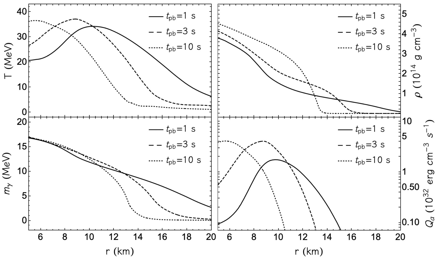
In Fig. 2 we show the axion emissivity as a function of the SN radius at different post-bounce times (bottom right panel), together with the physical properties which determine it, namely the temperature (upper left panel), the matter density g cm-3 (upper right panel) and the effective photon mass MeV in the core (bottom left panel). In particular, at s, the production zone is at km and it moves towards the star center at larger times, reflecting the behaviour of the peak temperature MeV and showing the strong temperature dependence of the production rate. The axion energy luminosity, i.e. the energy emitted by axions per unit time, is obtained by integrating the emissivity over the stellar volume, i.e.
| (12) |
We mention that redshift corrections need to be considered in order to evaluate the luminosity for a distant observer, as discussed in Refs. [56, 57]. Indeed, after its emission, an axion will suffer a gravitational redshift before reaching an observer at infinity. This effect is encoded in the “lapse” factor listed at each radius in the SN simulation data [52]. This means that the observed axion energy at infinity is , where is the axion energy in the local comoving frame of reference, in which SN-simulation data are provided. In addition, for the rate of emission another redshift correction is required, since the proper time lapse of a comoving observer is related to the distant observer time by the lapse function [52]. Therefore, the contribution from local emission to the luminosity at infinity can be evaluated by including a factor . Moreover, since all physical properties of the star are given in the comoving reference frame of the emitting medium, a Doppler shift effect has to be considered, where is the radial velocity of the medium, which is always very small [56, 57]. For this reason, the observed axion luminosity at infinity is given by
| (13) |
where is the emission rate evaluated in the local comoving frame of reference. We stress again that since , the last term in brackets has a small impact on the observed luminosity, while the factor reduces the luminosity by a factor , in agreement with Ref. [56].
III SN 1987A cooling bound
The observation of the SN 1987A neutrino burst permits to constrain all the exotic energy losses that would significantly shorten its duration. For quantitative estimates, it is normally assumed that the luminosity associated with exotic processes, calculated at a representative time s after the core-bounce, does not exceed the neutrino luminosity erg s-1 [58, 56]. In order to place a bound on the axion coupling , we evaluate the axion luminosity adopting the “modified luminosity criterium”, (see [59, 60, 56])
| (14) |
where the integral of the axion emissivity is performed on the emission region with km and the exponential suppression takes into account the possibility of axion absorption. In particular, is a directional average of the absorption factor
| (15) |
where is the axion mean-free path calculated in Eq. (71) in Appendix B, is the axion redshifted energy, and is the angle between the outward radial direction and a given ray of propagation along which is integrated.
In Fig. 3, we show the expected bound on in the vs plane. The trend is a typical one often discussed in literature (see, e.g., Ref. [58]). The region for corresponds to the free-streaming case, where the axion production is dominated by a volume emission and . Conversely, for axions enter the trapping regime, where the luminosity is dominated by a surface black-body emission from an “axion-sphere” with radius , where that is a rapidly decreasing function of so that decreases when increases. We exclude values of for which erg s-1, corresponding to the range . We notice that the bound on in the free-streaming regime is slightly weaker than the simple back-of-the-envelope estimation presented in Ref. [38], namely GeV-2. Furthermore, as shown in Sec. V, values of larger than what excluded by the trapping limit are excluded by the extra radiation produced by the thermalization of axions in the early Universe. Therefore, in the next section we will focus on couplings below the free-streaming bound.
IV Axion signal in Hyper-Kamiokande
Having calculated the SN axion spectrum produced through the nucleon dipole portal, our goal in this section is to discuss detection possibilities from a Galactic SN explosion with next generation neutrino detectors (see, e.g., Ref. [61] for a review). For definiteness, we focus on the neutrino underground water Cherenkov detector Hyper-Kamiokande, with a proposed fiducial mass of 374 kton [46]. In this case the detection channel is the scattering of the SN axions on free protons in the water
| (16) |
producing a visible photon flux. In order to calculate the event rate in Hyper-Kamiokande, one has to consider the SN axion fluence from Eq. (10), including gravitational redshift. This is well-represented by the following quasi-thermal spectrum (see also [62])
| (17) |
where , and . This spectrum is shown in Fig. 4 for GeV-1 and negligible axion mass.
The detection cross section, associated with the process in Eq. (16), is given by
| (18) |
where in the last step we used the small axion mass limit and the non-relativistic approximation for nucleons, so that and , subject to the kinematical constraint
| (19) |
The produced photon energy spectrum is given by
| (20) |
where is the SN distance from Earth, and is the number of targets in the detector,
| (21) |
with the number of free protons per water molecule, the Avogadro number and g/mol the molar mass of water.
In Fig. 5, we show the event rate in Hyper-Kamiokande for the axion signal via (continuous curve) and for a Galactic SN at kpc, representative of the distance of the red supergiant star Betelgeuse [63]. For comparison, we show the neutrino event rate associated with inverse beta decay process, (dashed curve) which is the dominant detection channel for SN neutrinos (see, e.g., Ref. [64]). It is interesting to realize that for MeV, the axion signal emerges over the background, offering a potential window of detection. The high-statistics SN neutrino detection can be used as an external trigger for the axion detection. Indeed, it selects a s time window to look at the coincidence of at least two photons from axions signal. Notably, the accidental background coincidence in a 10 s window is small, less than one event every three years.33 3 Mark Vagins, private communication. The number of axion events for MeV is given by
| (22) |
In Fig. 6, we show the number of expected events in Hyper-Kamiokande as a function of , for different values of the SN distance. It is apparent that a few hundreds of events would be detected for GeV-2 near the cooling bound and for a SN explosion at distance kpc, such as Betelgeuse. Distances up to kpc would give a handful of events for the same value of the coupling. For a close-by SN at kpc, we expect to observe few events for couplings larger than GeV-2. In order to quantify the sensitivity to as a function of the SN distance , in Fig. 7 we show the Poisson probability to detect more than two photon events with MeV in Hyper-Kamiokande as a function of the SN distance, for three different values of the coupling, evaluated as
| (23) |
We see that for GeV-2, there is a non-negligible probability () to detect an axion-signal up to 2.5 kpc. For GeV-2, the sensitivity radius is reduced to 1 kpc, and for GeV-2 to 300 pc. There are SN candidates in a radius kpc [65]. According to our analysis, if one of these goes SN we might expect, together with a huge neutrino signal, a handful of high-energy events associated with the nucleon dipole portal to axions.
V Cosmological bounds on axion extra radiation
A complementary constraint on the axion nucleon dipole portal can be derived from measurements of extra radiation in the early universe. In fact, below the QCD phase transition, the process becomes an effective process to produce a thermal population of axions which would contribute to extra radiation. The axion production rate in the early Universe is given by where is the nucleon thermal number density and the production cross section is given by Eq. (18). Axions decouple when , where is the Universe Hubble expansion rate. Having determined the axion decoupling temperature , it is possible to calculate the effective number of relativistic degrees of freedom, appearing as extra radiation, as [66, 2]
| (24) |
where are the entropic effective degrees of freedom (normalized to the total number of SM degrees of freedom). The sensitivity of the Planck 2018 data is enough to exclude at CL [67], which corresponds to . Therefore, the cosmological bound nicely connects with the exclusion given by the SN 1987A in the trapping regime. We remark that, for eV, axions would be too heavy to be considered dark radiation and their constraint from contributing to dark matter is much weaker than the one from .
For values below the SN 1987A bound in the free-streaming regime, , axions would decouple before the QCD phase transition. In this case the processes relevant for their thermalization are the ones with gluons, rather than with nucleons. In this case the decoupling temperature can be estimated as [2] (see also [30, 31, 32, 33, 34, 35, 36]), which is typically well above the electroweak scale. Hence, from Eq. (24) it follows that , which is in the reach of future CMB-S4 surveys [68]. Requiring that the temperature of the Universe was high enough to bring the axion into thermal equilibrium, , CMB-S4 data would be able to probe [33]
| (25) |
VI Discussion and Conclusions
In this work, we provided a careful quantitative investigation of the bounds and signatures of a nucleon dipole portal to axions from a SN explosion. First, we have revised the axion production channels in a SN. The most relevant channels are the Compton and the bremsstrahlung processes, the last of which had never been considered in the previous literature. We present a detailed calculation of the rates associated with both processes in Appendix C. We find that the SN 1987A cooling argument provides the limit . Furthermore, we have shown that for values of below this bound and larger than a future Galactic SN explosion within a radius kpc would produce a handful of events through the process in the Hyper-Kamiokande detector.
In the case of QCD axion, Eq. (4) holds and the bound on can be translated into GeV. However, we stress that in this case the SN bound on due to nucleon-EDM coupling would be weaker than the HB bound due to axion-photon coupling ( GeV) [69] and the SN bound due to axion-nucleon couping ( GeV) [23]. Therefore, the nucleon-EDM axion coupling would be the most important one for axion phenomenology only in the case in which both photon- and nucleon- axion couplings are suppressed. As further discussed in Appendix A, the required cancellation cannot be achieved with only a single tuning, but further non-trivial assumptions are needed.
It is interesting to compare the axion parameter space probed by SNe with sensitivities of other searches in the plane , as shown in the upper panel of Fig. 8. There, the shaded green area is excluded by the non-detection of an oscillating nuclear dipole moment in experiments looking for a static one (nEDM, see [70]). The dashed lines represent future sensitivity estimates for different phases of the oscillating EDM experiment CASPERe [29]. Our SN 1987A bound is the blue shaded strip between . Higher values of the coupling are excluded by extra radiation produced after the QCD phase transition. Values (dashed curve) can be probed by axion events from a future close-by Galactic SN explosion.
In the lower panel of Fig. 8, we superimpose additional bounds and future sensitivities under the assumption that the origin of is the anomalous axion-gluon coupling, depending on in the case of the QCD axion (oblique yellow band) [see Eqs. (2)–(4)]. The region below the dotted grey line () corresponds to , while in the grey region (BBN) axions coupled to QCD are inconsistent with the production of the observed abundance of light elements during Big Bang Nucleosynthesis (BBN) [71]. Note that both CASPERe and the BBN bound rely on the assumption that the axion comprises the whole cold dark matter. Instead, the bounds denoted as ‘‘Earth’’ and ‘‘Sun’’ are due to finite density effects. In fact, in models where the axion mass is down-tuned,44 4 In the presence of an extra dark sector contributing to the axion mass, the latter can be suppressed with respect to the value set by QCD. In some studies (e.g. [71, 72]) this was supposed to happen via a tuning. More recently, exploiting the mechanism proposed in [73], Refs. [74, 75] showed that the axion mass can be exponentially suppressed in terms of a symmetry, while solving the strong CP problem and the axion being dark matter. These works motivate the region on the left of the “QCD axion band” in Fig. 8. the cancellation of the axion mass can be spoiled in high-density stellar environments where the axion field relaxes to , implying various experimental constraints (see Ref. [76] for more details). The shaded grey region around eV represents the most conservative Black-Hole superradiance bound [77] (but see also Ref. [78]). Finally, if axions decouple before the QCD phase transition, e.g. via the axion-gluon coupling, their contribution to extra radiation would be in the reach of future CMB-S4 observations [68], improving over existing constraints on . In the lower panel of Fig. 8 we show what the reach in would be, assuming a reheating temperature of GeV.
We notice that the region probed by CMB-S4 is complementary to the direct search of axion dark matter by the CASPERe experiment [29]. Remarkably, also our SN signal is complementary with CASPERe. Indeed, for masses eV, if one would not observe any signal in CASPERe, but there is the possibility to get a few axion-induced events from a close-by SN and an excess of extra radiation in CMB-S4. This is a peculiar scenario where the nucleon dipole portal would be invisible to laboratory experiments and would show up only from the sky.
Acknowledgements.
We warmly thank Andreas Ringwald for interesting discussions stimulating this project. AM warmly thanks Mark Vagins for useful discussions on Hyper-Kamiokande during the development of this project. The work of GL and AM is partially supported by the Italian Istituto Nazionale di Fisica Nucleare (INFN) through the “Theoretical Astroparticle Physics” project and by the research grant number 2017W4HA7S “NAT-NET: Neutrino and Astroparticle Theory Network” under the program PRIN 2017 funded by the Italian Ministero dell’Università e della Ricerca (MUR). The work of PC is supported by the European Research Council under Grant No. 742104 and by the Swedish Research Council (VR) under grants 2018-03641 and 2019-02337. The work of LDL is partially supported by the European Union’s Horizon 2020 research and innovation programme under the Marie Skłodowska-Curie grant agreement No 860881 - HIDDEN. The work of LM is supported by the Italian Istituto Nazionale di Fisica Nucleare (INFN) through the “QGSKY” project and by Ministero dell’Istruzione, Università e Ricerca (MIUR).Appendix A QCD axions with suppressed couplings to photons and matter fields
In this Appendix, we explore the question of whether it is possible to conceive a QCD axion model where the nucleon-EDM portal provides the leading axion interaction. This requires in turn that standard axion couplings to photons and matter fields are suppressed with respect to their natural values.
To formulate the problem in general terms, let us start from the axion effective Lagrangian below the electroweak scale
| (26) |
where is the ratio of the QED/QCD anomaly of the PQ current and denotes SM Dirac fermions. The ellipses in Eq. (A) stand for extra terms like off-diagonal fermion currents, including vector ones. This Lagrangian is matched with the axion effective Lagrangian below the scale of chiral symmetry breaking, GeV, which reads
| (27) |
where we kept only terms that are relevant for axion phenomenology, namely nucleons (), pions, electrons and photons. In fact, the axion-pion coupling is relevant for the axion hot dark matter bound through to axion-pion thermalization channel [79, 80, 81] while the other couplings are constrained by astrophysical considerations. The Wilson coefficients of the two effective Lagrangians in Eqs. (A)-(A) are related as follows (see e.g. [2])
| (28) | ||||
| (29) | ||||
| (30) | ||||
| (31) | ||||
| (32) | ||||
| (33) |
where , , and [82]. Here, we neglected corrections coming from flavour mixing as well as radiative corrections (see below).
The condition that we want to impose corresponds to
| (34) |
such that axion phenomenology is driven by the nucleon EDM couplings. From an effective field theory point of view the couplings in Eqs. (29)-(33) should be regarded as free parameters and hence it is conceivably possible that they are suppressed with respect to the values suggested by benchmark axion models.
Here, we want to provide a proof of existence of a UV completion that can realize the conditions in Eq. (34). To this end, we start from the non-universal axion model of Ref. [83], which can realize the nucleo/pion/electro-phobic conditions
| (35) |
at the price of a single tuning. The model extends the scalar sector of the SM with three Higgs doublets and a SM singlet . The scalar potential features the non-Hermitian SM invariant operators
| (36) |
which imply the conditions (normalizing to the unity the PQ charge of , i.e. )
| (37) | ||||
| (38) | ||||
| (39) |
where the latter condition arises from the orthogonality between the PQ and hypercharge currents, with and the square of the Higgs vacuum expectation value. The Yukawa sector features the following operators, with a non-universal assignment of the PQ charges in the quark sector with a 2+1 structure (i.e. first and second family, denoted by greek indices, are characterized by the same PQ charge)
| (40) | |||
| (41) |
with . Differently from Ref. [83], that assumed a universal PQ charge assignment in the lepton sector, in order to obtain here a suppressed coupling to photons (see below) we assume
| (42) |
Neglecting flavour mixing,55 5 In the presence of flavour mixing, , where involves off-diagonal elements of fermion mass diagonalization matrices, which are assumed here to be negligible. See Refs. [84, 85] for details. the flavour diagonal axion couplings to the axial current read
| (43) | ||||
| (44) | ||||
| (45) |
where we used the value of the QCD anomaly factor given by
| (46) |
and we also used Eqs. (37)-(38). Since, by construction, we have
| (47) |
then Eq. (29) implies (up to corrections from ). On the other hand, the condition requires the tuning (see Eq. (30))
| (48) |
that is
| (49) |
where in the second step we used Eqs. (37)-(38). Note that this condition (satisfied for ) also automatically guarantees (see Eq. (31)) and (see Eq. (32) and Eq. (A)). Defining the vacuum angles via
| (50) | ||||
| (51) | ||||
| (52) |
we can express
| (53) |
and parametrize the couplings above in terms of the vacuum angles that are subject to perturbative unitarity constraints (see Ref. [83]).
Finally, the QED anomaly factor can be split into a quark plus lepton contribution, i.e. , which read respectively
| (54) | ||||
| (55) |
and hence , corresponding to the photo-phobic coupling .
In summary, the model is characterized by the following axion couplings:
| (56) | ||||
| (57) | ||||
| (58) | ||||
| (59) | ||||
| (60) | ||||
| (61) |
The condition in Eq. (34) is hence obtained at the prize of a single tuning, i.e. , where can be expressed in terms of vacuum angles of the extended Higgs sector, see Eq. (53). In particular, is obtained for which is fully within the perturbative domain of the model (see Ref. [83]). We remark that the advocated level of suppression of axion couplings can be kept also upon including running effects from to the QCD scale, albeit within fairly different parameter space regions than in the tree-level case [86]
On the other hand, the level of cancellation that can be achieved in the model above (for ) is not yet sufficient to make the nucleon-EDM axion coupling the most important one for axion phenomenology. Indeed, the two strongest astrophysical constraints on are due to and , coming from HB stars [69] and SNe [23], respectively. An order of magnitude suppression in is sufficient to evade the former, while the latter is a factor stronger than the SN bound due to nucleon-EDM coupling. Therefore the suppression proposed in the model in Eqs. (56)-(61) is enough to evade the HB bound but not sufficient for the SN bound due to . Hence a further order of magnitude cancellation in would be required. This can be achieved at the price of extra tunings. For instance, can be further suppressed by taking into account flavour mixing effects for flavour-diagonal axion couplings (see Refs. [84, 85] for details), while can be modified via an extra KSVZ-like fermionic sector along the lines of [87, 88] which contributes to the electromagnetic anomaly.
We conclude that although a percent level suppression of axion couplings seems perfectly feasible in explicit QCD axion models, going below that level requires further non-trivial assumptions.
Appendix B Evaluation of the emissivity and absorption mean free path
The axion emissivity due to Compton scattering is given by
| (62) |
where is given by Eq. (6), , , and are the 4-momenta of the initial and final state nucleon , the photon and the axion, respectively. In addition, ’s are the usual Fermi-Dirac or Bose-Einstein distributions, i.e.
| (63) |
where the sign applies to fermions, the is for bosons, and are the chemical potentials for , while photons have vanishing chemical potential. Following Ref. [54], the integration in Eq. (62) can be simplified and the emissivity is given by
| (64) |
where , , and
| (65) |
with the angle between the axion and the photon momenta, and , , , given by
| (66) |
where the constants , , are
| (67) |
The integration domain for is composed by and , with and
| (68) |
Finally, we stress that in the case of interest , since we are considering light axions ().
On the other hand, axions may be absorbed due to the inverse process . The absorption mean free path is
| (69) |
where is the nucleon density and is the absorption cross section given by
| (70) |
This expression differs from Eq. (62) due to the absence of the integration over the axion energy, i.e. , and the interchange between the initial and final states. Therefore, following once more Ref. [54], one obtains
| (71) |
Appendix C Emissivities in the non-degenerate and non-relativistic limit
C.1 Compton effect
In order to obtain a simple expression for the Compton emissivity, let us evaluate it in the non-degenerate and non-relativistic limit for nucleons, ignoring also the effective photon mass. The general expression for the emissivity is
| (72) |
where , , , and are the 4-momenta of the initial and final state nucleon , the photon and the axion, respectively, with , and . In addition, all the ’s are considered as Maxwell-Boltzmann distributions, i.e.
| (73) |
where are the chemical potentials for nucleons, while photons and axions have vanishing chemical potential. In the non degenerate limit the Pauli blocking factors are negligible, , and we can approximate
| (74) |
To further simplify the expression, let us fix as reference system the center of momentum frame, in which and . We can integrate over to eliminate , obtaining a constraint on , since
| (75) |
and rewrite the transition matrix as
| (76) |
being . Since , and , we obtain
| (77) | |||||
Integrating over , and exploiting the relation in the non-degenerate and non-relativistic limit
| (78) |
we obtain
| (79) | |||||
Now, using the relations and , we conclude that
| (80) |
We are considering both the contributions of protons and neutron , then the emissivity per unit mass can be written in the following form
For typical SN conditions ( g cm-3, MeV, ), imposing the cooling bound erg g-1 s-1, the coupling is constrained to be GeV-2, in rough agreement with the estimation in Ref. [38].
C.2 Bremsstrahlung
In this Section, we evaluate the bremsstrahlung emissivity in the non-relativistic and non-degenerate approximation for nucleons, which is thought to be a good approximation in a SN core, and we show that this process is subdominant with respect to the Compton emission for typical SN conditions.
In the bremsstrahlung process, an axion is produced after the interaction between a nucleon () and a virtual photon emitted by a proton (). We classify the bremsstrahlung as channel if (see Fig. 9) and channel if (see Fig. 10). Therefore the emissivity is given by the sum of the two channels
| (82) |
where is due to process and is due to the channel. Let us start from the process. In this case the emissivity is given by


| (83) | |||||
with
| (84) |
where we are averaging the nucleon spins of the initial and final states and the matrix element is (see Fig. 9)
| (85) |
being the electric charge, the transferred-photon 4-momentum and the metric tensor. Assuming that nucleons are non-relativistic and non-degenerate, , we can write
| (86) | |||||
where
| (87) |
with , and and . In addition, due to the non-relativistic approximation
| (88) | |||
Following Refs. [53, 89, 90, 91] let us introduce the center-of-momentum variables
| (89) |
In the non-relativistic limit, a typical nucleon with kinetic energy has momentum . Then, the three dimensional delta function implies . Due to the non relativistic approximation
| (90) |
and using Eq. (89) , we obtain
| (91) | |||||
Then, given , , , , the squared matrix element can be written in terms of the new variables as
| (92) | |||||
and
| (93) |
One can introduce the variables
| (94) |
then the delta function in Eq. (86) can be rewritten as
| (95) |
and we integrate over using the three-dimensional piece. We now change the integration variables where is due to the Jacobian, and using
| (96) | |||||
we obtain
| (97) |
where we fix due to the -function and
| (98) |
The -channel contribution (see Fig. 10) is given by
| (99) | |||||
where
| (100) |
being
| (101) |
with the direct-diagram contribution (upper left panel in Fig. 10) and the exchange-diagram, obtained interchanging the final fermion lines (upper right panel in Fig. 10). In Eq. (62), is the symmetry factor
| (102) |
where comes from the position where the axion can be attached (upper or lower vertex, see the lower panels of Fig. 10), and comes from the identical particles in the initial and final states (for the process ). Assuming non-relativistic and non-degenerate nucleons, the matrix element in Eq. (101) can be evaluated following a procedure analogous to the process and the -contribution reads as
| (103) |
which differs from Eq. (97) due to the replacements (since only protons are involved), in the denominator (due to the symmetry factor ) and , where
| (104) |
The total emissivity in Eq. (82) is obtained summing Eqs. (97) and (103). Assuming typical SN conditions ( g cm-3, MeV, ), the emissivity per unit mass erg g-1 s-1 , more than one order of magnitude smaller than the Compton emissivity [see Eq. ()], in agreement with other cases discussed in literature (see e.g. Sec. II C in Ref. [56]).
References
- [1] J. Jaeckel and A. Ringwald, The Low-Energy Frontier of Particle Physics, Ann. Rev. Nucl. Part. Sci. 60 (2010) 405 [1002.0329].
- [2] L. Di Luzio, M. Giannotti, E. Nardi and L. Visinelli, The landscape of QCD axion models, Phys. Rept. 870 (2020) 1 [2003.01100].
- [3] S. Weinberg, A New Light Boson?, Phys. Rev. Lett. 40 (1978) 223.
- [4] F. Wilczek, Problem of Strong and Invariance in the Presence of Instantons, Phys. Rev. Lett. 40 (1978) 279.
- [5] R. D. Peccei and H. R. Quinn, CP Conservation in the Presence of Instantons, Phys. Rev. Lett. 38 (1977) 1440.
- [6] R. D. Peccei and H. R. Quinn, Constraints Imposed by CP Conservation in the Presence of Instantons, Phys. Rev. D 16 (1977) 1791.
- [7] E. Masso, F. Rota and G. Zsembinszki, Planck-scale effects on global symmetries: Cosmology of pseudo-Goldstone bosons, Phys. Rev. D 70 (2004) 115009 [hep-ph/0404289].
- [8] A. Arvanitaki, S. Dimopoulos, S. Dubovsky, N. Kaloper and J. March-Russell, String axiverse, Phys. Rev. D 81 (2010) 123530 [0905.4720].
- [9] M. Cicoli, M. Goodsell and A. Ringwald, The type IIB string axiverse and its low-energy phenomenology, JHEP 10 (2012) 146 [1206.0819].
- [10] I. Broeckel, M. Cicoli, A. Maharana, K. Singh and K. Sinha, Moduli stabilisation and the statistics of axion physics in the landscape, JHEP 08 (2021) 059 [2105.02889].
- [11] J. Preskill, M. B. Wise and F. Wilczek, Cosmology of the invisible axion, Phys. Lett. B 120 (1983) 127.
- [12] L. F. Abbott and P. Sikivie, A cosmological bound on the invisible axion, Phys. Lett. B 120 (1983) 133.
- [13] M. Dine and W. Fischler, The Not So Harmless Axion, Phys. Lett. B 120 (1983) 137.
- [14] G. Raffelt and L. Stodolsky, Mixing of the photon with low mass particles, Phys. Rev. D 37 (1988) 1237.
- [15] I. G. Irastorza and J. Redondo, New experimental approaches in the search for axion-like particles, Prog. Part. Nucl. Phys. 102 (2018) 89 [1801.08127].
- [16] P. Sikivie, Invisible Axion Search Methods, Rev. Mod. Phys. 93 (2021) 015004 [2003.02206].
- [17] G. G. Raffelt, Astrophysical axion bounds diminished by screening effects, Phys. Rev. D 33 (1986) 897.
- [18] G. G. Raffelt, Astrophysical axion bounds, Lect. Notes Phys. 741 (2008) 51 [hep-ph/0611350].
- [19] L. Di Luzio, M. Fedele, M. Giannotti, F. Mescia and E. Nardi, Stellar evolution confronts axion models, JCAP 02 (2022) 035 [2109.10368].
- [20] P. Carenza and G. Lucente, Revisiting axion-electron bremsstrahlung emission rates in astrophysical environments, Phys. Rev. D 103 (2021) 123024 [2104.09524].
- [21] A. Burrows, M. S. Turner and R. P. Brinkmann, Axions and SN 1987a, Phys. Rev. D 39 (1989) 1020.
- [22] A. Burrows, M. T. Ressell and M. S. Turner, Axions and SN1987A: Axion trapping, Phys. Rev. D 42 (1990) 3297.
- [23] P. Carenza, T. Fischer, M. Giannotti, G. Guo, G. Martínez-Pinedo and A. Mirizzi, Improved axion emissivity from a supernova via nucleon-nucleon bremsstrahlung, JCAP 10 (2019) 016 [1906.11844]. [Erratum: JCAP 05, E01 (2020)].
- [24] P. Carenza, M. Lattanzi, A. Mirizzi and F. Forastieri, Thermal axions with multi-eV masses are possible in low-reheating scenarios, JCAP 07 (2021) 031 [2104.03982].
- [25] T. Fischer, P. Carenza, B. Fore, M. Giannotti, A. Mirizzi and S. Reddy, Observable signatures of enhanced axion emission from protoneutron stars, Phys. Rev. D 104 (2021) 103012 [2108.13726].
- [26] A. Arvanitaki and A. A. Geraci, Resonantly Detecting Axion-Mediated Forces with Nuclear Magnetic Resonance, Phys. Rev. Lett. 113 (2014) 161801 [1403.1290].
- [27] R. Barbieri, C. Braggio, G. Carugno, C. S. Gallo, A. Lombardi, A. Ortolan, R. Pengo, G. Ruoso and C. C. Speake, Searching for galactic axions through magnetized media: the QUAX proposal, Phys. Dark Univ. 15 (2017) 135 [1606.02201].
- [28] N. Crescini, C. Braggio, G. Carugno, P. Falferi, A. Ortolan and G. Ruoso, Improved constraints on monopole-dipole interaction mediated by pseudo-scalar bosons, Phys. Lett. B 773 (2017) 677 [1705.06044].
- [29] D. F. Jackson Kimball et al., Overview of the Cosmic Axion Spin Precession Experiment (CASPEr), Springer Proc. Phys. 245 (2020) 105 [1711.08999].
- [30] E. Masso, F. Rota and G. Zsembinszki, On axion thermalization in the early universe, Phys. Rev. D 66 (2002) 023004 [hep-ph/0203221].
- [31] P. Graf and F. D. Steffen, Thermal axion production in the primordial quark-gluon plasma, Phys. Rev. D83 (2011) 075011 [1008.4528].
- [32] A. Salvio, A. Strumia and W. Xue, Thermal axion production, JCAP 1401 (2014) 011 [1310.6982].
- [33] D. Baumann, D. Green and B. Wallisch, New Target for Cosmic Axion Searches, Phys. Rev. Lett. 117 (2016) 171301 [1604.08614].
- [34] F. D’Eramo, F. Hajkarim and S. Yun, Thermal Axion Production at Low Temperatures: A Smooth Treatment of the QCD Phase Transition, Phys. Rev. Lett. 128 (2022) 152001 [2108.04259].
- [35] F. D’Eramo, F. Hajkarim and S. Yun, Thermal QCD Axions across Thresholds, JHEP 10 (2021) 224 [2108.05371].
- [36] W. Giarè, F. Renzi, A. Melchiorri, O. Mena and E. Di Valentino, Cosmological forecasts on thermal axions, relic neutrinos, and light elements, Mon. Not. Roy. Astron. Soc. 511 (2022) 1373 [2110.00340].
- [37] T. Altherr, Plasmon effects in light scalar and pseudoscalar emission from a supernova, Annals Phys. 207 (1991) 374.
- [38] P. W. Graham and S. Rajendran, New Observables for Direct Detection of Axion Dark Matter, Phys. Rev. D 88 (2013) 035023 [1306.6088].
- [39] M. Pospelov and A. Ritz, Theta induced electric dipole moment of the neutron via QCD sum rules, Phys. Rev. Lett. 83 (1999) 2526 [hep-ph/9904483].
- [40] D. Budker, P. W. Graham, M. Ledbetter, S. Rajendran and A. Sushkov, Proposal for a Cosmic Axion Spin Precession Experiment (CASPEr), Phys. Rev. X 4 (2014) 021030 [1306.6089].
- [41] Y. V. Stadnik and V. V. Flambaum, Axion-induced effects in atoms, molecules, and nuclei: Parity nonconservation, anapole moments, electric dipole moments, and spin-gravity and spin-axion momentum couplings, Phys. Rev. D 89 (2014) 043522 [1312.6667].
- [42] V. V. Flambaum, M. Pospelov, A. Ritz and Y. V. Stadnik, Sensitivity of EDM experiments in paramagnetic atoms and molecules to hadronic CP violation, Phys. Rev. D 102 (2020) 035001 [1912.13129].
- [43] T. S. Roussy et al., Experimental Constraint on Axionlike Particles over Seven Orders of Magnitude in Mass, Phys. Rev. Lett. 126 (2021) 171301 [2006.15787].
- [44] Kamiokande-II Collaboration, K. Hirata et al., Observation of a Neutrino Burst from the Supernova SN 1987a, Phys. Rev. Lett. 58 (1987) 1490.
- [45] R. M. Bionta et al., Observation of a Neutrino Burst in Coincidence with Supernova SN 1987a in the Large Magellanic Cloud, Phys. Rev. Lett. 58 (1987) 1494.
- [46] K. Abe et al., Letter of Intent: The Hyper-Kamiokande Experiment — Detector Design and Physics Potential —, 1109.3262.
- [47] P. Carenza, B. Fore, M. Giannotti, A. Mirizzi and S. Reddy, Enhanced Supernova Axion Emission and its Implications, Phys. Rev. Lett. 126 (2021) 071102 [2010.02943].
- [48] A. Kopf and G. Raffelt, Photon dispersion in a supernova core, Phys. Rev. D 57 (1998) 3235 [astro-ph/9711196].
- [49] M. Hempel, Nucleon self-energies for supernova equations of state, Phys. Rev. C 91 (2015) 055807 [1410.6337].
- [50] G. Martinez-Pinedo, T. Fischer, A. Lohs and L. Huther, Charged-current weak interaction processes in hot and dense matter and its impact on the spectra of neutrinos emitted from proto-neutron star cooling, Phys. Rev. Lett. 109 (2012) 251104 [1205.2793].
- [51] A. Mezzacappa and S. Bruenn, A numerical method for solving the neutrino Boltzmann equation coupled to spherically symmetric stellar core collapse, Astrophys. J. 405 (1993) 669.
- [52] M. Liebendoerfer, O. E. B. Messer, A. Mezzacappa, S. W. Bruenn, C. Y. Cardall and F. K. Thielemann, A Finite difference representation of neutrino radiation hydrodynamics for spherically symmetric general relativistic supernova simulations, Astrophys. J. Suppl. 150 (2004) 263 [astro-ph/0207036].
- [53] R. P. Brinkmann and M. S. Turner, Numerical Rates for Nucleon-Nucleon Axion Bremsstrahlung, Phys. Rev. D 38 (1988) 2338.
- [54] S. Hannestad and J. Madsen, Neutrino decoupling in the early universe, Phys. Rev. D 52 (1995) 1764 [astro-ph/9506015].
- [55] L. Mastrototaro, P. D. Serpico, A. Mirizzi and N. Saviano, Massive sterile neutrinos in the early Universe: From thermal decoupling to cosmological constraints, Phys. Rev. D 104 (2021) 016026 [2104.11752].
- [56] A. Caputo, G. Raffelt and E. Vitagliano, Muonic boson limits: Supernova redux, Phys. Rev. D 105 (2022) 035022 [2109.03244].
- [57] A. Caputo, H.-T. Janka, G. Raffelt and E. Vitagliano, Low-Energy Supernovae Severely Constrain Radiative Particle Decays, 2201.09890.
- [58] G. Raffelt and D. Seckel, Bounds on Exotic Particle Interactions from SN 1987a, Phys. Rev. Lett. 60 (1988) 1793.
- [59] J. H. Chang, R. Essig and S. D. McDermott, Revisiting Supernova 1987A Constraints on Dark Photons, JHEP 01 (2017) 107 [1611.03864].
- [60] G. Lucente, P. Carenza, T. Fischer, M. Giannotti and A. Mirizzi, Heavy axion-like particles and core-collapse supernovae: constraints and impact on the explosion mechanism, JCAP 12 (2020) 008 [2008.04918].
- [61] A. Mirizzi, I. Tamborra, H.-T. Janka, N. Saviano, K. Scholberg, R. Bollig, L. Hudepohl and S. Chakraborty, Supernova Neutrinos: Production, Oscillations and Detection, Riv. Nuovo Cim. 39 (2016) 1 [1508.00785].
- [62] A. Payez, C. Evoli, T. Fischer, M. Giannotti, A. Mirizzi and A. Ringwald, Revisiting the SN1987A gamma-ray limit on ultralight axion-like particles, JCAP 02 (2015) 006 [1410.3747].
- [63] G. M. Harper, A. Brown, E. F. Guinan, E. O’Gorman, A. M. S. Richards, P. Kervella and E.-m. g. Decin, L., An updated 2017 astrometric solution for betelgeuse, Astronomical Journal (New York, N.Y. Online) 154 (2017) .
- [64] G. L. Fogli, E. Lisi, A. Mirizzi and D. Montanino, Probing supernova shock waves and neutrino flavor transitions in next-generation water-Cerenkov detectors, JCAP 04 (2005) 002 [hep-ph/0412046].
- [65] M. Mukhopadhyay, C. Lunardini, F. X. Timmes and K. Zuber, Presupernova neutrinos: directional sensitivity and prospects for progenitor identification, Astrophys. J. 899 (2020) 153 [2004.02045].
- [66] E. W. Kolb and M. S. Turner, The Early Universe, Nature 294 (1981) 521.
- [67] Planck Collaboration, N. Aghanim et al., Planck 2018 results. VI. Cosmological parameters, Astron. Astrophys. 641 (2020) A6 [1807.06209]. [Erratum: Astron.Astrophys. 652, C4 (2021)].
- [68] K. Abazajian et al., CMB-S4 Science Case, Reference Design, and Project Plan, 1907.04473.
- [69] A. Ayala, I. Domínguez, M. Giannotti, A. Mirizzi and O. Straniero, Revisiting the bound on axion-photon coupling from Globular Clusters, Phys. Rev. Lett. 113 (2014) 191302 [1406.6053].
- [70] C. Abel et al., Search for Axionlike Dark Matter through Nuclear Spin Precession in Electric and Magnetic Fields, Phys. Rev. X 7 (2017) 041034 [1708.06367].
- [71] K. Blum, R. T. D’Agnolo, M. Lisanti and B. R. Safdi, Constraining Axion Dark Matter with Big Bang Nucleosynthesis, Phys. Lett. B 737 (2014) 30 [1401.6460].
- [72] G. Alonso-Álvarez and J. Jaeckel, Exploring axionlike particles beyond the canonical setup, Phys. Rev. D 98 (2018) 023539 [1712.07500].
- [73] A. Hook, Solving the Hierarchy Problem Discretely, Phys. Rev. Lett. 120 (2018) 261802 [1802.10093].
- [74] L. Di Luzio, B. Gavela, P. Quilez and A. Ringwald, An even lighter QCD axion, JHEP 05 (2021) 184 [2102.00012].
- [75] L. Di Luzio, B. Gavela, P. Quilez and A. Ringwald, Dark matter from an even lighter QCD axion: trapped misalignment, JCAP 10 (2021) 001 [2102.01082].
- [76] A. Hook and J. Huang, Probing axions with neutron star inspirals and other stellar processes, JHEP 06 (2018) 036 [1708.08464].
- [77] M. Baryakhtar, M. Galanis, R. Lasenby and O. Simon, Black hole superradiance of self-interacting scalar fields, Phys. Rev. D 103 (2021) 095019 [2011.11646].
- [78] V. M. Mehta, M. Demirtas, C. Long, D. J. E. Marsh, L. Mcallister and M. J. Stott, Superradiance Exclusions in the Landscape of Type IIB String Theory, 2011.08693.
- [79] S. Chang and K. Choi, Hadronic axion window and the big bang nucleosynthesis, Phys. Lett. B 316 (1993) 51 [hep-ph/9306216].
- [80] S. Hannestad, A. Mirizzi and G. Raffelt, New cosmological mass limit on thermal relic axions, JCAP 07 (2005) 002 [hep-ph/0504059].
- [81] L. Di Luzio, G. Martinelli and G. Piazza, Breakdown of chiral perturbation theory for the axion hot dark matter bound, Phys. Rev. Lett. 126 (2021) 241801 [2101.10330].
- [82] G. Grilli di Cortona, E. Hardy, J. Pardo Vega and G. Villadoro, The QCD axion, precisely, JHEP 01 (2016) 034 [1511.02867].
- [83] F. Björkeroth, L. Di Luzio, F. Mescia, E. Nardi, P. Panci and R. Ziegler, Axion-electron decoupling in nucleophobic axion models, Phys. Rev. D 101 (2020) 035027 [1907.06575].
- [84] L. Di Luzio, F. Mescia, E. Nardi, P. Panci and R. Ziegler, Astrophobic Axions, Phys. Rev. Lett. 120 (2018) 261803 [1712.04940].
- [85] F. Björkeroth, L. Di Luzio, F. Mescia and E. Nardi, flavour symmetries as Peccei-Quinn symmetries, JHEP 02 (2019) 133 [1811.09637].
- [86] L. Di Luzio, F. Mescia, E. Nardi and S. Okawa, Renormalization group effects in astrophobic axion models, 2205.15326.
- [87] L. Di Luzio, F. Mescia and E. Nardi, Redefining the Axion Window, Phys. Rev. Lett. 118 (2017) 031801 [1610.07593].
- [88] L. Di Luzio, F. Mescia and E. Nardi, Window for preferred axion models, Phys. Rev. D 96 (2017) 075003 [1705.05370].
- [89] G. Raffelt and D. Seckel, A selfconsistent approach to neutral current processes in supernova cores, Phys. Rev. D 52 (1995) 1780 [astro-ph/9312019].
- [90] M. Giannotti and F. Nesti, Nucleon-nucleon Bremsstrahlung emission of massive axions, Phys. Rev. D 72 (2005) 063005 [hep-ph/0505090].
- [91] J. B. Dent, F. Ferrer and L. M. Krauss, Constraints on Light Hidden Sector Gauge Bosons from Supernova Cooling, 1201.2683.