Arbitrarily small spectral gaps for random hyperbolic surfaces with many cusps

Yang Shen Address: School of Mathematical Sciences, Fudan University, Shanghai, China Email address, (Y. S.) : shenwang@fudan.edu.cn and Yunhui Wu Address: Department of Mathematical Sciences and Yau Mathematical Sciences Center, Tsinghua University, Beijing, China Email address, (Y. W.) : yunhui_wu@tsinghua.edu.cn

Abstract.

Let $\mathcal{M}_{g,n(g)}$ be the moduli space of hyperbolic surfaces of genus $g$ with $n(g)$ punctures endowed with the Weil-Petersson metric. In this paper we study the asymptotic behavior of the Cheeger constants and spectral gaps of random hyperbolic surfaces in $\mathcal{M}_{g,n(g)}$ , when $n(g)$ grows slower than $g$ as $g\to\infty$ .

1. Introduction

For a complete non-compact hyperbolic surface $X$ of finite area, the spectrum of the Laplacian operator of $X$ on $L^{2}(X)$ consists of absolutely continuous spectrum $[\frac{1}{4},\infty)$ and possibly discrete eigenvalues in $[0,\infty)$ (see e.g. [25]). Although the spectral theory of hyperbolic surfaces has been well studied for decades, the following fundamental question still remains open [43].

Question 1.

Does a complete non-compact hyperbolic surface of finite area always have a non-zero eigenvalue?

Selberg’s trace formula [45] shows that certain arithmetic non-compact hyperbolic surfaces have infinitely many eigenvalues in $[\frac{1}{4},\infty)$ . But Phillips and Sarnak [39] showed that certain eigenvalues disappear when some arithmetic hyperbolic surface is deformed to an ordinary hyperbolic surface. And the Phillips-Sarnak Conjecture (e.g. [13, 43]) asserts that a generic non-compact hyperbolic surface of finite area except once-punctured tori has only finite many discrete eigenvalues. One may see [12, 19, 22, 28, 38, 47] and references therein for related works.

Let $N\geq 1$ and $\Gamma(N)$ be the principal congruence subgroup of $\mathrm{SL(2,\mathbb{Z})}$ of level $N$ defined as $\Gamma(N)\overset{\text{def}}{=}\left\{A\in\mathrm{SL(2,\mathbb{Z})};\ A\equiv 1\ \mathrm{mod}\ N\right\}$ . Set $X(N)=\mathbb{H}/\Gamma(N)$ . It is known that $X(N)$ is a hyperbolic surface of genus $g(N)$ with $n(N)$ punctures where as $N\to\infty$ , $g(N)$ and $n(N)$ roughly grow like $N^{3}$ and $N^{2}$ respectively (see e.g. [5, Theorem 2.12]). So $n=n(g)\asymp g^{\frac{2}{3}}$ for $X(N)$ . Let $\lambda_{1}(X(N))$ be the first non-zero eigenvalue of $X(N)$ . A celebrated theorem of Selberg [45] says that $\lambda_{1}(X(N))\geq\frac{3}{16}$ for all $N\geq 1$ . And Selberg’s $\frac{1}{4}$ Conjecture asserts that the lower bound $\frac{3}{16}$ can be improved to be $\frac{1}{4}$ . The best known lower bound is $\frac{975}{4096}$ , due to Kim-Sarnak [23]. One may also see e.g. [14, 20, 21, 24, 27, 42] for intermediate results.

Mysteriously, the number $\frac{3}{16}$ also appears as lower bounds for uniform spectral gaps of random hyperbolic surfaces in different types of models. Let $\mathcal{M}_{g,n}$ be the moduli space of hyperbolic surfaces of genus $g$ with $n$ punctures endowed with the Weil-Petersson metric. Joint with Xue, the second named author [49] showed that for any $\epsilon>0$ , as $g\to\infty$ , a generic surface $X\in\mathcal{M}_{g,0}$ has first eigenvalue greater than $\frac{3}{16}-\epsilon$ , improving Mirzakhani’s prior lower bound $0.0024$ [32]. One may also see Lipnowski-Wright [26] for an independent proof. Very recently it has been improved to be $\frac{2}{9}-\epsilon$ by Anantharaman-Monk in [4]. For random cusped surfaces, Hide [16] showed that if $n=O(g^{\alpha})$ for some $0\leq\alpha<\frac{1}{2}$ , as $g\to\infty$ , a generic surface $X\in\mathcal{M}_{g,n}$ has a spectral gap greater than $C(\alpha)-\epsilon$ for any $\epsilon>0$ , where $C(\alpha)$ is a positive constant depending on $\alpha$ such that

C(0)=\frac{3}{16}\text{\ and }\lim\limits_{\alpha\to\frac{1}{2}}C(\alpha)=0.

For covering model, Magee-Naud-Puder [29] showed that as the covering degree tends to infinity, a generic covering surface of a fixed closed hyperbolic surface has relative spectral gap of size $\frac{3}{16}-\epsilon$ , which was improved to $\frac{1}{4}-\epsilon$ by Hide-Magee [17] for random covers of cusped hyperbolic surfaces. As an important application, Hide and Magee firstly proved the existence of a sequence of closed hyperbolic surfaces with genus going to infinity and first eigenvalues tending to $\frac{1}{4}$ . Analogous to Selberg’s $\frac{1}{4}$ Conjecture, it is conjectured that the lower bounds $\frac{3}{16}-\epsilon$ in [29, 49, 26] can be replaced by $\frac{1}{4}-\epsilon$ .

It is quite natural to ask (see e.g. [16, Question 1.7] for case that $n\sim g^{\frac{2}{3}}$ ):

Question 2.

If $n(g)$ grows significantly faster than $\sqrt{g}$ , asymptotically does a generic surface in $\mathcal{M}_{g,n(g)}$ have a uniform positive spectral gap as $g\to\infty$ ?

For a non-compact hyperbolic surface $X$ of finite area, we write $\lambda_{1}(X)$ as the first non-zero eigenvalue of the Laplacian operator of $X$ if it exists. Let $\Prob$ be the probability measure on moduli space $\mathcal{M}_{g,n(g)}$ given by the Weil-Petersson metric. We prove

Theorem 1.

If $n(g)$ satisfies that

\lim\limits_{g\to\infty}\frac{n(g)}{\sqrt{g}}=\infty\text{ and }\lim\limits_{g\to\infty}\frac{n(g)}{g}=0,

then for any $\epsilon>0$

\lim\limits_{g\to\infty}\Prob\left(X\in\mathcal{M}_{g,n(g)};\ \lambda_{1}(X)<\epsilon\right)=1.

Theorem 1 partially answers Question 2. As a special case, it gives a complete answer to [16, Question 1.7] by Hide. It also tells that for large $g$ , the answer to Question 1 is affirmative for asymptotically generic surfaces in $\mathcal{M}_{g,n(g)}$ provided that $g^{\frac{1}{2}+\delta}\prec n(g)\prec g^{1-\delta}$ for some $\delta>0$ ; moreover, the first eigenvalues could be arbitrarily small. For congruence covering surfaces $\{X(N)\}$ , Theorem 1 tells that they are exceptional for first eigenvalues in the moduli space of Riemann surfaces homeomorphic to $X(N)$ .

Remark.

It would be interesting to know whether the condition that

\lim\limits_{g\to\infty}\frac{n(g)}{g}=0

can be removed in Theorem 1. We expect a positive answer, which will completely solve Question 2. For the case that $\lim\limits_{g\to\infty}\frac{n(g)}{g}=\infty$ , by the work [51, Theorem 2] of Zograf it is known that for $X\in\mathcal{M}_{g,n(g)}$ , $\lambda_{1}(X)\prec\frac{g}{n(g)}$ which in particular implies that

\lim\limits_{g\to\infty}\sup\limits_{X\in\mathcal{M}_{g,n(g)}}\lambda_{1}(X)=0.

Hence it suffices to consider the case that $g$ and $n(g)$ have the same growth rates. We also remark here that Hide-Thomas [18] showed that as $n\to\infty$ , if $i(n)=o(n^{\frac{1}{3}})$ , the $i(n)$ -th eigenvalue of a generic surface in $\mathcal{M}_{0,n}$ is arbitrarily small.

Let $V_{g,n}$ be the Weil-Petersson volume of $\mathcal{M}_{g,n}$ . In the proof of Theorem 1, the geometric quantity $\frac{V_{g,n}^{2}}{V_{g,n-1}V_{g,n+1}}$ shows up (see Proposition 35). And the following question on this quantity is naturally raised:

Question 3.

Does the following limit hold:

\lim\limits_{g+n\to\infty}\frac{V_{g,n}^{2}}{V_{g,n-1}V_{g,n+1}}=1

where $n$ may depend on $g$ .

Remark.

(1)

By [34, Lemma 5.1] of Mirzakhani-Zograf, the answer to Question 3 is affirmative if $n(g)=o(g)$ . One may also see Lemma 16.
(2)

If $g$ is fixed, it is known by [30, Theorem 6.1] of Manin-Zograf that the answer to Question 3 is also positive.
(3)

A positive answer to Question 3 would imply that the condition that $\lim\limits_{g\to\infty}\frac{n(g)}{g}=0$ in Theorem 1 can be removed. See Sections 5 and 6 for details.
(4)

In Section 6 we will show in Proposition 36 that $\limsup\limits_{g+n\to\infty}\frac{V_{g,n}^{2}}{V_{g,n-1}V_{g,n+1}}\leq 1$ .

As introduced above, the case that $n(g)=o(\sqrt{g})$ was studied by Hide in [16]. Let $h(X)$ be the Cheeger constant of $X\in\mathcal{M}_{g,n(g)}$ . It is known by Cheeger-Buser inequality that $h$ and $\lambda_{1}$ can bound each other. In this paper, we also study the critical case that $n(g)\asymp\sqrt{g}$ , and show that

Theorem 2.

Assume $n(g)$ satisfies that

\lim\limits_{g\to\infty}\frac{n(g)}{\sqrt{g}}=a\in(0,\infty).

Then for any $0<C<\frac{\log 2}{\sqrt{4\pi(\log 2+\pi)}}$ ,

\lim\limits_{g\to\infty}\Prob\left(X\in\mathcal{M}_{g,n(g)};\ h(X)\leq\frac{C}{\sqrt{1+C^{2}}}\right)=1-e^{-\lambda(a,C)}

where

\lambda(a,C)=\frac{a^{2}}{4\pi^{2}}\left(\cosh\pi C-1\right).

Remark.

(1)

For any fixed $\epsilon>0$ , it is clear that

$\lim\limits_{a\to\infty}\left(1-e^{-\lambda(a,\epsilon)}\right)=1.$

Then Theorem 2 implies that for any $\epsilon>0$

$\lim\limits_{a\to\infty}\lim\limits_{g\to\infty}\Prob\left(X\in\mathcal{M}_{g,n(g)};\ h(X)<\epsilon\right)=1.$

This together with Buser’s inequality [9, Theorem 7.1] tells that Theorem 1 and 2 coincide with each other at their concatenation.

(2)

For any $0<C<\frac{\log 2}{\sqrt{4\pi(\log 2+\pi)}}$ , we have

\lim\limits_{a\to 0}\left(1-e^{-\lambda(a,C)}\right)=0.

Then Theorem 2 implies that

\lim\limits_{a\to 0^{+}}\lim\limits_{g\to\infty}\Prob\left(X\in\mathcal{M}_{g,n(g)};\ h(X)>\frac{C}{\sqrt{1+C^{2}}}\right)=1.

This together with the classical Cheeger’s inequality [9, Page 228] tells that Theorem 2 coincides with the following Theorem 3 on the case $n(g)=o(\sqrt{g})$ at their concatenation.

Theorem 3.

Assume $n(g)$ satisfies that

\lim\limits_{g\to\infty}\frac{n(g)}{\sqrt{g}}=0.

Then for any $\epsilon>0$ ,

\lim\limits_{g\to\infty}\Prob\left(X\in\mathcal{M}_{g,n(g)};\ \textnormal{ spec}\left(X\right)\cap\left(0,\frac{1}{4}\left(\frac{\log 2}{\log 2+2\pi}\right)^{2}-\epsilon\right)=\emptyset\right)=1

where $\textnormal{spec}(X)$ is the spectrum of $X$ .

This theorem above improves the result of Hide [16] for the case that $n=O(g^{\alpha})$ when $\alpha$ is close to $\frac{1}{2}$ ; but it is weaker when $\alpha$ is close to $0$ . The proof of Theorem 3 is based on Cheeger’s inequality and closely follows the work [32] of Mirzakhani. However, the Cheeger’s inequality is not sharp for hyperbolic surfaces of high genus: one may see recent work [8] of Budzinski-Curien-Petri on Cheeger constants of hyperbolic surfaces for large genus. Inspired by [49, 26, 4] for closed surface case we conjecture that

Conjecture 4.

Theorem 3 still holds with replacing $\frac{1}{4}\left(\frac{\log 2}{\log 2+2\pi}\right)^{2}$ by $\frac{1}{4}$ .

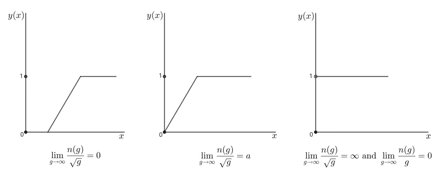
Define a function

y(x)\overset{\text{def}}{=}\liminf\limits_{g\to\infty}\textnormal{Prob}_{\textnormal{WP}}^{g}\left(X\in\mathcal{M}_{g,n(g)};\ \lambda_{1}(X)\leq x\right).

Then we may summarize Theorem 1, Theorem 2 and Theorem 3 as the following picture:

Refer to caption — Figure 1. Spectral gaps

Notations.

For any two non-negative functions $f$ and $h$ (may be of multi-variables), we say $h\succ f$ or $f\prec h$ if there exists a uniform constant $C>0$ such that $f\leq Ch$ . And we say $f\asymp h$ if $f\succ h$ and $f\prec h$ . For $0\leq m\leq n\in\mathbb{Z}$ , we use $\binom{n}{m}$ for binomial coefficient.

Plan of the paper.

Section 2 will provide a review of relevant background materials, and recall some useful results for Weil-Petersson measure, spectral theory, Cheeger constant and probability theory. In Section 3 we will firstly recall some results on Weil-Petersson volume of $\mathcal{M}_{g,n}$ , and then prove some estimations which will be applied later. In Section 4 we will introduce two special types of separating simple closed multi-curves and estimate the expected values of their related random variables. In Section 5 we will discuss three different types of $n(g)$ and finish the proofs of Theorem 1, 2 and 3. In Section 6 we will study Question 3 and give a partial answer to it.

Acknowledgement

We are grateful to the “Reading seminar on Teichmüller theory and related topics” at Tsinghua from which this work benefits a lot. We especially would like to thank Yuhao Xue for many helpful discussions on this project, and his comments on an earlier version, and thank Peter Zograf for his useful comments and informing us his early work [51] telling that for large enough $g$ , the set with $\lambda_{1}(X)<\epsilon$ in Theorem 1 is a full set provided that $\lim\limits_{g\to\infty}\frac{n(g)}{g}=\infty$ . We are also grateful to Zeev Rudnick for his interests, comments and suggestions on this work. The second named author is partially supported by NSFC grants No. 12171263, 12361141813, and 12425107.

2. Preliminaries

In this paper we use the same notations as in [36, 49]. In this section, we review the relevant background materials about Weil-Petersson metric, Mirzakhani’s Integration Formula, basic spectral theory for non-compact type hyperbolic surfaces, two elementary probabilistic results, Cheeger constant and so on.

2.1. Weil-Petersson symplectic form

Recall that for a surface $S_{g,n}$ of genus $g$ with $n$ punctures where $2g+n\geq 3$ , associated to a pants decomposition of $S_{g,n}$ , the Fenchel-Nielsen coordinate, given by $X\mapsto(\ell_{\alpha_{i}}(X),\tau_{\alpha_{i}}(X))_{i=1}^{3g+n-3},$ is a global coordinate for the Teichmüller space $\mathcal{T}_{g,n}$ of $S_{g,n}$ . Where $\{\alpha_{i}\}_{i=1}^{3g+n-3}$ are pairwisely disjoint simple closed curves, $\ell_{\alpha_{i}}(X)$ is the length of $\alpha_{i}$ on $X$ and $\tau_{\alpha_{i}}(X)$ is the twist along $\alpha_{i}$ (measured in length). Wolpert [46] showed that the Weil-Petersson symplectic structure has a magic form in Fenchel-Nielsen coordinates. More precisely,

Theorem 5 (Wolpert).

The Weil-Petersson symplectic form $\omega_{\mathrm{WP}}$ on $\mathcal{T}_{g,n}$ is given by

\omega_{\textnormal{WP}}=\sum_{i=1}^{3g+n-3}d\ell_{\alpha_{i}}\wedge d\tau_{\alpha_{i}}.

We mainly work with the Weil-Petersson volume form

d\mathit{vol}_{\mathrm{WP}}\overset{\text{def}}{=}\tfrac{1}{(3g+n-3)!}\underbrace{\omega_{\WP}\wedge\cdots\wedge\omega_{\WP}}_{\text{$3g+n-3$ copies}}~.

It is a mapping class group invariant measure on $\mathcal{T}_{g,n}$ , hence is the lift of a measure on the moduli space $\mathcal{M}_{g,n}$ of Riemann surfaces of genus $g$ with $n$ punctures, which we also denote by $d\mathit{vol}_{\WP}$ . The total volume of $\mathcal{M}_{g,n}$ is finite and we denote it by $V_{g,n}$ . The Weil-Petersson volume form is also well-defined on the weighted moduli space $\mathcal{M}_{g,n}(\boldsymbol{L})$ and its total volume, denoted by $V_{g,n}(\boldsymbol{L})$ , is finite.

Following Mirzakhani [32], we view a measurable function $f:\mathcal{M}_{g,n}\to\mathbb{R}$ as a random variable on $\mathcal{M}_{g,n}$ with respect to the probability measure $\textnormal{Prob}_{\textnormal{WP}}^{g,n}$ defined by normalizing $dvol_{\textnormal{WP}}$ , and let $\mathbb{E}_{\textnormal{WP}}^{g,n}[f]$ denote the expected value. Namely

\textnormal{Prob}_{\textnormal{WP}}^{g,n}(\mathcal{A})\overset{\text{def}}{=}\frac{1}{V_{g,n}}\int_{\mathcal{M}_{g,n}}\textbf{1}_{\mathcal{A}}dX,\ \mathbb{E}_{\textnormal{WP}}^{g,n}[f]\overset{\text{def}}{=}\frac{1}{V_{g,n}}\int_{\mathcal{M}_{g,n}}f(X)dX,

where $\mathcal{A}\subset\mathcal{M}_{g,n}$ is any Borel subset, $\mathbf{1}_{\mathcal{A}}:\mathcal{M}_{g,n}\to\{0,1\}$ is its characteristic function, and we always denote $dvol_{\mathrm{WP}}(X)$ as $dX$ for short. When $n=n(g)$ depends on $g$ , we write $\textnormal{Prob}_{\textnormal{WP}}^{g,n}$ and $\mathbb{E}_{\textnormal{WP}}^{g,n}$ as $\Prob$ and $\mathbb{E}_{\rm WP}^{g}$ for short respectively.

2.2. Mirzakhani’s Integration Formula

In this subsection we recall an integration formula due to Mirzakhani in [31, 32], which plays a role in the study of random surfaces in the Weil-Petersson model.

Given any non-peripheral closed curve $\gamma$ on a topological surface $S_{g,n}$ and a hyperbolic surface $X\in\mathcal{T}_{g,n}$ , we denote by $\ell_{\gamma}(X)$ the hyperbolic length of the unique closed geodesic representing $\gamma$ on $X$ . Let $\Gamma=(\gamma_{1},\cdots,\gamma_{k})$ be an ordered $k$ -tuple where the $\gamma_{i}$ ’s are distinct disjoint homotopy classes of nontrivial, non-peripheral, simple closed curves on $S_{g,n}$ . Let $\mathop{\rm Mod}_{g,n}$ be the mapping class group of $S_{g,n}$ . We consider the orbit containing $\Gamma$ under $\mathop{\rm Mod}_{g,n}$ action

\mathcal{O}_{\Gamma}=\{(h\cdot\gamma_{1},\cdots,h\cdot\gamma_{k});\ h\in\mathop{\rm Mod}\nolimits_{g,n}\}.

Given a function $F:\mathbb{R}^{k}_{\geq 0}\rightarrow\mathbb{R}_{\geq 0}$ , one may define a function on $\mathcal{M}_{g,n}$ as follows.

	$\displaystyle F^{\Gamma}:\mathcal{M}_{g,n}$	$\displaystyle\rightarrow$	$\displaystyle\mathbb{R}$
	$\displaystyle X$	$\displaystyle\mapsto$	$\displaystyle\sum_{(\alpha_{1},\cdots,\alpha_{k})\in\mathcal{O}_{\Gamma}}F(\ell_{\alpha_{1}}(X),\cdots,\ell_{\alpha_{k}}(X)).$

Assume $S_{g,n}\setminus\bigcup\limits_{j=1}^{k}\gamma_{j}\cong\bigcup\limits_{i=1}^{s}S_{g_{i},n_{i}}$ . We consider the volume

V_{g,n}(\Gamma,\boldsymbol{x})=\prod_{i=1}^{s}V_{g_{i},n_{i}}(\boldsymbol{x}^{(i)})

where $\boldsymbol{x}^{(i)}$ is the list of those coordinates $x_{j}$ of $\boldsymbol{x}$ such that $\gamma_{j}$ is a boundary component of $S_{g_{i},n_{i}}$ , and $V_{g_{i},n_{i}}(\boldsymbol{x}^{(i)})$ is the Weil-Petersson volume of the moduli space $\mathcal{M}_{g_{i},n_{i}}(\boldsymbol{x}^{(i)})$ . Mirzakhani established the following formula by applying Wolpert’s magic formula Theorem 5. One may also refer to [31, Theorem 7.1] or [33, Theorem 2.2] for more details on this formula.

Theorem 6 (Mirzakhani).

For any $\Gamma=(\gamma_{1},\cdots,\gamma_{k})$ , the integral of $F^{\Gamma}$ over $\mathcal{M}_{g,n}$ with respect to Weil-Petersson metric is given by

\int_{\mathcal{M}_{g,n}}F^{\Gamma}(X)dX=C_{\Gamma}\int_{\mathbb{R}^{k}_{\geq 0}}F(x_{1},\cdots,x_{k})V_{g,n}(\Gamma,\boldsymbol{x})\boldsymbol{x}\cdot d\boldsymbol{x}

where $\boldsymbol{x}\cdot d\boldsymbol{x}=x_{1}\cdots x_{k}dx_{1}\wedge\cdots\wedge dx_{k}$ and the constant $C_{\Gamma}\in(0,1]$ only depends on $\Gamma$ .

Remark.

Assume $\Gamma=(\gamma_{1},...,\gamma_{k})$ is a simple closed multi-curve on $S_{g,n}$ . If $(g,n)\neq(1,1),(2,0)$ , then the coffecient $C_{\Gamma}$ in Theorem 6 is given as

(1)

\displaystyle C_{\Gamma}=\frac{2^{-M(\Gamma)}}{|\textnormal{Stab}(\Gamma):\cap_{i=1}^{k}\textnormal{Stab}^{+}(\gamma_{i})|},

where

M(\Gamma)=|\{i;\ \gamma_{i}\text{ separates off a one-handle from }S_{g,n}\}|,

$\textnormal{Stab}(\Gamma)$ is the stablizer of $\Gamma$ and $\textnormal{Stab}^{+}(\gamma_{i})\ (1\leq i\leq k)$ is the subgroup of the mapping class group that fixes $\gamma_{i}$ and its orientation. For more details, one may refer to the footnote in [48, Page 368].

2.3. Basic spectral theory

For facts in this subsection, one may refer to e.g. [5, 7] for more details. Let $X\in\mathcal{M}_{g,n}$ where $n\geq 1$ be a non-compact hyperbolic surface of finite area, $\Delta$ be its Laplacian operator and $L^{2}(X)$ be the space of square-integrable functions on $X$ . Starting from the domain $\mathcal{D}\overset{\text{def}}{=}\{f\in C_{0}^{\infty}(X);\ \textit{$f$ and $\Delta f\in L^{2}(X)$}\}$ , the Friedrichs extension uniquely extends $\Delta$ to be a non-negative self-adjoint operator on $L^{2}(X)$ . The spectrum of $\Delta$ on $X$ consists of absolutely continuous spectrum $[\frac{1}{4},\infty)$ with multiplicity $n$ and possibly discrete spectrum in $[0,\infty)$ . A number $\lambda\geq 0$ is called an eigenvalue of $X$ if there exists a function $\phi\neq 0\in L^{2}(X)$ such that

\Delta\phi=\lambda\cdot\phi.

Clearly $0$ is an eigenvalue and the constant function $\frac{1}{\sqrt{\mathrm{Area(X)}}}$ is the normalized $0$ -eigenfunction. For a compact hyperbolic surface, its first non-zero eigenvalue can be determined by Rayleigh quotient through a Min-Max Principle. For non-compact hyperbolic surface, it is hard to detect the existence of a non-zero eigenvalue of $X$ (see Question 1). The following fundamental result for spectral theory is well-known and important for the existence of first eigenvalue in Theorem 1.

Theorem 7.

(see e.g. [40, Theorem XIII.1]) Let $X$ be a non-compact hyperbolic surface of finite area. If

\mathrm{RayQ}(X)\overset{\text{def}}{=}\inf\limits_{f\neq 0\in L^{2}(X);\int_{X}f=0}\frac{\int_{X}|\nabla f|^{2}}{\int_{X}f^{2}}<\frac{1}{4},

then $X$ has a non-zero first eigenvalue $\lambda_{1}(X)$ with $\lambda_{1}(X)=\mathrm{RayQ}(X)$ .

The second named author is grateful to Shiping Liu for pointing out the reference [40] to us. In this paper, we mainly study spectral gaps of Weil-Petersson random surfaces for large genus. For recent developments on spectral theory of Weil-Petersson random surfaces, one may see [15, 32, 35, 41] and references therein for related topics.

2.4. Probabilistic results

In this section, we recall two results from probability theory which will be applied later. For a probability space $(\Omega,\mathbb{P})$ , we have

Lemma 8.

For any non-negative integer-valued random variable $N$ , the following inequality holds:

\mathbb{P}(N\geq 1)\geq\frac{\mathbb{E}[N]^{2}}{\mathbb{E}[N^{2}]}

where $\mathbb{E}[\cdot]$ is the expected value.

Proof.

By Cauchy-Schwarz inequality, we have

	$\displaystyle\mathbb{E}[N]^{2}$	$\displaystyle=\mathbb{E}[N\cdot 1_{\{N\geq 1\}}]^{2}$
		$\displaystyle\leq\mathbb{E}[N^{2}]\cdot\mathbb{E}[1^{2}_{\{N\geq 1\}}]$
		$\displaystyle=\mathbb{E}[N^{2}]\cdot\mathbb{P}(N\geq 1).$

It follows that

\mathbb{P}(N\geq 1)\geq\frac{\mathbb{E}[N]^{2}}{\mathbb{E}[N^{2}]}

as desired. ∎

Let $\mathbb{N}$ be the set of all positive integers. For any $r\in\mathbb{N}$ and a random variable $N:\Omega\to\mathbb{N}\cup\{0\}$ , we define the random variable

(N)_{r}\overset{\text{def}}{=}N(N-1)\cdots(N-r+1).

If the expected value $\mathbb{E}[(N)_{r}]$ of $(N)_{r}$ exists, then it is called the $r$ -th factorial moment of $N$ . Recall that a non-negative integer-valued random variable $N$ is said to be Poisson distributed with mean $\lambda\in[0,\infty)$ if

\mathbb{P}(N=k)=\frac{\lambda^{k}e^{-\lambda}}{k!}\text{ for all }k\in\mathbb{N}\cup\{0\}.

It is known that a non-negative integer-valued random variable $N$ is Poisson distributed if and only if its $r$ -th factorial moment is equal to $\lambda^{n}$ for all $r\in\mathbb{N}$ . This can be generalized to the following form (see e.g. [33, Theorem 2.9] or [6, Theorem 1.21]):

Theorem 9.

Let $\{N_{n}\}_{n\geq 1}$ be a sequence of non-negative integer-valued random variables. If there exists a constant $\lambda>0$ such that for all $r\in\mathbb{N}$ ,

\lim\limits_{n\to\infty}\mathbb{E}\left[(N_{n})_{r}\right]=\lambda^{r},

then we have for all $k\in\mathbb{N}\cup\{0\}$ ,

\lim\limits_{n\to\infty}\mathbb{P}(N_{n}=k)=\frac{\lambda^{k}e^{-\lambda}}{k!}.

2.5. Cheeger constant

For any hyperbolic surface $X$ , the Cheeger constant $h(X)$ of $X$ is defined as

h(X)\overset{\text{def}}{=}\inf\limits_{E\subset X}\frac{\ell(E)}{\min\{\textnormal{Area}(X_{1}),\textnormal{Area}(X_{2})\}}

where $E$ runs over all rectifiable one-dimensional subsets of $X$ which divide $X$ into two disjoint components $X_{1}$ and $X_{2}$ , $\ell(E)$ is the length of $E$ , and $\textnormal{Area}(X_{i})$ is the area of $X_{i}$ for $i=1,2$ . For the case that $X$ is compact, let $\lambda_{1}(X)$ be the first eigenvalue of the Laplacian operator on $X$ , the Cheeger’s inequality [11] tells that

\lambda_{1}(X)\geq\frac{1}{4}h^{2}(X).

For the case that $X$ is non-compact, since the existence of the first eigenvalue is not clear, we consider $\textnormal{RayQ}(X)$ instead of $\lambda_{1}(X)$ . The following Cheeger’s inequality for cusped hyperbolic surfaces will be applied in the proof of Theorem 3.

Lemma 10 (see e.g. [9, Page 228]).

Assume $X$ is a complete hyperbolic surface of finite area, then

\textnormal{RayQ}(X)\geq\frac{1}{4}h^{2}(X).

For inverse Cheeger’s inequality, Buser proved that

Theorem 11 ([9, Theorem 7.1]).

If $X$ is a complete, non-compact hyperbolic surface, then

\textnormal{RayQ}(X)\leq c\cdot h(X)

where $c>0$ is a universal constant.

2.6. Geodesic Cheeger constant

Adams and Morgan investigated the isoperimetric problem on hyperbolic surfaces in [1]. The following result is about the characterization of perimeter minimizers for cusped hyperbolic surfaces.

Theorem 12 ([1, Theorem 2.2]).

Let $X$ be a complete non-compact hyperbolic surface of finite area. For given area $0<A<\textnormal{area}(X)$ , a perimeter-minimizing system of embedded rectifiable curves bounding a region $R$ of area $A$ consists of a set of curves of one of the following types:

(1)

horocycles around cusps;
(2)

geodesics or single “neighboring curves” at constant distance from a geodesic.

The total perimeter $L(A)$ of a minimizer of area $A$ satisfies that $L(A)\leq A$ , and if $A<\pi$ , then a minimizer consists of neighborhoods of an arbitrary collection of cusps bounded by horocycles, of total length $A$ .

From Theorem 12, we have

h(X)=\inf\limits_{0<A\leq\frac{\textnormal{Area}(X)}{2}}\frac{L(A)}{A},

and

L(A)=A\text{ for all }0<A<\pi.

Hence the infimum above is realized at some value in $\left[\frac{\pi}{2},\frac{\textnormal{Area}(X)}{2}\right]$ . Denote by

\mathcal{S}(X)=\left(\alpha=\bigcup\limits_{i=1}^{k}\alpha_{i};\ \begin{matrix}\text{For all }1\leq i\leq k,\ \alpha_{i}\text{ is a simple closed curve in $X$, }\\ \text{and }X\setminus\alpha=X_{1}\cup X_{2},\text{ where $X_{1}$ and $X_{2}$ are}\\ \text{two disjoint connected components.}\end{matrix}\right)

and

\mathcal{SG}(X)=\left(\alpha=\bigsqcup\limits_{i=1}^{k}\alpha_{i};\ \begin{matrix}\text{For all }1\leq i\leq k,\ \alpha_{i}\text{ is a simple closed geodesic in $X$, }\\ \text{and }X\setminus\alpha=X_{1}\cup X_{2},\text{ where $X_{1}$ and $X_{2}$ are}\\ \text{two disjoint connected components.}\end{matrix}\right).

For any $\alpha\in\mathcal{S}(X)$ such that $X\setminus\alpha=X_{1}\cup X_{2}$ , denote by

(2)

\mathcal{H}(\alpha)=\frac{\ell(\alpha)}{\min\{\textnormal{Area}(X_{1}),\textnormal{Area}(X_{2})\}}

where $\ell(\alpha)$ is the hyperbolic length of $\alpha$ and $\textnormal{Area}(X_{i})$ is the area of $X_{i}$ for $i=1,2$ . Due to S. T. Yau (see e.g. [10, Theorem 8.3.6]) and Theorem 12, one may check that

(3)

\displaystyle h(X)=\inf\limits_{\alpha\in\mathcal{S}(X)}\mathcal{H}(\alpha).

Mirzakhani defined the geodesic Cheeger constant in [32] as

H(X)\overset{\textnormal{def}}{=}\min\limits_{\alpha\in\mathcal{SG}(X)}\mathcal{H}(\alpha).

Based on Theorem 12, Mirzakhani [32] observed the following connection between $H(X)$ and $h(X)$ . Assume $\alpha=\bigcup_{i=1}^{k}\alpha_{i}\in\mathcal{S}(X)$ and $\alpha^{\prime}=\bigcup_{i=1}^{k}\alpha_{i}^{\prime}\in\mathcal{SG}(X)$ such that $\alpha_{i}$ is a neighboring curve at a constant distance from a simple closed geodesic $\alpha_{i}^{\prime}$ for all $1\leq i\leq k$ . Then a simple computation yields that

(4)

\displaystyle\mathcal{H}(\alpha)\geq\frac{\mathcal{H}(\alpha^{\prime})}{1+\mathcal{H}(\alpha^{\prime})}.

This implies that

Proposition 13 ([32, Proposition 4.7]).

Let $X$ be a complete non-compact hyperbolic surface of finite area, then

\frac{H(X)}{1+H(X)}\leq h(X)\leq H(X).

Remark.

Mirzakhani stated [32, Proposition 4.7] only for closed hyperbolic surfaces. Actually its proof also leads to the case of cusped hyperbolic surfaces.

3. WP volume

In this section, we first recall several estimates about the Weil-Petersson volume $V_{g,n}$ of moduli space $\mathcal{M}_{g,n}$ . Then we provide certain useful bounds on $V_{g,n}$ which will be applied in the proofs of Theorem 1, 2 and 3.

3.1. Asymptotic properties on $V_{g,n}$

In this subsection, we first recall several results about $V_{g,n}$ , and then make two useful estimations. One may also see [37, 44, 31, 32, 34, 3, 2] and references therein for the asymptotic behavior of $V_{g,n}$ and its deep connection to the intersection theory of $\mathcal{M}_{g,n}$ .

We always let $V_{0,3}(x,y,z)=1$ (see [31, Table $1$ ]). The following lemma is due to Mirzakhani.

Lemma 14 ([32, Lemma 3.2]).

For any $g,n\geq 0$ with $2g-2+n>0$ , we have

(1)

$V_{g,n}\leq V_{g,n}(x_{1},\cdots,x_{n})\leq e^{\frac{x_{1}+\cdots+x_{n}}{2}}V_{g,n},$
(2)

$V_{g-1,n+4}\leq V_{g,n+2}$

and

$\frac{V_{g,n+1}}{(2g-2+n)V_{g,n}}\asymp 1.$

The following two results are due to Mirzakhani-Zograf.

Lemma 15 ([34, Lemma 5.1]).

There exists a universal constant $c_{2}>0$ such that for any $g,n\geq 0$ with $2g-2+n\geq 1$ , the following inequality holds:

\left|\frac{(2g-2+n)V_{g,n}}{V_{g,n+1}}-\frac{1}{4\pi^{2}}\right|\leq\frac{c_{2}n}{2g-2+n}.

As a direct consequence, we have

Lemma 16.

If $n(g)$ satisfies that $\lim\limits_{g\to\infty}\frac{n(g)}{g}=0,$ then we have

\lim\limits_{g\to\infty}\frac{V_{g,n(g)}^{2}}{V_{g,n(g)-1}V_{g,n(g)+1}}=1.

Mirzakhani and Zograf also proved the following aysmptotic behavior of $V_{g,n}$ for large $g$ .

Theorem 17 ([34, Theorem 1.2]).

There exists a universal constant $C>0$ such that for any given $n\geq 0$ ,

V_{g,n}=\frac{C}{\sqrt{g}}(2g-3+n)!\cdot(4\pi^{2})^{2g-3+n}\cdot\left(1+O\left(\frac{1}{g}\right)\right)

as $g\rightarrow\infty$ . The implied constant is related to $n$ and independent of $g$ .

Remark.

It is conjectured by Zograf in [50] that $C=\frac{1}{\sqrt{\pi}}$ .

Now we apply the results above to get several useful new bounds on $V_{g,n}$ . Our first one is as follows.

Lemma 18.

For any non-negative integers $g,n$ such that $2g-2+n\geq 2$ ,

V_{g,n}\prec\frac{(2g-3+n)!\cdot(4\pi^{2})^{2g-3+n}}{\sqrt{2g-2+n}}.

Proof.

From Part $(2)$ of Lemma 14 and the assumption that $2g-2+n\geq 2$ , there exist $g^{\prime}>0$ and $0\leq n^{\prime}\leq 3$ such that

2g-2+n=2g^{\prime}-2+n^{\prime}\text{ and }V_{g,n}\leq V_{g^{\prime},n^{\prime}}.

Apply Theorem 17 to $V_{g^{\prime},n^{\prime}}$ , we have

	$\displaystyle V_{g,n}$	$\displaystyle\leq V_{g^{\prime},n^{\prime}}\prec\frac{(2g^{\prime}-3+n^{\prime})!\cdot(4\pi^{2})^{2g^{\prime}-3+n^{\prime}}}{\sqrt{g^{\prime}}}$
		$\displaystyle\prec\frac{(2g-3+n)!\cdot(4\pi^{2})^{2g-3+n}}{\sqrt{2g-2+n}}$

where the last inequality holds since $2g-2+n\prec g^{\prime}$ . The proof is complete. ∎

The following lemma is implicitly contained in the proof of [34, Theorem 1.8]. We prove it here for completeness.

Lemma 19.

Assume $n(g)\prec\sqrt{g}$ , then we have

V_{g,n(g)}\asymp\frac{(2g-3+n(g))!\cdot(4\pi^{2})^{2g-3+n(g)}}{\sqrt{g}}.

Proof.

It suffices to consider the case when $g$ is large. From Lemma 15, there exists a universal constant $c_{3}>0$ such that for any $0\leq n\leq n(g)$ and large enough $g$ ,

(5)

\displaystyle\frac{1}{4\pi^{2}}\left(1-\frac{c_{3}n}{g}\right)\leq\frac{(2g-2+n)V_{g,n}}{V_{g,n+1}}\leq\frac{1}{4\pi^{2}}\left(1+\frac{c_{3}n}{g}\right).

Denote by

\mu_{1}=\prod\limits_{i=1}^{n(g)}\left(1-\frac{c_{3}i}{g}\right)\text{ and }\mu_{2}=\prod\limits_{i=1}^{n(g)}\left(1+\frac{c_{3}i}{g}\right).

It is clear that for $x>0$ small enough, $\log(1+x)\leq x$ and $\log(1-x)\geq-2x$ . Since $n(g)\prec\sqrt{g}$ , it follows that for $g$ large enough,

\log\mu_{1}=\sum\limits_{i=1}^{n(g)}\log\left(1-\frac{c_{3}i}{g}\right)\geq\sum\limits_{i=1}^{n(g)}-\frac{2c_{3}i}{g}\asymp-\frac{n(g)^{2}}{g}\succ-1

and

\displaystyle\log\mu_{2}=\sum\limits_{i=1}^{n(g)}\log\left(1+\frac{c_{3}i}{g}\right)\leq\sum\limits_{i=1}^{n(g)}\frac{c_{3}i}{g}\asymp\frac{n(g)^{2}}{g}\prec 1.

Hence one may assume that there exists a universal constant $c_{4}>1$ such that

(6)

\displaystyle\frac{1}{c_{4}}<\mu_{1}<\mu_{2}<c_{4}.

For any $g,n\geq 0$ with $2g-2+n\geq 2$ , denote by

C_{g,n}=\frac{(2g-3+n)!\cdot(4\pi^{2})^{2g-3+n}}{\sqrt{g}}.

Then we have

\frac{V_{g,n(g)}}{C_{g,n(g)}}=\prod\limits_{i=0}^{n(g)-1}\frac{V_{g,n(g)-i}}{4\pi^{2}(2g-3+n(g)-i)V_{g,n(g)-i-1}}\cdot\frac{V_{g,0}}{C_{g,0}}.

Together with (5) and (6), it follows that

\frac{1}{c_{4}}\cdot\frac{V_{g,0}}{C_{g,0}}\leq\frac{1}{\mu_{2}}\cdot\frac{V_{g,0}}{C_{g,0}}\leq\frac{V_{g,n(g)}}{C_{g,n(g)}}\leq\frac{1}{\mu_{1}}\cdot\frac{V_{g,0}}{C_{g,0}}\leq c_{4}\cdot\frac{V_{g,0}}{C_{g,0}}.

Then the proof is complete by applying Theorem 17. ∎

3.2. A useful bound for WP volume

For $m\in\mathbb{N}$ and non-negative integers $g,n(g)$ with

(7)

\chi\overset{\text{def}}{=}2g-2+n(g)\geq 1,

we denote by $\mathcal{I}_{m}$ the set consisting of all 4-tuples of non-negative integers $(g_{1},n_{1},g_{2},n_{2})$ satisfying the following conditions:

(a)

$2g_{1}-2+n_{1}+2g_{2}-2+n_{2}=\chi$ .
(b)

$m=2g_{1}-2+n_{1}\leq 2g_{2}-2+n_{2}$ .
(c)

$n(g)-n_{1}\leq n_{2}\leq n(g)+n_{1}$ , $n_{1},n_{2}\geq 1$ .

From condition $(b)$ , there are at most $m+2$ different choices for $(g_{1},n_{1})$ . Since $n_{1}\leq m+2$ , together with condition $(c)$ , there are at most $2m+5$ different choices for $n_{2}$ . Recall that from condition $(b)$ , $g_{1}$ is uniquely determined by $n_{1}$ and $m$ . Thus it follows that

(8)

\displaystyle\left|\mathcal{I}_{m}\right|\leq 2(m+3)^{2}.

Lemma 20.

Assume $n(g)\prec\sqrt{g}$ . Then for any pair $(g_{1},n_{1},g_{2},n_{2})\in\mathcal{I}_{m}$ ,

\frac{V_{g_{1},n_{1}}V_{g_{2},n_{2}}}{V_{g,n(g)}}\prec\frac{m^{m}(\chi-m)^{\chi-m}}{\chi^{\chi}}.

Proof.

Since $2m\leq\chi$ and $n(g)\prec\sqrt{g}$ ,

(9)

(\chi-m)\asymp\chi\asymp g.

Then by Lemma 19 we have

(10)

V_{g,n(g)}\asymp\frac{(\chi-1)!\cdot(4\pi^{2})^{\chi}}{\sqrt{\chi}}.

By Lemma 18 we also have

(11)

V_{g_{1},n_{1}}\prec\frac{(m-1)!\cdot(4\pi^{2})^{m}}{\sqrt{m}}\textit{\ and \ }V_{g_{2},n_{2}}\prec\frac{(\chi-m-1)!\cdot(4\pi^{2})^{\chi-m}}{\sqrt{\chi-m}}.

Combining (9), (10) and (11), we have

(12)

\frac{V_{g_{1},n_{1}}V_{g_{2},n_{2}}}{V_{g,n(g)}}\prec\frac{(m-1)!(\chi-m-1)!}{(\chi-1)!}\cdot\frac{\sqrt{g}}{\sqrt{m}\sqrt{\chi-m}}\prec\frac{m!(\chi-m)!}{\chi!}\cdot\frac{1}{m}.

Recall that the Stirling’s formula says that

k!\sim\sqrt{2\pi k}\left(\frac{k}{e}\right)^{k}.

Plug it into (12), we get

\frac{V_{g_{1},n_{1}}V_{g_{2},n_{2}}}{V_{g,n(g)}}\prec\frac{m^{m}(\chi-m)^{\chi-m}}{\chi^{\chi}}\cdot\frac{\sqrt{\chi-m}}{\sqrt{m}\sqrt{\chi}}\prec\frac{m^{m}(\chi-m)^{\chi-m}}{\chi^{\chi}}

as desired. ∎

Now we prove the following result which is useful in the proof of Theorem 3.

Proposition 21.

Assume $n(g)\prec\sqrt{g}$ . For $0<u<\frac{\log 2}{2\pi}$ and $m\geq 2\in\mathbb{N}$ , set

L_{m}=2\pi mu+3\cdot(2\pi mu)^{\frac{2}{3}}.

Then we have

\frac{1}{V_{g,n(g)}}\sum\limits_{m=2}^{\lfloor\frac{\chi}{2}\rfloor}\sum\limits_{(g_{1},n_{1},g_{2},n_{2})\in\mathcal{I}_{m}}C(m,n(g))V_{g_{1},n_{1}}V_{g_{2},n_{2}}e^{L_{m}}\prec\frac{1}{\sqrt{g}},

where $C(m,n(g))=\max\limits_{0\leq i\leq m+1}\binom{n(g)}{i}.$

Proof.

Since $n(g)\prec\sqrt{g}$ , one may assume $n(g)\leq a\sqrt{g}$ for some $a>0$ . It suffices to consider for large enough $g$ . For all $2\leq m\leq\lfloor\frac{\chi}{2}\rfloor$ , set

A_{m}=\frac{1}{V_{g,n(g)}}\sum\limits_{(g_{1},n_{1},g_{2},n_{2})\in\mathcal{I}_{m}}C(m,n(g))V_{g_{1},n_{1}}V_{g_{2},n_{2}}e^{L_{m}}.

Since $u<\frac{\log 2}{2\pi}$ , it follows that for $m$ large enough

\displaystyle e^{\frac{L_{m}}{m}}=e^{2\pi u+3(2\pi u)^{\frac{2}{3}}m^{-\frac{1}{3}}}<2-\delta

for some constant $\delta>0$ only depending on $u$ . So we have for all $m\geq 2$ ,

\displaystyle e^{L_{m}}\prec(2-\delta)^{m}.

Then from (8) and Lemma 20 we have

(13)		$\displaystyle A_{m}$	$\displaystyle\prec C(m,n(g))\frac{m^{m}(\chi-m)^{\chi-m}}{\chi^{\chi}}e^{L_{m}}m^{2}$
		$\displaystyle\prec C(m,n(g))\left(\frac{m(2-\delta)}{\chi}\right)^{m}m^{2}.$

It is clear that for any $m\geq 2$ , we also have

(14)

\displaystyle\max\limits_{0\leq i\leq m+1}\binom{n(g)}{i}=\max\limits_{0\leq i\leq m+1}\frac{n(g)!}{i!\cdot(n(g)-i)!}\leq\min\left\{n(g)^{m+1},2^{n(g)}\right\}.

Next we split the argument into four different cases.

Case I: $g^{\frac{3}{4}}\leq m\leq\lfloor\frac{\chi}{2}\rfloor$ . From (13) and (14) we have

	$\displaystyle A_{m}$	$\displaystyle\prec C(m,n(g))\left(\frac{m(2-\delta)}{\chi}\right)^{m}m^{2}$
		$\displaystyle\prec 2^{\left\lfloor a\sqrt{g}\right\rfloor}\left(\frac{2-\delta}{2}\right)^{\left\lfloor g^{\frac{3}{4}}\right\rfloor}g^{2}\prec\frac{1}{g^{2}}.$

Then it follows that

(15)

\displaystyle\sum\limits_{m=\left\lfloor g^{\frac{3}{4}}\right\rfloor+1}^{\lfloor\frac{\chi}{2}\rfloor}A_{m}\prec\frac{1}{g}.

Case II: $\frac{\sqrt{g}}{4ea}\leq m\leq g^{\frac{3}{4}}$ . From (13) and (14) we have

	$\displaystyle A_{m}$	$\displaystyle\prec C(m,n(g))\left(\frac{m(2-\delta)}{\chi}\right)^{m}m^{2}$
		$\displaystyle\prec 2^{\left\lfloor a\sqrt{g}\right\rfloor}\left(\frac{2}{g^{\frac{1}{4}}}\right)^{\left\lfloor\frac{\sqrt{g}}{4ea}\right\rfloor}m^{2}$
		$\displaystyle\prec\left(\frac{2^{4ea^{2}+1}}{g^{\frac{1}{4}}}\right)^{\left\lfloor\frac{\sqrt{g}}{4ea}\right\rfloor}\cdot g^{3}\prec\frac{1}{g^{2}}.$

Then it follows that

(16)

\displaystyle\sum\limits_{m=\lfloor\frac{\sqrt{g}}{4ea}\rfloor}^{\lfloor g^{\frac{3}{4}}\rfloor}A_{m}\prec\frac{1}{g}.

Case III: $4\log g\leq m\leq\frac{\sqrt{g}}{4ea}$ . For this case we have $n(g)\cdot m\leq a\sqrt{g}\cdot\frac{\sqrt{g}}{4ea}=\frac{g}{4e}$ . Then from (13) and (14) we have

	$\displaystyle A_{m}$	$\displaystyle\prec n(g)^{m+1}\left(\frac{m(2-\delta)}{\chi}\right)^{m}m^{2}$
		$\displaystyle\prec\left(\frac{2n(g)m}{\chi}\right)^{m}n(g)m^{2}$
		$\displaystyle\prec\left(\frac{1}{e}\right)^{m}n(g)\cdot g\prec\left(\frac{1}{e}\right)^{m}g^{\frac{3}{2}}.$

Then it follows that

(17)

\displaystyle\sum\limits_{m=\left\lfloor 4\log g\right\rfloor}^{\left\lfloor\frac{\sqrt{g}}{4ea}\right\rfloor}A_{m}\prec\sum\limits_{m=\left\lfloor 4\log g\right\rfloor}^{\left\lfloor\frac{\sqrt{g}}{4ea}\right\rfloor}\left(\frac{1}{e}\right)^{m}g^{\frac{3}{2}}\prec e^{-4\log g}\cdot\sqrt{g}\cdot g^{\frac{3}{2}}\prec\frac{1}{g}.

Case IV: $2\leq m\leq 4\log g$ . From (13) and (14) we have

(18)	$\displaystyle\sum\limits_{m=2}^{\left\lfloor 4\log g\right\rfloor}A_{m}$	$\displaystyle\prec\sum\limits_{m=2}^{\left\lfloor 4\log g\right\rfloor}n(g)^{m+1}\left(\frac{m(2-\delta)}{\chi}\right)^{m}m^{2}$
	$\displaystyle\prec\sum\limits_{m=2}^{\left\lfloor 4\log g\right\rfloor}\left(\frac{2am}{\sqrt{g}}\right)^{m}n(g)m^{2}$
	$\displaystyle\leq\frac{64a^{2}n(g)}{g}+\sum\limits_{m=3}^{\left\lfloor 4\log g\right\rfloor}\left(\frac{8a\log g}{\sqrt{g}}\right)^{3}n(g)(4\log g)^{2}\prec\frac{1}{\sqrt{g}}.$

Then the conclusion follows from (15), (16), (17) and (18). ∎

3.3. Intersection number and WP volume

Recall that on $\overline{\mathcal{M}}_{g,n}$ the compactified moduli space of surfaces of genus $g$ with $n$ punctures, there are $n$ tautological line bundles $\{\mathcal{L}_{i}\}_{i=1}^{n}$ . Let $\psi_{i}=c_{1}(\mathcal{L}_{i})\in H_{2}(\overline{\mathcal{M}}_{g,n},\mathbb{Q})$ be the first Chern class of $\mathcal{L}_{i}$ and $\omega$ be the Weil-Petersson symplectic form on $\overline{\mathcal{M}}_{g,n}$ . For any $\textbf{d}=(d_{1},\cdots,d_{n})$ with each $d_{i}\in\mathbb{Z}_{\geq 0}$ and $|\textbf{d}|=d_{1}+\cdots+d_{n}\leq 3g-3+n$ , the intersection number $\left[\tau_{d_{1}}\cdots\tau_{d_{n}}\right]_{g,n}$ is defined as

\left[\tau_{d_{1}}\cdots\tau_{d_{n}}\right]_{g,n}=\left[\prod\limits_{i=1}^{n}\tau_{d_{i}}\right]_{g,n}\overset{\text{def}}{=}\frac{\prod_{i=1}^{n}2^{2d_{i}}(2d_{i}+1)!!}{(3g-3+n-|d|)!}\int_{\overline{\mathcal{M}}_{g,n}}\psi_{1}^{d_{1}}\cdots\psi_{n}^{d_{n}}\omega^{3g-3+n-|d|}.

In particular, $\left[\tau_{0}\cdots\tau_{0}\right]_{g,n}=\mathop{\rm Vol}(\mathcal{M}_{g,n})$ , which is also denoted by $V_{g,n}$ .

In this subsection we use the same notations as in [32, 34]. Recall [32, (3.1)] tells that for $x_{i}\geq 0\ (1\leq i\leq n)$

(19)

\displaystyle V_{g,n}(2x_{1},...,2x_{n})=\sum\limits_{|\textbf{d}|\leq 3g-3+n}\left[\prod\limits_{i=1}^{n}\tau_{d_{i}}\right]_{g,n}\cdot\prod\limits_{i=1}^{n}\frac{x_{i}^{2d_{i}}}{(2d_{i}+1)!}.

To bound $V_{g,n}(2x_{1},...,2x_{n})$ , it suffices to bound the intersection numbers $\left[\prod\limits_{i=1}^{n}\tau_{d_{i}}\right]_{g,n}$ .

As in [32] we let $a_{0}=\frac{1}{2}$ and for $i\geq 1$ ,

a_{i}=\zeta(2i)(1-2^{1-2i}),

where $\zeta(\cdot)$ is the Riemann zeta function.

Lemma 22 ([34, Lemma 2.2]).

The sequence $\{a_{i}\}_{i=0}^{\infty}$ is increasing. Moreover,

(1)

$\lim\limits_{i\to\infty}a_{i}=1.$
(2)

There exists $C>1$ such that

$\frac{1}{C\cdot 2^{2i}}<a_{i+1}-a_{i}<\frac{C}{2^{2i}}.$

As a direct consequence, for any $k\in\mathbb{N}$ ,

(20)

\displaystyle\sum\limits_{L=1}^{\infty}(L+k)(a_{L+k}-a_{L})\prec k.

For any $\textbf{d}=(d_{1},\cdots,d_{n})$ , let $d_{0}=3g-3+n-|\textbf{d}|$ , the Recursive Formula (see [32, Section 3.1]) says that

\left[\prod\limits_{i=1}^{n}\tau_{d_{i}}\right]_{g,n}=\left(\sum\limits_{j=2}^{n}\mathcal{A}_{\textbf{d}}^{j}\right)+\mathcal{B}_{\textbf{d}}+\mathcal{C}_{\textbf{d}},

where

\mathcal{A}_{\textbf{d}}^{j}=8\sum\limits_{L=0}^{d_{0}}(2d_{j}+1)a_{L}\left[\tau_{d_{1}+d_{j}+L-1}\cdot\prod\limits_{i\neq 1,j}\tau_{d_{i}}\right]_{g,n-1},

\mathcal{B}_{\textbf{d}}=16\sum\limits_{L=0}^{d_{0}}\sum\limits_{k_{1}+k_{2}=L+d_{1}-2}a_{L}\left[\tau_{k_{1}}\tau_{k_{2}}\prod\limits_{i\neq 1}\tau_{d_{i}}\right]_{g,n+1},

and

	$\displaystyle\mathcal{C}_{\textbf{d}}$	$\displaystyle=16\sum\limits_{\begin{subarray}{c}I\sqcup J=\{2,...,n\}\\ 0\leq g^{\prime}\leq g\end{subarray}}\sum\limits_{L=0}^{d_{0}}\sum\limits_{k_{1}+k_{2}=L+d_{1}-2}a_{L}\left[\tau_{k_{1}}\prod\limits_{i\in I}\tau_{d_{i}}\right]_{g^{\prime},\|I\|+1}$
		$\displaystyle\times\left[\tau_{k_{2}}\prod\limits_{i\in J}\tau_{d_{i}}\right]_{g-g^{\prime},\|J\|+1}.$

Through comparing the coefficients of $\mathcal{A}_{\textbf{d}},\mathcal{B}_{\textbf{d}}$ and $\mathcal{C}_{\textbf{d}}$ , it is not hard to see that (see [34, Equation 3.6])

(21)

\displaystyle\left[\prod\limits_{i=1}^{n}\tau_{d_{i}}\right]_{g,n}\leq V_{g,n}.

Now we prove the following result.

Lemma 23.

Assume $n\prec\sqrt{g}$ , and set $\textbf{d}=(d_{1},...,d_{n})$ and $\textbf{d}^{\prime}=(d_{1}^{\prime},...,d_{n}^{\prime})=(0,d_{2},...,d_{n})$ . Then there exists a constant $C>0$ such that

0\leq\left[\prod\limits_{i=1}^{n}\tau_{d_{i}^{\prime}}\right]_{g,n}-\left[\prod\limits_{i=1}^{n}\tau_{d_{i}}\right]_{g,n}\leq\frac{C|\textbf{d}|(|\textbf{d}|+n)}{g}\cdot V_{g,n}.

Proof.

Since the proof is similar to the proofs of [32, Equation 3.23] and [34, Lemma 5.1], we only give an outline here. For the LHS inequality, it directly follows by comparing the terms $\mathcal{A}_{\textbf{d}}^{j}$ , $\mathcal{B}_{\textbf{d}}^{j}$ and $\mathcal{C}_{\textbf{d}}^{j}$ with $\mathcal{A}_{\textbf{d}^{\prime}}^{j}$ , $\mathcal{B}_{\textbf{d}^{\prime}}^{j}$ and $\mathcal{C}_{\textbf{d}^{\prime}}^{j}$ respectively in the Recursive Formula above. For the RHS inequality, $\mathrm{WLOG}$ one may first assume that $d_{1}>0$ . Then compare the terms $\mathcal{A},\mathcal{B}$ and $\mathcal{C}$ respectively, it follows from Lemma 22 and (21) that for any fixed $2\leq j\leq n$ ,

		$\displaystyle\ \ \ \ \mathcal{A}_{\textbf{d}^{\prime}}^{j}-\mathcal{A}_{\textbf{d}}^{j}$
		$\displaystyle=8\sum\limits_{L=0}^{d_{0}}(2d_{j}+1)a_{L}\left[\tau_{d_{j}+L-1}\cdot\prod\limits_{i\neq 1,j}\tau_{d_{i}}\right]_{g,n-1}$
		$\displaystyle-8\sum\limits_{L=0}^{d_{0}}(2d_{j}+1)a_{L}\left[\tau_{d_{1}+d_{j}+L-1}\cdot\prod\limits_{i\neq 1,j}\tau_{d_{i}}\right]_{g,n-1}$
		$\displaystyle=8(2d_{j}+1)\sum\limits_{t=d_{j}-1}^{d_{0}+d_{j}-1}a_{t-(d_{j}-1)}\left[\tau_{t}\prod\limits_{i\neq 1,j}\tau_{d_{i}}\right]_{g,n-1}$
		$\displaystyle-8(2d_{j}+1)\sum\limits_{t=d_{1}+d_{j}-1}^{d_{0}+d_{1}+d_{j}-1}a_{t-(d_{1}+d_{j}-1)}\left[\tau_{t}\prod\limits_{i\neq 1,j}\tau_{d_{i}}\right]_{g,n-1}$
		$\displaystyle\leq 8d_{1}(2d_{j}+1)V_{g,n-1}+\sum\limits_{t=d_{1}+d_{j}-1}^{d_{0}+d_{j}-1}(a_{t-(d_{j}-1)}-a_{t-(d_{1}+d_{j}-1)})V_{g,n-1}$
		$\displaystyle\prec\frac{d_{1}(2d_{j}+1)}{g}\cdot V_{g,n}\prec\frac{\max_{1\leq i\leq n}d_{i}\cdot(2d_{j}+1)}{g}\cdot V_{g,n}.$

This leads to

\sum\limits_{j=2}^{n}(\mathcal{A}_{\textbf{d}^{\prime}}^{j}-\mathcal{A}_{\textbf{d}}^{j})\prec\frac{\max_{1\leq i\leq n}d_{i}\cdot(|\textbf{d}|+n)}{g}\cdot V_{g,n}\prec\frac{|\textbf{d}|(|\textbf{d}|+n)}{g}\cdot V_{g,n}.

Similarly, by applying (20) and (21), we have

\displaystyle\mathcal{B}_{\textbf{d}^{\prime}}-\mathcal{B}_{\textbf{d}}\prec\frac{|\textbf{d}|^{2}}{g}\cdot V_{g,n}.

For the term $\mathcal{C}$ , first by Lemma 18 and 19 it is not hard to see that

\sum\limits_{(g_{1},n_{1},g_{2},n_{2})}\binom{n-1}{n_{1}}\cdot\frac{V_{g_{1},n_{1}+1}V_{g_{2},n_{2}+1}}{V_{g,n}}=O\left(\frac{n^{2}}{g^{2}}\right)

where $(g_{1},n_{1},g_{2},n_{2})$ runs over all pairs of non-negative integers such that

g_{1}+g_{2}=g\text{ and }n_{1}+n_{2}=n-1.

Then similar as the proof for $\mathcal{A}_{\textbf{d}^{\prime}}^{j}-\mathcal{A}_{\textbf{d}}^{j}$ , by applying (20) and (21) one may have

\mathcal{C}_{\textbf{d}^{\prime}}-\mathcal{C}_{\textbf{d}}\prec\frac{n^{2}|\textbf{d}|^{2}}{g^{2}}\cdot V_{g,n}\prec\frac{|\textbf{d}|^{2}}{g}\cdot V_{g,n}.

Then the conclusion follows by taking a summation over all $\mathcal{A}_{\textbf{d}}^{j},\ \mathcal{B}_{\textbf{d}}$ and $\mathcal{C}_{\textbf{d}}$ . ∎

Lemma 24.

Assume $n(g)\prec\sqrt{g}$ and $k\in\mathbb{N}$ , then there exists a constant $C>0$ such that for any $\textbf{d}=(d_{1},...,d_{k})$ with $d_{i}\geq 0$ and $|\textbf{d}|=d_{1}+...+d_{k}$ ,

0\leq 1-\frac{\left[\prod\limits_{i=1}^{k}\tau_{d_{i}}\cdot\tau_{0}^{n-k}\right]_{g,n}}{V_{g,n}}\leq\frac{Ck\left(|\textbf{d}|^{2}+n|\textbf{d}|\right)}{g}.

Proof.

The $\mathrm{LHS}$ inequality clearly follows from (21). For the $\mathrm{RHS}$ inequality, it follows from Lemma 23 that for any $1\leq j\leq k-1$ ,

(22)

\displaystyle\left[\prod\limits_{i=1}^{j}\tau_{d_{i}}\cdot\tau_{0}^{n-j}\right]_{g,n}-\left[\prod\limits_{i=1}^{j+1}\tau_{d_{i}}\cdot\tau_{0}^{n-j-1}\right]_{g,n}\leq\frac{C|\textbf{d}|(|\textbf{d}|+n)}{g}\cdot V_{g,n},

and

(23)

\displaystyle V_{g,n}-\left[\tau_{d_{1}}\cdot\tau_{0}^{n-1}\right]_{g,n}\leq\frac{C|\textbf{d}|(|\textbf{d}|+n)}{g}\cdot V_{g,n}.

Then the conclusion follows by taking a summation of (22) over all $1\leq j\leq k-1$ and (23). ∎

The following proposition is essentially due to [33, Proposition 31] and [36, Lemma 20].

Proposition 25.

Assume $n(g)\prec\sqrt{g}$ and $k\in\mathbb{N}$ , then for any $x_{i}\geq 0$ ,

\prod\limits_{i=1}^{k}\frac{\sinh x_{i}}{x_{i}}\cdot\left(1+O\left(\frac{nk^{2}\sum_{i=1}^{k}x_{i}^{2}}{g}\right)\right)=\frac{V_{g,n}(2x_{1},...,2x_{k},0,...,0)}{V_{g,n}}\leq\prod\limits_{i=1}^{k}\frac{\sinh x_{i}}{x_{i}},

where the implied constant is independent of $g,n,k$ and $x_{i}$ .

Proof.

The proof is identical to the proof of [36, Lemma 20], if one applies Lemma 24 in place of [32, p.286]. We leave it to interested readers. ∎

4. Two types of separating simple closed multi-curves

In this section, we first introduce two special types of separating simple closed multi-curves, and then calculate the expected values of related random variables. We always assume $g,\ n\geq 0$ with $2g-2+n\geq 1$ and $S_{g,n}$ is an orientable surface of genus $g$ with $n$ punctures denoted by $\{p_{i}\}_{i=1}^{n}$ .

4.1. Separating simple closed multi-curves

Assume $\Gamma=\sum_{i=1}^{k}\gamma_{i}$ is a simple closed multi-curve on $S_{g,n}$ , where the $\gamma^{\prime}_{i}$ s are pairwisely disjoint homotopy classes of non-trivial and non-peripheral simple closed curves on $S_{g,n}$ . Recall that for any element $h\in\textnormal{Mod}_{g,n}$ , we have $h(p_{j})=p_{j}$ for all $1\leq j\leq n$ . It follows that the orbit $\mathcal{O}_{\Gamma}=\textnormal{Mod}_{g,n}\cdot\Gamma$ does not only depend on the topology of $S_{g,n}\setminus\Gamma$ , but also depends on the way that $\Gamma$ separates the set of all punctures of $S_{g,n}$ . For $1\leq k\leq g+1$ , we consider a pair $\mathfrak{I}=(J_{1},J_{2},g_{1},g_{2},k)$ which satisfies the following properties:

(a)

$J_{1}$ and $J_{2}$ are disjoint subsets (maybe empty) of $\{1,2,...,n\}$ such that

$\{1,2,...,n\}=J_{1}\sqcup J_{2}.$
(b)

$g_{1}$ and $g_{2}$ are non-negative integers such that

$g=g_{1}+g_{2}+k-1.$
(c)

$1\leq 2g_{1}-2+|J_{1}|+k\leq 2g_{2}-2+|J_{2}|+k$ where $|J_{i}|$ is the cardinality of $J_{i}$ .

Then $\mathfrak{I}=(J_{1},J_{2},g_{1},g_{2},k)$ induces a simple closed multi-curve denoted by $\Gamma(\mathfrak{I})=\sum_{i=1}^{k}\gamma_{i}$ in $S_{g,n}$ such that

S_{g,n}\setminus\Gamma(\mathfrak{I})\cong S_{g_{1},|J_{1}|+k}\cup S_{g_{2},|J_{2}|+k},

where the set $\{p_{j}\}_{j\in J_{1}}$ of punctures is contained in the part $S_{g_{1},|J_{1}|+k}$ , and $\{p_{j}\}_{j\in J_{2}}$ is contained in the part $S_{g_{2},|J_{2}|+k}$ .

Remark 26.

(1)

Assume $\mathfrak{I}=(J_{1},J_{2},g_{1},g_{2},k)$ and $\mathfrak{I}^{\prime}=(J_{1}^{\prime},J_{2}^{\prime},g_{1}^{\prime},g_{2}^{\prime},k^{\prime})$ are two pairs, then $\Gamma(\mathfrak{I})$ and $\Gamma(\mathfrak{I}^{\prime})$ are in the same orbit under $\textnormal{Mod}_{g,n}$ -action if and only if $k=k^{\prime}$ and $\left\{(J_{1},g_{1}),(J_{2},g_{2})\right\}=\left\{(J_{1}^{\prime},g_{1}^{\prime}),(J_{2}^{\prime},g_{2}^{\prime})\right\}$ .
(2)

For $\mathfrak{I}=(J_{1},J_{2},g_{1},g_{2},k)$ , set

$n_{1}=|J_{1}|+k\textit{ and }n_{2}=|J_{2}|+k.$

Then $(g_{1},n_{1},g_{2},n_{2})$ is a pair of non-negative integers contained in $\bigcup_{m=1}^{\lfloor\frac{\chi}{2}\rfloor}\mathcal{I}_{m}$ , where $\chi=2g-2+n>1$ and $\mathcal{I}_{m}\ (1\leq m\leq\lfloor\frac{\chi}{2}\rfloor)$ is defined at the beginning of Subsection 3.2. Conversely, for any pair $(g_{1},n_{1},g_{2},n_{2})\in\bigcup_{m=1}^{\lfloor\frac{\chi}{2}\rfloor}\mathcal{I}_{m}$ , one can randomly choose $|J_{1}|=n_{1}-k$ punctures in all $n$ punctures, so there exist at most $\binom{n}{n_{1}-k}$ different $\mathfrak{I}^{\prime}s$ corresponding to it, where $1\leq k=\frac{n_{1}+n_{2}-n}{2}\leq n_{1}$ .

Now we define two special separating simple closed multi-curves.

Definition.

(i)

Assume $1\leq i<j\leq n$ and $\mathfrak{I}=(\{i,j\},\{1,2,...,n\}\setminus\{i,j\},0,g,1)$ . We define $\Gamma_{ij}=\Gamma(\mathfrak{I})\subseteq S_{g,n}$ to be a simple closed curve bounding punctures $p_{i}$ and $p_{j}$ , i.e.,

$S_{g,n}\setminus\Gamma(\mathfrak{I})\cong S_{0,3}\cup S_{g,n-1}$

where the part $S_{0,3}$ contains punctures $p_{i}$ and $p_{j}$ .
(ii)

Assume $k\geq 1$ and $\{i_{1},j_{1},\cdots,i_{k},j_{k}\}$ is a set of mutually distinct integers in $\{1,2,...,n\}$ . Set

$\mathfrak{P}=(i_{1},j_{1},...,i_{k},j_{k}).$

We define $\Gamma_{\mathfrak{P}}=\sum_{m=1}^{k}\gamma_{m}$ to be a simple closed multi-curve such that for all $1\leq m\leq k$ , $\gamma_{m}\in\textnormal{Mod}_{g,n}\cdot\Gamma_{i_{m}j_{m}}$ , i.e.,

$S_{g.n}\setminus\Gamma_{\mathfrak{P}}\cong\left(\bigcup\limits_{m=1}^{k}S_{0,3}^{m}\right)\cup S_{g,n-k}$

where each $S_{0,3}^{m}$ , which is homeomorphic to $S_{0,3}$ , contains punctures $p_{i_{m}}$ and $p_{j_{m}}$ for all $1\leq m\leq k$ .

(See Figure 2 for an illustration).

Remark 27.

For $\mathfrak{P}=(i_{1},j_{1},...,i_{k},j_{k})$ and $\mathfrak{P}^{\prime}=(i_{1}^{\prime},j_{1}^{\prime},...,i_{k}^{\prime},j_{k}^{\prime})$ , we say $\mathfrak{P}\sim\mathfrak{P}^{\prime}$ if

\{i_{m},j_{m}\}=\left\{i_{m}^{\prime},j_{m}^{\prime}\right\}\text{ for all }1\leq m\leq k.

Then for fixed $k\geq 1$ , the number of equivalent classes of pairs of form $(i_{1},j_{1},...,i_{k},j_{k})$ is equal to

\binom{n}{2}\times\binom{n-2}{2}\times\cdots\times\binom{n-2(k-1)}{2}=\frac{n!}{2^{k}\cdot(n-2k)!}.

4.2. Random variables

Let $X\in\mathcal{T}_{g,n}$ be a hyperbolic surface. For a simple closed multi-curve $\Gamma=\sum\limits_{i=1}^{k}\gamma_{i}$ on $S_{g,n}$ , its length $\ell_{\Gamma}(X)$ is defined as

\ell_{\Gamma}(X)=\sum\limits_{i=1}^{k}\ell_{\gamma_{i}}(X).

Similar as [32, 36], for any $X\in\mathcal{M}_{g,n}$ and $L>0$ , the counting functions $N_{\Gamma}(X,L)$ and $N_{\Gamma}^{\infty}(X,L)$ are defined as

N_{\Gamma}(X,L)\overset{\textnormal{def}}{=}\#\{\alpha\in\mathcal{O}_{\Gamma};\ \ell_{\alpha}(X)\leq L\}

and

N_{\Gamma}^{\infty}(X,L)\overset{\textnormal{def}}{=}\#\left\{\sum\limits_{i=1}^{k}\gamma_{i}\in\mathcal{O}_{\Gamma};\ \ell_{\gamma_{i}}(X)\leq L\text{ for all }1\leq i\leq k\right\}.

Now we define

\mathcal{N}_{(0,3)}^{(g,n-1)}(X,L)\overset{\textnormal{def}}{=}\left\{\begin{matrix}&\text{simple closed geodesic }\alpha\text{ in }X\text{ such that }\\ &X\setminus\alpha\cong S_{0,3}\cup S_{g,n-1}\text{ and }\ell_{\alpha}(X)\leq L\end{matrix}\right\}

and

N_{(0,3)}^{(g,n-1)}(X,L)\overset{\textnormal{def}}{=}\#\mathcal{N}_{(0,3)}^{(g,n-1)}(X,L).

Using the notations in Subsection 2.4, for $k\geq 1$ we define

N_{(0,3),k}^{(g,n-k)}(X,L)\overset{\textnormal{def}}{=}\left(N_{(0,3)}^{(g,n-1)}(X,L)\right)_{k}.

Then $N_{(0,3),k}^{(g,n-1)}(X,L)$ is equal to the number of ordered pair $(\alpha_{1},...,\alpha_{k})$ , where the $\alpha_{i}^{\prime}s\ (1\leq i\leq k)$ are mutually distinct simple closed geodesics in $\mathcal{N}_{(0,3)}^{(g,n-1)}(X,L)$ . Recall that the Collar Lemma (see e.g. [10, Chapter 4]) tells that any two distinct simple closed geodesics in $X$ of lengths less than $2\mathop{\rm arcsinh}1$ have no intersection. It follows that if $L<2\mathop{\rm arcsinh}1$ , then

(24)

\displaystyle N_{(0,3),k}^{(g,n-k)}(X,L)=\sum\limits_{\mathfrak{P}}N_{\Gamma_{\mathfrak{P}}}^{\infty}(X,L),

where $\mathfrak{P}$ runs over all different equivalent classes of pairs $(i_{1},j_{1},...,i_{k},j_{k})$ of mutually distinct integers in $\{1,2,...,n\}$ . Then for any $k\geq 1$ ,

N_{(0,3),k}^{(g,n-k)}(X,L):\mathcal{M}_{g,n}\to\mathbb{N}\cup\{0\}

is a random variable under the Weil-Petersson probability measure $\textnormal{Prob}_{\textnormal{WP}}^{g,n}$ .

Now we prove two estimates on expected values which will be applied later.

Lemma 28.

For any fixed $0<L<2\mathop{\rm arcsinh}1$ and $k\geq 1$ , if $n\prec\sqrt{g}$ , then for large enough $g$ we have

\mathbb{E}_{\textnormal{WP}}^{g}\left[N_{(0,3),k}^{(g,n-k)}(X,L)\right]=\prod\limits_{i=0}^{2k-1}(n-i)\cdot\frac{V_{g,n-k}}{V_{g,n}}\cdot\left(2\cosh\frac{L}{2}-2\right)^{k}\cdot\left(1+O\left(\frac{nk^{3}L^{2}}{g}\right)\right),

where the implied constant is independent of $g$ and $n$ .

Proof.

Define a function $F_{k}:\mathbb{R}^{k}_{\geq 0}\to\mathbb{R}_{\geq 0}$ as

F_{k}(x_{1},...,x_{k})=\prod_{i=1}^{k}1_{[0,L]}(x_{i}).

From Proposition 25, for any $0\leq x_{1},...,\ x_{k}\leq L$ ,

(25)

\displaystyle V_{g,n-k}(x_{1},...,x_{k},0,...,0)=V_{g,n-k}\cdot\prod\limits_{i=1}^{k}\frac{\sinh\left(\frac{x_{i}}{2}\right)}{\frac{x_{i}}{2}}\cdot\left(1+O\left(\frac{nk^{3}L^{2}}{g}\right)\right)

where the implied constant is independent of $g$ and $n$ . For any $\mathfrak{P}=(i_{1},j_{1},...,i_{k},j_{k})$ where $\{i_{1},j_{1},\cdots,i_{k},j_{k}\}$ is a set of mutually distinct integers in $\{1,2,...,n\}$ . Let $\Gamma_{\mathfrak{P}}$ be its corresponding simple closed multi-curve defined above. Write $\Gamma_{\mathfrak{P}}=\sum_{t=1}^{k}\gamma_{t}$ , where $\gamma_{t}(1\leq t\leq k)$ is a simple closed geodesic such that for each $t$ ,

S_{g,n}\setminus\gamma_{t}\cong S_{0,3}\cup S_{g,n-1}

and the two punctures $p_{i_{t}}$ and $p_{j_{t}}$ are contained in the part of $S_{0,3}$ . Recall that $M(\Gamma)=|\{i;\ \gamma_{i}\text{ separates off a one-handle from }S_{g,n}\}|$ . So it is clear that

(26)

\displaystyle M(\Gamma_{\mathfrak{P}})=0.

For any $f\in\textnormal{ Stab}(\Gamma_{\mathfrak{P}})$ , since it fixes all punctures, it follows that for all $1\leq t\leq k$ , $f$ fixes $\gamma_{i}$ and its orientation. Hence $\textnormal{Stab}(\Gamma_{\mathfrak{P}})=\cap_{t=1}^{k}\textnormal{Stab}^{+}(\gamma_{t})$ , which together with (1) and (26) implies that the coffecient $C_{\Gamma_{\mathfrak{P}}}$ in Theorem 6 satisfies that

(27)

\displaystyle C_{\Gamma_{\mathfrak{P}}}=\frac{2^{-M(\Gamma_{\mathfrak{P}})}}{|\textnormal{Stab}(\Gamma_{\mathfrak{P}}):\cap_{t=1}^{k}\textnormal{Stab}^{+}(\gamma_{t})|}=1.

Now we apply Mirzakhani’s Integration Formula, i.e., Theorem 6, to $F_{k}$ and $\Gamma_{\mathfrak{P}}$ , together with (27) and the fact that $V_{0,3}(x,y,z)=1$ for all $x,y,z\geq 0$ , by using (25) one may conclude that

		$\displaystyle\ \ \ \ \mathbb{E}_{\textnormal{WP}}^{g}\left[N_{\Gamma_{\mathfrak{P}}}^{\infty}(X,L)\right]$
		$\displaystyle=\frac{1}{V_{g,n}}\underbrace{\int_{0}^{L}...\int_{0}^{L}}_{k}V_{g,n-k}(x_{1},...,x_{k},0,..,0)\cdot\left(\prod_{i=1}^{k}V_{0,3}(0,0,x_{i})x_{i}\right)dx_{1}...dx_{k}$
		$\displaystyle=\frac{1}{V_{g,n}}\underbrace{\int_{0}^{L}...\int_{0}^{L}}_{k}V_{g,n-k}\cdot\left(1+O\left(\frac{nk^{3}L^{2}}{g}\right)\right)\cdot\left(\prod_{i=1}^{k}2\sinh\left(\frac{x_{i}}{2}\right)\right)dx_{1}...dx_{k}$
		$\displaystyle=\frac{V_{g,n-k}}{V_{g,n}}\cdot\left(\int_{0}^{L}2\sinh\frac{x}{2}dx\right)^{k}\cdot\left(1+O\left(\frac{nk^{3}L^{2}}{g}\right)\right)$
		$\displaystyle=\frac{V_{g,n-k}}{V_{g,n}}\cdot\left(4\cosh\frac{L}{2}-4\right)^{k}\cdot\left(1+O\left(\frac{nk^{3}L^{2}}{g}\right)\right),$

where the implied constant is independent of $g$ and $n$ . Together with the assumption that $L<2\mathop{\rm arcsinh}1$ and (24), we have

		$\displaystyle\mathbb{E}_{\textnormal{WP}}^{g}\left[N_{(0,3),k}^{(g,n-k)}(X,L)\right]=\sum\limits_{\mathfrak{P}}\mathbb{E}_{\textnormal{WP}}^{g}\left[N_{\Gamma_{\mathfrak{P}}}^{\infty}(X,L)\right]$
		$\displaystyle=\prod\limits_{i=0}^{2k-1}(n-i)\cdot\frac{V_{g,n-k}}{V_{g,n}}\cdot\left(2\cosh\frac{L}{2}-2\right)^{k}\cdot\left(1+O\left(\frac{nk^{3}L^{2}}{g}\right)\right),$

where in the second equation we apply the fact in Remark 27 saying that there are $\frac{n!}{2^{k}\cdot(n-2k)!}$ different equivalent classes of pairs of form $\mathfrak{P}=(i_{1},j_{1},...,i_{k},j_{k})$ in $\{1,2,\cdots,n\}$ . The proof is complete. ∎

Without the assumption that $n\prec\sqrt{g}$ in Lemma 28, we have

Lemma 29.

For any fixed $k\geq 1$ and function $L:\mathbb{N}\cup\{0\}\times\mathbb{N}\cup\{0\}\to\mathbb{R}_{>0}$ with

\lim\limits_{g+n\to\infty}L(g,n)=0,

then for large enough $(g+n)$ we have

\mathbb{E}_{\textnormal{WP}}^{g,n}\left[N_{(0,3),k}^{(g,n-k)}(X,L(g,n))\right]=\prod\limits_{i=0}^{2k-1}(n-i)\cdot\frac{V_{g,n-k}}{V_{g,n}}\cdot\frac{L(g,n)^{2k}}{4^{k}}\cdot\left(1+O\left(kL(g,n)\right)\right)

where the term $O(kL(g,n))$ is positive and the implied constant is independent of $g$ and $n$ .

Proof.

From Part $(1)$ of Lemma 14, for any $k\geq 1$ and $x_{i}\geq 0\ (1\leq i\leq k)$ ,

V_{g,n-k}\leq V_{g,n-k}(x_{1},...,x_{k},0,...,0)\leq e^{\frac{x_{1}+...+x_{k}}{2}}\cdot V_{g,n-k}.

It follows that if $x_{i}\leq L(g,n)$ for all $1\leq i\leq k$ , then

(28)

\displaystyle V_{g,n-k}(x_{1},...,x_{k},0,...,0)=V_{g,n-k}\cdot(1+O(kL(g,n))),

where the term $O(kL(g,n))$ is positive and the implied constant is independent of $g$ and $n$ . Define a function $F_{k}:\mathbb{R}_{\geq 0}^{k}\to\mathbb{R}_{\geq 0}$ as

F_{k}(x_{1},...,x_{k})=\prod\limits_{i=1}^{k}1_{[0,L]}(x_{i}).

Assume $\mathfrak{P}=(i_{1},j_{1},...,i_{k},j_{k})$ and $\Gamma_{\mathfrak{P}}$ is the corresponding simple closed multi curve. Similar as the proof of Lemma 28 we apply Mirzakhani’s Integration Formula, i.e., Theorem 6, to $F_{k}$ and $\Gamma_{\mathfrak{P}}$ . By using (28) one may conclude that

		$\displaystyle\ \ \ \ \mathbb{E}_{\textnormal{WP}}^{g,n}\left[N_{\Gamma_{\mathfrak{P}}}^{\infty}(X,L(g,n))\right]$
		$\displaystyle=\frac{1}{V_{g,n}}\underbrace{\int_{0}^{L(g,n)}...\int_{0}^{L(g,n)}}_{k}V_{g,n-k}(x_{1},...,x_{k},0,..,0)\cdot\left(\prod_{i=1}^{k}V_{0,3}(0,0,x_{i})x_{i}\right)dx_{1}...dx_{k}$
		$\displaystyle=\frac{1}{V_{g,n}}\underbrace{\int_{0}^{L(g,n)}...\int_{0}^{L(g,n)}}_{k}V_{g,n-k}\cdot\left(1+O\left(kL(g,n)\right)\right)\cdot\prod_{i=1}^{k}x_{i}dx_{1}...dx_{k}$
		$\displaystyle=\frac{V_{g,n-k}}{V_{g,n}}\cdot\left(\int_{0}^{L(g,n)}xdx\right)^{k}\cdot\left(1+O(kL(g,n))\right)$
		$\displaystyle=\frac{V_{g,n-k}}{V_{g,n}}\cdot\frac{L(g,n)^{2k}}{2^{k}}\cdot(1+O(kL(g,n))).$

Recall that Remark 27 says that there are $\frac{n!}{2^{k}\cdot(n-2k)!}$ different equivalent classes of pairs of form $\mathfrak{P}=(i_{1},j_{1},...,i_{k},j_{k})$ . Then together with (24), we obtain

		$\displaystyle\mathbb{E}_{\textnormal{WP}}^{g,n}\left[N_{(0,3),k}^{(g,n-k)}(X,L(g,n))\right]=\sum\limits_{\mathfrak{P}}\mathbb{E}_{\textnormal{WP}}^{g,n}\left[N_{\Gamma_{\mathfrak{P}}}^{\infty}(X,L(g,n))\right]$
		$\displaystyle=\prod\limits_{i=0}^{2k-1}\left(n-i\right)\cdot\frac{V_{g,n-k}}{V_{g,n}}\cdot\frac{L(g,n)^{2k}}{4^{k}}\cdot\left(1+O\left(kL(g,n)\right)\right)$

as desired. ∎

5. Proofs of Theorem 1, 2 and 3

In this section, we study the behavior of the Cheeger constants of random surfaces in $\mathcal{M}_{g,n(g)}$ , and complete the proofs of Theorem 1, 2 and 3.

5.1. The case that $n(g)$ grows slower than $\sqrt{g}$

In this subsection, we closely follow the approach in [32] of Mirzakhani to complete the proof of Theorem 3.

The following proposition is essential to Theorem 3.

Proposition 30.

Assume $n(g)$ satisfies that $\lim\limits_{g\to\infty}\frac{n(g)}{\sqrt{g}}=0.$ Then for any constant $0<C<\frac{\log 2}{2\pi}$ ,

\lim\limits_{g\to\infty}\Prob\left(X\in\mathcal{M}_{g,n(g)};\ H(X)>C\right)=1

where $H(X)$ is the geodesic Cheeger constant of $X$ .

Proof.

Write $n(g)=\omega(g)\cdot\sqrt{g}$ , where $\omega(g):\mathbb{N}\to\mathbb{R}_{\geq 0}$ is a function satisfying

\lim\limits_{g\to\infty}\omega(g)=0.

Assume $X\in\mathcal{M}_{g,n(g)}$ is a hyperbolic surface. Recall that from Section 4, for any pair $\mathfrak{I}=(J_{1},J_{2},g_{1},g_{2},k)$ satisfying

(a)

$J_{1}\sqcup J_{2}=\{1,2,...,n(g)\}$ ;
(b)

$g_{1}+g_{2}+k-1=g$ ;
(c)

$1\leq 2g_{1}-2+\left|J_{1}\right|+k\leq 2g_{2}-2+\left|J_{2}\right|+k$ ,

then it corresponds to a simple closed multi-curve $\Gamma(\mathfrak{I})=\sum_{i=1}^{k}\gamma_{i}$ such that

X\setminus\Gamma(\mathfrak{I})\cong S_{g_{1},|J_{1}|+k}\cup S_{g_{2},|J_{2}|+k}.

On the other hand, for any $\alpha=\bigcup_{i=1}^{k}\alpha_{i}\in\mathcal{SG}(X)$ defined in Subsection 2.6, there exists a pair $\mathfrak{I}$ such that $\sum_{i=1}^{k}\alpha_{i}\in\textnormal{Mod}_{g,n(g)}\cdot\Gamma(\mathfrak{I})$ . For any $L>0$ , the counting function is defined by

N_{\Gamma(\mathfrak{I})}(X,L)=\#\{\alpha\in\textnormal{Mod}_{g,n(g)}\cdot\Gamma(\mathfrak{I});\ \ell_{\alpha}(X)\leq L\}.

Denote by

\chi(\mathfrak{I})=\min\limits_{i=1,2}\{2g_{i}-2+|J_{i}|+k\}.

Then $H(X)\leq C$ is equivalent to that there exists a pair $\mathfrak{I}=(J_{1},J_{2},g_{1},g_{2},k)$ such that $N_{\Gamma(\mathfrak{I})}(X,2\pi\chi(\mathfrak{I})C)\geq 1$ , which in particular implies that

(29)		$\displaystyle\ \ \ \ \Prob\left(X\in\mathcal{M}_{g,n(g)};\ H(X)\leq C\right)$
	$\displaystyle\leq\sum\limits_{\mathfrak{I}}\Prob\left(X\in\mathcal{M}_{g,n(g)};\ N_{\Gamma(\mathfrak{I})}(X,2\pi\chi(\mathfrak{I})C)\geq 1\right)$
	$\displaystyle\leq\sum\limits_{\mathfrak{I}}\mathbb{E}_{\textnormal{WP}}^{g}\left[N_{\Gamma(\mathfrak{I})}(X,2\pi\chi(\mathfrak{I})C)\right],$

where $\mathfrak{I}$ runs over all possible pairs $(J_{1},J_{2},g_{1},g_{2},k)$ . For any $k\geq 1$ and $L>0$ , function $\phi_{k,L}:\mathbb{R}^{k}_{\geq 0}\to\mathbb{R}_{\geq 0}$ is defined by

\phi_{k,L}(x_{1},...,x_{k})=1_{[0,L]}(x_{1}+...+x_{k}).

Now we apply Mirzakhani’s Integration Formula, i.e., Theorem 6, to $\phi_{k,2\pi\chi(\mathfrak{I})C}$ and $\Gamma(\mathfrak{I})$ . Assume $\Gamma(\mathfrak{I})=\sum_{i=1}^{k}\gamma_{i}$ , where $\gamma_{i}(1\leq i\leq k)$ is a simple closed non-separating multi-curve in $S_{g,n(g)}$ and $G_{k}$ is the symmetry group of $\{1,2,...,k\}$ . Recall that $M(\Gamma)=|\{i;\ \gamma_{i}\text{ separates off a one-handle from }S_{g,n}\}|$ . So we have

(30)

\displaystyle M(\Gamma(\mathfrak{I}))=0.

For any $f\in\textnormal{Stab}(\Gamma(\mathfrak{I}))$ , since it fixes all punctures, it follows that $f$ fixes the orientation of $\gamma_{i}$ for all $1\leq i\leq k.$ Define a homomorphism $\Psi:\textnormal{Stab}(\Gamma(\mathfrak{I}))\to G_{k}$ in the following way: for any $f\in\textnormal{Stab}(\Gamma(\mathfrak{I}))$ and $1\leq i\leq k$ ,

\Psi(f)(i)=j,\text{ where }1\leq j\leq k\text{ such that }f(\gamma_{i})=\gamma_{j}.

It is not hard to check that $\Psi$ is surjective and $\textnormal{ker}(\Psi)=\cap_{i=1}^{k}\textnormal{Stab}^{+}(\gamma_{i})$ . Hence

\textnormal{Stab}(\Gamma(\mathfrak{I}))/\cap_{i=1}^{k}\textnormal{Stab}^{+}(\gamma_{i})\cong G_{k},

which together with (1) and (30) implies that the coffecient $C_{\Gamma(\mathfrak{I})}$ in Theorem 6 satisfies that

\displaystyle C_{\Gamma(\mathfrak{I})}

\displaystyle=\frac{2^{-M(\Gamma(\mathfrak{I}))}}{|\textnormal{Stab}(\Gamma(\mathfrak{I})):\cap_{i=1}^{k}\textnormal{Stab}^{+}(\gamma_{i})|}=\frac{1}{k!}.

Thus it follows from Part $(1)$ of Lemma 14 and Theorem 6 that

(31)		$\displaystyle\ \ \ \ \mathbb{E}_{\textnormal{WP}}^{g}\left[N_{\Gamma(\mathfrak{I})}(X,2\pi\chi(\mathfrak{I})C)\right]$
	$\displaystyle=\frac{1}{k!}\cdot\frac{1}{V_{g,n(g)}}\ \int\limits_{\sum_{i=1}^{k}x_{i}\leq 2\pi\chi(\mathfrak{I})C}V_{g_{1},\|J_{1}\|+k}(x_{1},...,x_{k},0,...,0)$
	$\displaystyle\times V_{g_{2},\|J_{2}\|+k}(x_{1},...,x_{k},0,...,0)\times\prod_{i=1}^{k}x_{i}dx_{1}...dx_{k}$
	$\displaystyle\leq\frac{V_{g_{1},\|J_{1}\|+k}\cdot V_{g_{2},\|J_{2}\|+k}}{k!V_{g,n(g)}}\int\limits_{\sum_{i=1}^{k}x_{i}\leq 2\pi\chi(\mathfrak{I})C}e^{x_{1}+...+x_{k}}\prod_{i=1}^{k}x_{i}dx_{1}...dx_{k}$
	$\displaystyle\leq\frac{V_{g_{1},\|J_{1}\|+k}\cdot V_{g_{2},\|J_{2}\|+k}}{V_{g,n(g)}}\cdot\frac{(2\pi\chi(\mathfrak{I})C)^{2k}}{k!(2k)!}\cdot e^{2\pi\chi(\mathfrak{I})C},$

where in the last inequality we apply

\int\limits_{\sum_{i=1}^{k}x_{i}\leq 2\pi\chi(\mathfrak{I})C}\prod\limits_{i=1}^{k}x_{i}dx_{1}...dx_{k}=\frac{(2\pi\chi(\mathfrak{I})C)^{2k}}{(2k)!}.

For $m\geq 1$ , set

L_{m}=2\pi mC+3(2\pi mC)^{\frac{2}{3}}.

Recall that from Part (2) of Remark 26, for any $\mathfrak{I}=(J_{1},J_{2},g_{1},g_{2},k)$ satisfying the conditions $(a)$ , $(b)$ and $(c)$ above, it corresponds to a pair $(n_{1},g_{1},n_{2},g_{2})\in\mathcal{I}_{m}$ for some $1\leq m\leq\lfloor\frac{\chi}{2}\rfloor$ . Conversely for any $(n_{1},g_{1},n_{2},g_{2})\in\mathcal{I}_{m}$ , there are at most $\binom{n(g)}{n_{1}-k}$ different $\mathfrak{I}^{\prime}s$ corresponding to it, where $1\leq k=\frac{n_{1}+n_{2}-n}{2}\leq n_{1}$ . Then it follows that

(32)		$\displaystyle\ \ \ \ \sum\limits_{\mathfrak{I}}\frac{V_{g_{1},\|J_{1}\|+k}\cdot V_{g_{2},\|J_{2}\|+k}}{V_{g,n(g)}}\cdot\frac{(2\pi\chi(\mathfrak{I})C)^{2k}}{k!(2k)!}\cdot e^{2\pi\chi(\mathfrak{I})C}$
	$\displaystyle\leq\sum\limits_{m=1}^{\left\lfloor\frac{\chi}{2}\right\rfloor}\sum\limits_{(g_{1},n_{1},g_{2},n_{2})\in\mathcal{I}_{m}}\sum_{k=1}^{n_{1}}\binom{n(g)}{n_{1}-k}\cdot\frac{V_{g_{1},n_{1}}\cdot V_{g_{2},n_{2}}}{V_{g,n(g)}}\cdot\frac{(2\pi mC)^{2k}}{k!(2k)!}\cdot e^{2\pi mC}$
	$\displaystyle\leq\sum\limits_{m=1}^{\left\lfloor\frac{\chi}{2}\right\rfloor}\sum\limits_{(g_{1},n_{1},g_{2},n_{2})\in\mathcal{I}_{m}}\sum_{k=1}^{n_{1}}C(m,n(g))\cdot\frac{V_{g_{1},n_{1}}\cdot V_{g_{2},n_{2}}}{V_{g,n(g)}}\cdot\frac{(2\pi mC)^{2k}}{k!(2k)!}\cdot e^{2\pi mC}$

where $\mathfrak{I}$ runs over all possible pairs $(J_{1},J_{2},g_{1},g_{2},k)$ and

C(m,n(g))=\max\limits_{0\leq i\leq m+1}\binom{n(g)}{i}.

It is clear that

(33)

\displaystyle e^{3(2\pi mC)^{\frac{2}{3}}}=\left(1+\sum\limits_{k=1}^{\infty}\frac{(2\pi mC)^{\frac{2k}{3}}}{k!}\right)^{3}>1+\sum\limits_{k=1}^{\infty}\frac{(2\pi mC)^{2k}}{(k!)^{3}}>\sum\limits_{k=1}^{\infty}\frac{(2\pi mC)^{2k}}{k!(2k)!}.

Then combining (29), (31), (32) and (33), we have

(34)		$\displaystyle\ \ \ \ \Prob\left(X\in\mathcal{M}_{g,n(g)};\ H(X)\leq C\right)$
	$\displaystyle\leq\sum\limits_{m=1}^{\left\lfloor\frac{\chi}{2}\right\rfloor}\sum\limits_{(g_{1},n_{1},g_{2},n_{2})\in\mathcal{I}_{m}}\sum_{k=1}^{n_{1}}C(m,n(g))\cdot\frac{V_{g_{1},n_{1}}\cdot V_{g_{2},n_{2}}}{V_{g,n(g)}}\cdot\frac{(2\pi mC)^{2k}}{k!(2k)!}\cdot e^{2\pi mC}$
	$\displaystyle=\frac{1}{V_{g,n(g)}}\sum\limits_{m=1}^{\left\lfloor\frac{\chi}{2}\right\rfloor}\sum\limits_{(g_{1},n_{1},g_{2},n_{2})\in\mathcal{I}_{m}}C(m,n(g))V_{g_{1},n_{1}}\cdot V_{g_{2},n_{2}}e^{2\pi mC}\cdot\left(\sum\limits_{k=1}^{n_{1}}\frac{(2\pi mC)^{2k}}{k!(2k)!}\right)$
	$\displaystyle\prec\frac{1}{V_{g,n(g)}}\sum\limits_{m=1}^{\left\lfloor\frac{\chi}{2}\right\rfloor}\sum\limits_{(g_{1},n_{1},g_{2},n_{2})\in\mathcal{I}_{m}}C(m,n(g))V_{g_{1},n_{1}}\cdot V_{g_{2},n_{2}}e^{L_{m}}.$

Divide the summation above into two disjoint parts $A_{1}$ and $A_{2}$ , where $A_{1}$ is the summation of the terms when $m=1$ and $A_{2}$ is the remaining summation. From Proposition 21, we have

(35)

\displaystyle A_{2}\prec\frac{1}{\sqrt{g}}.

Now we consider the summation $A_{1}$ . For any pair $(g_{1},n_{1},g_{2},n_{2})\in\mathcal{I}_{1}$ , we have

(36)

\displaystyle 2g_{1}-2+n_{1}=1\text{ and }2g_{2}-2+n_{2}=2g-2+n(g)-1.

The first equation in (36) tells that both $g_{1}$ and $n_{1}$ are uniformly bounded, hence

V_{g_{1},n_{1}}\prec 1.

The second equation in (36) tells that

n_{2}-2(g-g_{2})=n(g)-1,

which together with Lemma 14 implies that

\frac{V_{g_{2},n_{2}}}{V_{g,n(g)}}\leq\frac{V_{g,n(g)-1}}{V_{g,n(g)}}\prec\frac{1}{2g-2+n(g)}\asymp\frac{1}{g}.

Since $C(1,n(g))\asymp n(g)^{2}$ and the cardinality of pairs in $\mathcal{I}_{1}$ is uniformly bounded, it follows that

(37)		$\displaystyle A_{1}$	$\displaystyle=\frac{1}{V_{g,n(g)}}\sum\limits_{(g_{1},n_{1},g_{2},n_{2})\in\mathcal{I}_{1}}C(1,n(g))V_{g_{1},n_{1}}\cdot V_{g_{2},n_{2}}\cdot e^{L_{1}}$
		$\displaystyle\prec\frac{n(g)^{2}}{g}=\omega(g)^{2}.$

Combining (34), (35) and (37), we have

\Prob\left(X\in\mathcal{M}_{g,n(g)};\ H(X)\leq C\right)\prec\left(\omega(g)^{2}+\frac{1}{\sqrt{g}}\right).

Then the proof is complete by letting $g\to\infty$ . ∎

Now we are ready to prove Theorem 3.

Proof of Theorem 3.

From Proposition 13 and 30, we have for any $\epsilon>0$ ,

\lim\limits_{g\to\infty}\Prob\left(X\in\mathcal{M}_{g,n(g)};\ h(X)\geq\frac{\log 2}{\log 2+2\pi}-\epsilon\right)=1.

Then the proof follows from Cheeger’s inequality, i.e., Lemma 10. ∎

5.2. The case that $n(g)$ is uniformly comparable to $\sqrt{g}$

In this subsection, we consider the case that $n(g)\asymp\sqrt{g}$ and complete the proof of Theorem 2.

For any hyperbolic surface $X\in\mathcal{M}_{g,n(g)}$ , recall that $\mathcal{SG}(X)$ is a set of simple separating multi-geodesics, defined in Subsection 2.6. Divide $\mathcal{SG}(X)$ into following five pairwisely disjoint parts (see Figure 3 for an illustration):

(1)

$\mathcal{SG}_{1}(X)=\left\{\alpha\in\mathcal{SG}(X);\ X\setminus\alpha\cong S_{0,3}\cup S_{g,n(g)-1}\right\}$ .
(2)

$\mathcal{SG}_{2}(X)=\left\{\alpha=\bigcup_{i=1}^{2}\alpha_{i}\in\mathcal{SG}(X);\ X\setminus\alpha\cong S_{0,3}\cup S_{g-1,n(g)+1}\right\}$ .
(3)

$\mathcal{SG}_{3}(X)=\left\{\alpha=\bigcup_{i=1}^{3}\alpha_{i}\in\mathcal{SG}(X);\ X\setminus\alpha\cong S_{0,3}\cup S_{g-2,n(g)+3}\right\}$ .
(4)

$\mathcal{SG}_{4}(X)=\left\{\alpha\in\mathcal{SG}(X);\ X\setminus\alpha\cong S_{1,1}\cup S_{g-1,n(g)+1}\right\}$ .
(5)

$\mathcal{SG}_{5}(X)=\mathcal{SG}(X)\setminus\bigcup_{i=1}^{4}\mathcal{SG}_{i}(X).$

For each $1\leq i\leq 5$ and any $C>0$ , the probability $P_{i,g}(C)$ is defined as

P_{i,g}(C)\overset{\textnormal{def}}{=}\Prob\left(X\in\mathcal{M}_{g,n(g)};\text{ there exists an $\alpha\in\mathcal{SG}_{i}(X)$ with }\mathcal{H}(\alpha)\leq C\right)

where $\mathcal{H}(\alpha)$ is defined in (2). We also define the following two sets as

\mathcal{A}_{g,n(g)}(C)\overset{\textnormal{def}}{=}\left\{X\in\mathcal{M}_{g,n(g)};\ \begin{matrix}\text{there exists an }\alpha\in\bigcup_{j=2}^{5}\mathcal{SG}_{j}(X)\text{ with }\mathcal{H}(\alpha)\leq C\end{matrix}\right\}

and

\mathcal{B}_{g,n(g)}(C)\overset{\textnormal{def}}{=}\left\{X\in\mathcal{M}_{g,n(g)};\ \begin{matrix}\text{there exists an }\alpha\in\mathcal{SG}_{1}(X)\text{ with }\mathcal{H}(\alpha)\leq C\end{matrix}\right\}.

Recall that the geometric Cheeger constant $H(X)$ of a hyperbolic surface $X$ is defined as

H(X)=\inf\limits_{\alpha\in\mathcal{SG}(X)}\mathcal{H}(\alpha).

So we clearly have

(38)

\displaystyle\mathcal{B}_{g,n(g)}(C)\subseteq\{X\in\mathcal{M}_{g,n(g)};\ H(X)\leq C\}\subseteq\mathcal{A}_{g,n(g)}(C)\cup\mathcal{B}_{g,n(g)}(C).

Moreover, we have the following theorem about $H(X)$ .

Theorem 31.

Assume $n(g)$ satisfies that $\lim\limits_{g\to\infty}\frac{n(g)}{\sqrt{g}}=a$ for some $a\in(0,\infty)$ . Then for any $0<C<\frac{\log 2}{2\pi}$ ,

\lim\limits_{g\to\infty}\Prob\left(X\in\mathcal{M}_{g,n(g)};\ H(X)\leq C\right)=1-e^{-\lambda(a,C)},

where $\lambda(a,C)=\frac{a^{2}}{4\pi^{2}}\left(\cosh\pi C-1\right)$ .

For the proof of Theorem 31, we firstly prove the following two lemmas on $\mathcal{A}_{g,n(g)}(C)$ and $\mathcal{B}_{g,n(g)}(C)$ .

Lemma 32.

Assume $n(g)\prec\sqrt{g}$ and $0<C<\frac{\log 2}{2\pi}$ . Then we have

\lim\limits_{g\to\infty}\textnormal{Prob}_{\textnormal{WP}}^{g}\left(X\in\mathcal{M}_{g,n(g)};\ X\in\mathcal{A}_{g,n(g)}(C)\right)=0.

Proof.

For $X\in\mathcal{M}_{g,n(g)}$ , denote by $\{p_{1},...,p_{n}\}$ the set of all punctures of $X$ . From the definition of $\mathcal{A}_{g,n(g)}$ , $X\in\mathcal{A}_{g,n(g)}$ is equivalent to that there exists an $\alpha\in\bigcup_{j=2}^{5}\mathcal{SG}_{j}(X)$ such that $\mathcal{H}(\alpha)\leq C$ . It follows that

\textnormal{Prob}_{\textnormal{WP}}^{g}\left(X\in\mathcal{M}_{g,n(g)};\ X\in\mathcal{A}_{g,n(g)}(C)\right)\leq\sum\limits_{j=2}^{5}P_{j,g}(C).

It suffices to prove that for each $2\leq j\leq 5$ ,

P_{j,g}(C)\prec\frac{1}{\sqrt{g}}.

We first consider the case $j=2$ . For all $1\leq i\leq n(g)$ , assume $\Gamma_{i}=\gamma_{i1}+\gamma_{i2}$ is a simple closed multi-curve such that $\gamma_{i1}$ and $\gamma_{i2}$ bound the puncture $\{p_{i}\}$ , i.e.,

X\setminus\Gamma_{i}\cong S_{0,3}\cup S_{g-1,n(g)+1},

where the puncture $\{p_{i}\}$ is contained in the part $S_{0,3}$ . Then there exists an $\alpha\in\mathcal{SG}_{i}(X)$ with $\mathcal{H}(\alpha)\leq C$ is equivalent to that there exists some $1\leq i\leq n(g)$ such that $N_{\Gamma_{i}}(X,2\pi C)\geq 1$ . It follows that

(39)		$\displaystyle P_{2,g}(C)$	$\displaystyle\leq\sum\limits_{i=1}^{n(g)}\Prob\left(X\in\mathcal{M}_{g,n(g)};\ N_{\Gamma_{i}}(X,2\pi C)\geq 1\right)$
		$\displaystyle\leq\sum\limits_{i=1}^{n(g)}\mathbb{E}_{\textnormal{WP}}^{g}\left[N_{\Gamma_{i}}\left(X,2\pi C\right)\right].$

Define a function $F:\mathbb{R}^{2}_{\geq 0}\to\mathbb{R}_{\geq 0}$ by

F(x,y)=1_{[0,2\pi C]}(x+y).

Now we apply Mirzakhani’s Integration Formula, i.e., Theorem 6, to $F$ and all simple closed multi-curves $\Gamma_{i}\ (1\leq i\leq n(g))$ , together with Lemma 14 we have

(40)		$\displaystyle\ \ \ \ \mathbb{E}_{\textnormal{WP}}^{g}\left[N_{\Gamma_{i}}\left(X,2\pi C\right)\right]$
	$\displaystyle\leq\frac{1}{V_{g,n(g)}}\iint\limits_{\begin{subarray}{c}x,y\geq 0\\ x+y\leq 2\pi C\end{subarray}}V_{0,3}(x,y,0)V_{g-1,n(g)+1}(x,y,0,...,0)xydxdy$
	$\displaystyle\prec\frac{V_{g-1,n(g)+1}}{V_{g,n(g)}}\leq\frac{V_{g,n(g)-1}}{V_{g,n(g)}}\asymp\frac{1}{g+n(g)}.$

Since $n(g)\prec\sqrt{g}$ , it follows from (39) and (40) that

\displaystyle P_{2,g}(C)\prec\frac{n(g)}{g}\prec\frac{1}{\sqrt{g}}.

Assume $\Gamma_{0,3}=\alpha_{1}+\alpha_{2}+\alpha_{3}$ is a simple closed multi-curve such that

X\setminus\Gamma_{0,3}\cong S_{0,3}\cup S_{g-2,n(g)+3}

and $\Gamma_{1,1}$ is a simple closed curve such that

X\setminus\Gamma_{1,1}\cong S_{1,1}\cup S_{g-1,n(g)+1}.

Similar as above, one may apply Mirzakhani’s Integration Formula, i.e., Theorem 6, to bound the expected values of $N_{\Gamma_{0,3}}(X,2\pi C)$ and $N_{\Gamma_{1,1}}(X,2\pi C)$ to obtain

	$\displaystyle P_{3,g}(C)$	$\displaystyle\leq\mathbb{E}_{\textnormal{WP}}^{g}\left[N_{\Gamma_{0,3}}\left(X,2\pi C\right)\right]$
		$\displaystyle\leq\frac{1}{V_{g,n(g)}}\iiint\limits_{\begin{subarray}{c}x,y,z\geq 0\\ x+y+z\leq 2\pi C\end{subarray}}V_{0,3}(x,y,z)V_{g-2,n(g)+3}(x,y,z,0,...,0)xyzdxdydz$
		$\displaystyle\prec\frac{V_{g-2,n(g)+3}}{V_{g,n(g)}}\leq\frac{V_{g,n(g)-1}}{V_{g,n(g)}}\asymp\frac{1}{g+n(g)}$

and

	$\displaystyle P_{4,g}(C)$	$\displaystyle\leq\mathbb{E}_{\textnormal{WP}}^{g}\left[N_{\Gamma_{1,1}}\left(X,2\pi C\right)\right]$
		$\displaystyle\leq\frac{1}{V_{g,n(g)}}\int_{0}^{2\pi C}V_{1,1}(x)V_{g-1,n(g)+1}(x,0,...,0)xdx$
		$\displaystyle\prec\frac{V_{g,n(g)-1}}{V_{g,n(g)}}\asymp\frac{1}{g+n(g)}.$

It remains to consider $P_{5,g}(C)$ . The set $\mathcal{SG}_{5}(X)$ consists of all simple closed multi-geodesics $\Gamma$ in $X$ such that

(41)

\displaystyle X\setminus\Gamma\cong X_{1}\cup X_{2},

where $X_{1},\ X_{2}$ are connected subsurfaces of $X$ with $|\chi(X_{2})|\geq|\chi(X_{1})|\geq 2$ . For this case, based on our assumption that $0<C<\frac{\log 2}{2\pi}$ , by following exactly the same proof of Equation (35) one may deduce that

\displaystyle P_{5,g}(C)\leq\sum\limits_{\Gamma}\mathbb{E}_{\textnormal{WP}}^{g}\left[N_{\Gamma}\left(X,2\pi C|\chi(X_{1})|\right)\right]\leq A_{2}\prec\frac{1}{\sqrt{g}},

where $\Gamma$ runs over all simple closed multi-geodesics satisfying (41). The proof is complete. ∎

Lemma 33.

Assume $n(g)$ satisfies that $\lim\limits_{g\to\infty}\frac{n(g)}{\sqrt{g}}=a$ for some $a\in(0,\infty)$ . Then for any $0<C<\frac{\mathop{\rm arcsinh}1}{\pi}$ ,

\lim\limits_{g\to\infty}\textnormal{Prob}_{\textnormal{WP}}^{g}\left(X\in\mathcal{M}_{g,n(g)};\ X\in\mathcal{B}_{g,n(g)}(C)\right)=1-e^{\lambda(a,C)},

where $\lambda(a,C)=\frac{a^{2}}{4\pi^{2}}(\cosh\pi C-1)$ .

Proof.

From the definition of $\mathcal{B}_{g,n(g)}(C)$ , we have

P_{1,g}=\textnormal{Prob}_{\textnormal{WP}}^{g}\left(X\in\mathcal{M}_{g,n(g)};\ X\in\mathcal{B}_{g,n(g)}(C)\right).

It suffices to show that for any $0<C<\frac{\mathop{\rm arcsinh}1}{\pi}$ ,

\displaystyle\lim\limits_{g\to\infty}P_{1,g}(C)=1-e^{-\lambda(a,C)}.

Since $n(g)\asymp\sqrt{g}$ , it follows from Lemma 15 that for any fixed $k\in\mathbb{N}$ , as $g\to\infty$

(42)

\displaystyle\frac{V_{g,n(g)-k}}{V_{g,n(g)}}=\prod\limits_{i=1}^{k}\frac{V_{g,n(g)-i}}{V_{g,n(g)-i+1}}\sim\left(\frac{1}{4\pi^{2}}\right)^{k}\cdot\frac{1}{(2g)^{k}}.

Since $2\pi C<2\mathop{\rm arcsinh}1$ , from (42) and Lemma 28,

		$\displaystyle\lim\limits_{g\to\infty}\mathbb{E}_{\textnormal{WP}}^{g}\left[\left(N_{(0,3)}^{(g,n(g)-1)}(X,2\pi C)\right)_{k}\right]=\lim\limits_{g\to\infty}\mathbb{E}_{\textnormal{WP}}^{g}\left[N_{(0,3),k}^{(g,n(g)-k)}(X,2\pi C)\right]$
		$\displaystyle=\lim\limits_{g\to\infty}\prod\limits_{i=0}^{2k-1}(n(g)-i)\cdot\frac{V_{g,n(g)-k}}{V_{g,n(g)}}\cdot\left(2\cosh\frac{2\pi C}{2}-2\right)^{k}$
		$\displaystyle=\lim\limits_{g\to\infty}n(g)^{2k}\cdot\left(\frac{1}{4\pi^{2}}\right)^{k}\cdot\frac{1}{(2g)^{k}}\cdot\left(2\cosh\pi C-2\right)^{k}=\lambda(a,C)^{k}$

where $\lambda(a,C)=\frac{a^{2}}{4\pi^{2}}\left(\cosh\pi C-1\right)$ . Then we apply Theorem 9 to the random variable $N_{(0,3)}^{(g,n(g)-1)}(X,2\pi C)$ to conclude that

		$\displaystyle\lim\limits_{g\to\infty}P_{1,g}(C)=\lim\limits_{g\to\infty}\Prob\left(X\in\mathcal{M}_{g,n(g)};\ N_{(0,3)}^{(g,n(g)-1)}(X,2\pi C)\geq 1\right)$
		$\displaystyle=1-\lim\limits_{g\to\infty}\Prob\left(X\in\mathcal{M}_{g,n(g)};\ N_{(0,3)}^{(g,n(g)-1)}(X,2\pi C)=0\right)=1-e^{-\lambda(a,C)}.$

The proof is complete. ∎

Now we finish the proof of Theorem 31 as follows.

Proof of Theorem 31.

From (38), we have

\textnormal{Prob}_{\textnormal{WP}}^{g}\left(X\in\mathcal{M}_{g,n(g)};\ X\in\mathcal{B}_{g,n(g)}(C)\right)\leq\textnormal{Prob}_{\textnormal{WP}}^{g}\left(X\in\mathcal{M}_{g,n(g)};\ H(X)\leq C\right)

and

	$\displaystyle\textnormal{Prob}_{\textnormal{WP}}^{g}\left(X\in\mathcal{M}_{g,n(g)};\ H(X)\leq C\right)$	$\displaystyle\leq\textnormal{Prob}_{\textnormal{WP}}^{g}\left(X\in\mathcal{M}_{g,n(g)};\ X\in\mathcal{A}_{g,n(g)}(C)\right)$
		$\displaystyle+\textnormal{Prob}_{\textnormal{WP}}^{g}\left(X\in\mathcal{M}_{g,n(g)};\ X\in\mathcal{B}_{g,n(g)}(C)\right).$

Since $\log 2<2\mathop{\rm arcsinh}1$ , the conclusion clearly follows from Lemma 32 and 33. ∎

Before the proof of Theorem 2, we prove the following lemma.

Lemma 34.

Assume $0<C<\frac{\log 2}{\sqrt{4\pi(\log 2+\pi)}}$ and $\epsilon>0$ such that

(43)

\displaystyle\frac{\log 2-2\pi\epsilon}{2\pi(1-\epsilon)+\log 2}>\frac{C}{\sqrt{1+C^{2}}}.

Then we have

		$\displaystyle\ \ \ \ \left\{X\in\mathcal{M}_{g,n(g)};\ h(X)\leq\frac{C}{\sqrt{1+C^{2}}}\right\}$
		$\displaystyle\subseteq\mathcal{A}_{g,n(g)}\left(\frac{\log 2}{2\pi}-\epsilon\right)\cup\left\{X\in\mathcal{M}_{g,n(g)};\ H(X)\leq C\right\}.$

Proof.

It suffices to prove that if $X\in\mathcal{M}_{g,n(g)}$ satisfies

h(X)\leq\frac{C}{\sqrt{1+C^{2}}}\text{ and }X\notin\mathcal{A}_{g,n(g)}\left(\frac{\log 2}{2\pi}-\epsilon\right),

then $H(X)\leq C$ . As in Subsection 2.6 we know that there exists an $\alpha\in\mathcal{S}(X)$ such that

(44)

\displaystyle\mathcal{H}(\alpha)\leq\frac{C}{\sqrt{1+C^{2}}}.

Moreover, the curve $\alpha$ must be one of following two types, i.e., $(1)$ and $(2)$ as in Theorem 12:

(1)

horocycles around cusps;
(2)

geodesics or single “neighboring curves” at constant distance from a geodesic.

Case I: $\alpha$ is of type-(1). For this case, it is not hard to see that

\displaystyle\mathcal{H}(\alpha)\geq 1,

which contradicts (44).

Case II: $\alpha$ is of type-(2). Assume $\alpha=\bigcup_{i=1}^{k}\alpha_{i}$ , then there exists an $\alpha^{\prime}=\bigcup_{i=1}^{k}\alpha_{i}^{\prime}\in\mathcal{SG}(X)$ such that $\alpha_{i}$ is a neighboring curve at constant distance from geodesic $\alpha_{i}^{\prime}$ for all $1\leq i\leq k$ . If $\alpha^{\prime}\in\bigcup_{i=2}^{5}\mathcal{SG}_{i}(X)$ , then from our assumption that $X\notin\mathcal{A}_{g,n(g)}\left(\frac{\log 2}{2\pi}-\epsilon\right)$ , we have

\mathcal{H}(\alpha^{\prime})>\frac{\log 2}{2\pi}-\epsilon.

Together with (4) and (43), it follows that

\displaystyle\mathcal{H}(\alpha)

\displaystyle\geq\frac{\mathcal{H}(\alpha^{\prime})}{1+\mathcal{H}(\alpha^{\prime})}\geq\frac{\log 2-2\pi\epsilon}{2\pi(1-\epsilon)+\log 2}>\frac{C}{\sqrt{1+C^{2}}},

which contradicts (44). So

\alpha^{\prime}\in\mathcal{SG}_{1}(X).

In particular, we have that $\alpha^{\prime}$ is a simple closed geodesic such that

X\setminus\alpha^{\prime}\cong X\setminus\alpha\cong S_{0,3}\cup S_{g,n(g)-1}.

The classical Collar Lemma (see e.g. [10, Theorem 4.1.1]) tells that $\alpha^{\prime}$ admits a standard collar $\mathbb{S}^{1}\times[-w,w]$ endowed with the hyperbolic metric $ds^{2}=d\rho^{2}+\ell^{2}(\alpha^{\prime})\cosh^{2}\rho d\theta^{2}$ where $\rho$ is the hyperbolic distance to the central closed geodesic $\alpha^{\prime}$ and $w=\mathop{\rm arcsinh}\left(\frac{1}{\sinh\left(\frac{\ell(\alpha^{\prime})}{2}\right)}\right)$ . Assume $X\setminus\alpha=X_{1}\cup X_{2}$ and $\textnormal{dist}(\alpha,\alpha^{\prime})=t$ for some $t\geq 0$ . Then we have

\ell(\alpha)=\ell(\alpha^{\prime})\cosh t\text{ and }\min\{\textnormal{Area}(X_{1}),\textnormal{Area}(X_{2})\}=2\pi\pm\ell(\alpha^{\prime})\sinh t.

Since $\ell(\alpha^{\prime})\geq 2\pi H(X)$ , it follows that

(45)		$\displaystyle\mathcal{H}(\alpha)$	$\displaystyle=\frac{\ell(\alpha)}{\min\{\textnormal{Area}(X_{1}),\textnormal{Area}(X_{2})\}}$
		$\displaystyle\geq\frac{\ell(\alpha^{\prime})\cosh t}{2\pi+\ell(\alpha^{\prime})\sinh t}\geq\frac{H(X)\cosh t}{1+H(X)\sinh t}.$

Denote function $\phi(s)=\frac{H(X)\cosh s}{1+H(X)\sinh s}$ . A simple computation shows that $\phi^{\prime}(s)=\frac{H(X)(\sinh s-H(X))}{\left(1+H(X)\sinh s\right)^{2}}$ which in particular implies that

(46)

\displaystyle\phi(t)\geq\phi(\mathop{\rm arcsinh}(H(X)))=\frac{H(X)}{\sqrt{1+H(X)^{2}}}.

From (44), (45) and (46), we have

\displaystyle\frac{H(X)}{\sqrt{1+H(X)^{2}}}\leq\mathcal{H}(\alpha)\leq\frac{C}{\sqrt{1+C^{2}}},

which implies that $H(X)\leq C$ . The proof is complete. ∎

Now we turn to prove Theorem 2.

Proof of Theorem 2.

Since $0<C<\frac{\log 2}{\sqrt{4\pi(\log 2+\pi)}}$ , one may take $\epsilon>0$ such that

\frac{\log 2-2\pi\epsilon}{2\pi(1-\epsilon)+\log 2}>\frac{C}{\sqrt{1+C^{2}}}.

First it follows from Lemma 32, Lemma 34 and Theorem 31 that

(47)		$\displaystyle\ \ \ \ \limsup\limits_{g\to\infty}\Prob\left(X\in\mathcal{M}_{g,n(g)};\ h(X)\leq\frac{C}{\sqrt{1+C^{2}}}\right)$
	$\displaystyle\leq\limsup\limits_{g\to\infty}\Prob\left(X\in\mathcal{M}_{g,n(g)};\ X\in\mathcal{A}_{g,n(g)}\left(\frac{\log 2}{2\pi}-\epsilon\right)\right)$
	$\displaystyle+\limsup\limits_{g\to\infty}\Prob\left(X\in\mathcal{M}_{g,n(g)};\ H(X)\leq C\right)$
	$\displaystyle=1-e^{-\lambda(a,C)}.$

For the other direction, if $X\in\mathcal{B}_{g,n(g)}(C)$ , then there exists a $\beta^{\prime}\in\mathcal{SG}_{1}(X)$ such that $\mathcal{H}(\beta^{\prime})=\frac{\ell(\beta^{\prime})}{2\pi}\leq C$ . Assume $X\setminus\beta^{\prime}=X_{1}\cup X_{2}$ , where $X_{2}\cong S_{g,n(g)-1}$ . Consider the curve $\beta\subseteq X_{2}$ which is a neighboring curve at constant distance $\mathop{\rm arcsinh}(\mathcal{H}(\beta^{\prime}))$ from $\beta^{\prime}$ . Since $\mathcal{H}(\beta^{\prime})\leq C$ , $\ell(\beta^{\prime})\leq 2\pi C<\log 2$ . So we have

\sinh\left(\frac{\ell(\beta^{\prime})}{2}\right)<\sinh\frac{\log 2}{2}=\frac{1}{2}\left(\sqrt{2}-\frac{1}{\sqrt{2}}\right)<1

implying that

\mathcal{H}(\beta^{\prime})\leq C<\frac{\log 2}{2\pi}<1<\frac{1}{\sinh\left(\frac{\ell(\beta^{\prime})}{2}\right)}.

This together with the classical Collar Lemma (see e.g. [10, Theorem 4.1.1]) implies that $\beta$ is a simple closed curve contained in the standard collar of $\beta^{\prime}$ . Moreover,

h(X)\leq\mathcal{H}(\beta)=\frac{\ell(\beta^{\prime})\cdot\cosh(\mathop{\rm arcsinh}(\mathcal{H}(\beta^{\prime})))}{2\pi+\ell(\beta^{\prime})\cdot\sinh(\mathop{\rm arcsinh}(\mathcal{H}(\beta^{\prime})))}=\frac{\mathcal{H}(\beta^{\prime})}{\sqrt{1+\mathcal{H}(\beta^{\prime})^{2}}}\leq\frac{C}{\sqrt{1+C^{2}}}.

Then we have

\mathcal{B}_{g,n(g)}(C)\subseteq\left\{X\in\mathcal{M}_{g,n(g)};\ h(X)\leq\frac{C}{\sqrt{1+C^{2}}}\right\},

which together with Lemma 33 implies that

(48)		$\displaystyle\ \ \ \ \liminf\limits_{g\to\infty}\Prob\left(X\in\mathcal{M}_{g,n(g)};\ h(X)\leq\frac{C}{\sqrt{1+C^{2}}}\right)$
	$\displaystyle\geq\liminf\limits_{g\to\infty}\Prob\left(X\in\mathcal{M}_{g,n(g)};\ X\in\mathcal{B}_{g,n(g)}\right)$
	$\displaystyle=1-e^{-\lambda(a,C)}.$

Then the conclusion follows from (47) and (48). ∎

5.3. The case that $n(g)$ grows faster than $\sqrt{g}$ and slower than $g$

In this subsection we finish the proof of Theorem 1. Recall that for any $X\in\mathcal{M}_{g,n(g)}$ and $L>0$ ,

\mathcal{N}_{(0,3)}^{(g,n(g)-1)}(X,L)=\left\{\begin{matrix}&\text{simple closed geodesic }\alpha\text{ in }X\text{ such that }\\ &X\setminus\alpha\cong S_{0,3}\cup S_{g,n(g)-1}\text{ and }\ell_{\alpha}(X)\leq L\end{matrix}\right\}

and

N_{(0,3)}^{(g,n(g)-1)}(X,L)=\#\mathcal{N}_{(0,3)}^{(g,n(g)-1)}(X,L).

Define a function $L:\mathbb{N}\to\mathbb{R}$ as

L(g)=\left(\frac{\sqrt{g}}{n(g)}\right)^{\frac{1}{2}}\text{ for all }g\in\mathbb{N}.

The following proposition is essential to Theorem 1.

Proposition 35.

Assume $n(g)$ satisfies $\lim\limits_{g\to\infty}\frac{n(g)}{\sqrt{g}}=\infty$ . Then we have

\liminf\limits_{g\to\infty}\Prob\left(X\in\mathcal{M}_{g,n(g)};\ N_{(0,3)}^{(g,n(g)-1)}(X,L(g))\geq 1\right)\geq\liminf\limits_{g\to\infty}\frac{V_{g,n(g)-1}^{2}}{V_{g,n(g)}V_{g,n(g)-2}}.

Proof.

Notice that $\left(N_{(0,3)}^{(g,n(g)-1)}(X,L(g))\right)^{2}$ is the number of pairs $(\alpha,\beta)$ , where $\alpha,\beta\in\mathcal{N}_{(0,3)}^{(g,n-1)}(X,L(g))$ . From the Collar Lemma (see e.g. [10, Theorem 4.1.6]), if $L<2\mathop{\rm arcsinh}1$ , then for any such pair $(\alpha,\beta)$ , either $\alpha=\beta$ or $\alpha$ and $\beta$ have no intersection. Hence for $g>0$ large enough we have

(49)			$\displaystyle\ \ \ \ \mathbb{E}_{\textnormal{WP}}^{g}\left[\left(N_{(0,3)}^{(g,n(g)-1)}(X,L(g))\right)^{2}\right]$
		$\displaystyle=\mathbb{E}_{\textnormal{WP}}^{g}\left[N_{(0,3)}^{(g,n(g)-1)}(X,L(g))\right]+\mathbb{E}_{\textnormal{WP}}^{g}\left[N_{(0,3),2}^{(g,n(g)-2)}(X,L(g))\right].$

It follows from Lemma 29 that

(50)		$\displaystyle\mathbb{E}_{\textnormal{WP}}^{g}\left[N_{(0,3)}^{(g,n(g)-1)}(X,L(g))\right]$	$\displaystyle\sim n(g)(n(g)-1)\cdot\frac{V_{g,n(g)-1}}{V_{g,n(g)}}\cdot\frac{L(g)^{2}}{4}$
		$\displaystyle\sim\frac{V_{g,n(g)-1}}{V_{g,n(g)}}\cdot\frac{n(g)^{2}L(g)^{2}}{4}.$

This together with Part $(2)$ of Lemma 14 implies that

(51)

\displaystyle\mathbb{E}_{\textnormal{WP}}^{g}\left[N_{(0,3)}^{(g,n(g)-1)}(X,L(g))\right]\asymp\frac{\sqrt{g}\cdot n(g)}{g+n(g)}.

Similarly, it follows from Lemma 29 and Part $(2)$ of Lemma 14 that

(52)		$\displaystyle\mathbb{E}_{\textnormal{WP}}^{g}\left[N_{(0,3),2}^{(g,n(g)-2)}(X,L(g))\right]$	$\displaystyle\sim\prod\limits_{i=0}^{3}(n(g)-i)\cdot\frac{V_{g,n(g)-2}}{V_{g,n}}\cdot\frac{L(g)^{4}}{16}$
		$\displaystyle\sim\frac{V_{g,n(g)-2}}{V_{g,n(g)}}\cdot\frac{n(g)^{4}L(g)^{4}}{16}$

and

(53)

\displaystyle\mathbb{E}_{\textnormal{WP}}^{g}\left[N_{(0,3),2}^{(g,n(g)-2)}(X,L(g))\right]\asymp\left(\frac{\sqrt{g}\cdot n(g)}{g+n(g)}\right)^{2}.

By our assumption that $\lim\limits_{g\to\infty}\frac{n(g)}{\sqrt{g}}=\infty$ , it is clear that $\lim\limits_{g\to\infty}\frac{\sqrt{g}\cdot n(g)}{g+n(g)}=\infty$ . Then it follows from (49), (51) and (53) that

\mathbb{E}_{\textnormal{WP}}^{g}\left[\left(N_{(0,3)}^{(g,n(g)-1)}(X,L(g))\right)^{2}\right]\asymp\left(\frac{\sqrt{g}\cdot n(g)}{g+n(g)}\right)^{2}

and

(54)		$\displaystyle\ \ \ \ \left\|\frac{\mathbb{E}_{\textnormal{WP}}^{g}\left[N_{(0,3)}^{(g,n(g)-1)}(X,L(g))\right]^{2}}{\mathbb{E}_{\textnormal{WP}}^{g}\left[\left(N_{(0,3)}^{(g,n(g)-1)}(X,L(g))\right)^{2}\right]}-\frac{\mathbb{E}_{\textnormal{WP}}^{g}\left[N_{(0,3)}^{(g,n(g)-1)}(X,L(g))\right]^{2}}{\mathbb{E}_{\textnormal{WP}}^{g}\left[N_{(0,3),2}^{(g,n(g)-2)}(X,L(g))\right]}\right\|$
	$\displaystyle=\frac{\mathbb{E}_{\textnormal{WP}}^{g}\left[N_{(0,3)}^{(g,n(g)-1)}(X,L(g))\right]^{3}}{\mathbb{E}_{\textnormal{WP}}^{g}\left[\left(N_{(0,3)}^{(g,n(g)-1)}(X,L(g))\right)^{2}\right]\cdot\mathbb{E}_{\textnormal{WP}}^{g}\left[N_{(0,3),2}^{(g,n(g)-2)}(X,L(g))\right]}$
	$\displaystyle\asymp\frac{g+n(g)}{\sqrt{g}\cdot n(g)}.$

Now we apply Lemma 8 to random variable $N_{(0,3)}^{g,n(g)-1}(X,L(g))$ . This together with (54) implies that

(55)		$\displaystyle\ \ \ \Prob\left(X\in\mathcal{M}_{g,n(g)};N_{(0,3)}^{(g,n(g)-1)}(X,L(g))\geq 1\right)$
	$\displaystyle\geq\frac{\mathbb{E}_{\textnormal{WP}}^{g}\left[N_{(0,3)}^{(g,n(g)-1)}(X,L(g))\right]^{2}}{\mathbb{E}_{\textnormal{WP}}^{g}\left[\left(N_{(0,3)}^{(g,n(g)-1)}(X,L(g))\right)^{2}\right]}$
	$\displaystyle=\frac{\mathbb{E}_{\textnormal{WP}}^{g}\left[N_{(0,3)}^{(g,n(g)-1)}(X,L(g))\right]^{2}}{\mathbb{E}_{\textnormal{WP}}^{g}\left[N_{(0,3),2}^{(g,n(g)-2)}(X,L(g))\right]}-O\left(\frac{g+n(g)}{\sqrt{g}\cdot n(g)}\right),$

where the implied constant is independent of $g$ . From (50) and (52) we have

(56)		$\displaystyle\frac{\mathbb{E}_{\textnormal{WP}}^{g}\left[N_{(0,3)}^{(g,n(g)-1)}(X,L(g))\right]^{2}}{\mathbb{E}_{\textnormal{WP}}^{g}\left[N_{(0,3),2}^{(g,n(g)-2)}(X,L(g))\right]}$
	$\displaystyle\sim\left(\frac{V_{g,n(g)-1}}{V_{g,n(g)}}\cdot\frac{n(g)^{2}L(g)^{2}}{4}\right)^{2}\cdot\frac{V_{g,n(g)}}{V_{g,n(g)-2}}\cdot\frac{16}{n(g)^{4}L(g)^{4}}$
	$\displaystyle=\frac{V_{g,n(g)-1}^{2}}{V_{g,n(g)}V_{g,n(g)-2}}.$

By taking infimum limits, the conclusion then follows from (55) and (56).

∎

Now we are ready to prove Theorem 1.

Proof of Theorem 1.

Since $n(g)=o(g)$ , Lemma 16 tells that

\lim\limits_{g\to\infty}\frac{V_{g,n(g)-1}^{2}}{V_{g,n(g)}V_{g,n(g)-2}}=1.

This together with Proposition 35 implies that

\displaystyle\lim\limits_{g\to\infty}\Prob\left(X\in\mathcal{M}_{g,n(g)};\ N_{(0,3)}^{(g,n(g)-1)}(X,L(g))\geq 1\right)=1.

Let $X\in\mathcal{M}_{g,n(g)}$ with $N_{(0,3)}^{(g,n(g)-1)}(X,L(g))\geq 1$ . Then the Cheeger constant satisfies

h(X)\leq\frac{L(g)}{2\pi}.

Hence we have that for any $\epsilon>0$

\lim\limits_{g\to\infty}\Prob\left(X\in\mathcal{M}_{g,n(g)};\ h(X)\leq\epsilon\right)=1.

Then the conclusion follows by applying Theorem 7 and 11. ∎

Remark.

Recall that $L(g)=\left(\frac{\sqrt{g}}{n(g)}\right)^{\frac{1}{2}}$ . Indeed, the upper bound $\epsilon$ in Theorem 1 can be replaced by $\left(\frac{\sqrt{g}}{n(g)}\right)^{\frac{1}{2}}$ up to some uniform constant multiplication, that tends to $0$ as $g\to\infty$ .

6. One open question on WP volume

It is worthwhile to know whether the condition that $\lim\limits_{g\to\infty}\frac{n(g)}{g}=0$ in Theorem 1 can be removed. Based on Proposition 35, the proof of Theorem 2 tells that it suffices to solve the following question:

Question (=Question 3).

Does the following limit hold:

\lim\limits_{g+n\to\infty}\frac{V_{g,n}^{2}}{V_{g,n-1}V_{g,n+1}}=1

where $n$ may depend on $g$ .

In this section we prove the following result which partially answers Question 3.

Proposition 36.

Let $n>0$ which may depend on the genus $g$ . Then

\frac{1}{2}-\frac{\pi^{2}}{20}\leq\liminf\limits_{g+n\to\infty}\frac{V_{g,n}^{2}}{V_{g,n-1}V_{g,n+1}}\leq\limsup\limits_{g+n\to\infty}\frac{V_{g,n}^{2}}{V_{g,n-1}V_{g,n+1}}\leq 1.

Proof.

We first show the LHS inequality. Recall that it is known by the Recursive Formula (see e.g. [32, Equation II on Page 276]) that

\displaystyle\frac{(2g-2+n)V_{g,n}}{V_{g,n+1}}=\frac{1}{2}\sum\limits_{m=1}^{3g-2+n}(-1)^{m-1}b_{m}c_{m}(g,n)

where for all $m\geq 1$ ,

b_{m}=\frac{m\cdot\pi^{2m-2}}{(2m+1)!}\text{\quad and \ }c_{m}(g,n)=\frac{[\tau_{m}\cdot\tau_{0}^{n}]_{g,n+1}}{V_{g,n+1}}.

It is clear that $\{b_{m}\}_{m\geq 0}\subset\mathbb{R}_{\geq 0}$ is decreasing. And it is known by [31, Theorem 6.1] and [32, Lemma 3.2] that $\{c_{m}(g,n)\}_{m\geq 0}\subset\mathbb{R}_{\geq 0}$ is also decreasing. In particular we have

c_{1}(g,n)\leq c_{0}(g,n)=1.

Denote by

S_{k}=\sum\limits_{l=1}^{k-1}(-1)^{l-1}c_{l}(g,n).

Then we have

(1)

$S_{1}=0,\ S_{2}=c_{1}(g,n)$ .
(2)

$c_{1}(g,n)-c_{2}(g,n)\leq S_{k}\leq c_{1}(g,n)\ (k\geq 2)$ .

Apply Abel transformation, we have

		$\displaystyle\sum\limits_{m=1}^{3g-2+n}(-1)^{m-1}b_{m}c_{m}(g,n)=\sum\limits_{m=1}^{3g-2+n}b_{m}(S_{m+1}-S_{m})$
		$\displaystyle=\sum\limits_{m=1}^{3g-2+n}S_{m+1}(b_{m}-b_{m+1})+b_{3g-1+n}S_{3g-1+n}$
		$\displaystyle\leq c_{1}(g,n)\cdot\left(\sum\limits_{m=1}^{3g-2+n}(b_{m}-b_{m+1})\right)+b_{3g-1+n}S_{3g-1+n}$
		$\displaystyle<\frac{c_{1}(g,n)}{6}+b_{3g-1+n}\cdot c_{1}(g,n)\quad(\text{because $b_{1}=\frac{1}{6}$})$

which implies that

(57)

\displaystyle\limsup\limits_{g+n\to\infty}\frac{(2g-2+n)V_{g,n}}{V_{g,n+1}}\leq\limsup\limits_{g+n\to\infty}\frac{c_{1}(g,n)}{12}\leq\frac{1}{12}.

We also have

		$\displaystyle\sum\limits_{m=1}^{3g-2+n}(-1)^{m-1}b_{m}c_{m}(g,n)=\sum\limits_{m=1}^{3g-2+n}S_{m+1}(b_{m}-b_{m+1})+b_{3g-1+n}S_{3g-1+n}$
		$\displaystyle\geq c_{1}(g,n)(b_{1}-b_{2})+(c_{1}(g,n)-c_{2}(g,n))\cdot\left(\sum\limits_{m=2}^{3g-2+n}(b_{m}-b_{m+1})\right)$
		$\displaystyle+b_{3g-1+n}\cdot(c_{1}(g,n)-c_{2}(g,n))=\frac{1}{6}c_{1}(g,n)-\frac{\pi^{2}}{60}c_{2}(g,n)\geq\left(\frac{1}{6}-\frac{\pi^{2}}{60}\right)c_{1}(g,n)$

which implies

(58)

\displaystyle\liminf\limits_{g+n\to\infty}\frac{(2g-2+n)V_{g,n}}{V_{g,n+1}}\geq\liminf\limits_{g+n\to\infty}\left(\frac{1}{12}-\frac{\pi^{2}}{120}\right)c_{1}(g,n)\geq\frac{1}{24}-\frac{\pi^{2}}{240},

where in the second inequality we apply one property in [32, Page 279] saying that

c_{1}(g,n)=\frac{\left[\tau_{1}\tau_{0}^{n-1}\right]_{g,n}}{V_{g,n}}\geq\frac{1}{2}.

Then the LHS inequality clearly follows from (57) and (58).

Now we prove the RHS inequality. Write $g+n=M$ for simplicity.

Case I: $n\leq g^{\frac{3}{4}}$ . From Lemma 15, we have that for $M$ large enough,

\displaystyle\left|\frac{(2g-2+n)V_{g,n}}{V_{g,n+1}}-\frac{1}{4\pi^{2}}\right|\leq\frac{c_{2}}{g^{\frac{1}{4}}}\leq\frac{2c_{2}}{M^{\frac{1}{4}}}

and

\left|\frac{(2g-3+n)V_{g,n-1}}{V_{g,n}}-\frac{1}{4\pi^{2}}\right|\leq\frac{2c_{2}}{M^{\frac{1}{4}}}.

Combine these two inequalities above, one may conclude that for $M$ large enough,

(59)

\displaystyle\frac{V_{g,n}^{2}}{V_{g,n-1}V_{g,n+1}}\leq\frac{M^{\frac{1}{4}}+8\pi^{2}c_{2}}{M^{\frac{1}{4}}-8\pi^{2}c_{2}}.

By letting $M\to\infty$ , this implies the RHS inequality in this first case.

Case II: $n\geq g^{\frac{3}{4}}$ . Set $L=\frac{g^{\frac{1}{8}}}{n^{\frac{1}{4}}}.$ In this case it is clear that

\lim\limits_{g+n\to\infty}L=0.

It is not hard to see that

(60)

\displaystyle n\succ M^{\frac{3}{4}},\ L\prec\left(\frac{1}{M}\right)^{\frac{1}{16}}\text{ \ and \ }\frac{M}{n^{\frac{3}{2}}g^{\frac{1}{4}}}\prec\left(\frac{1}{M}\right)^{\frac{1}{4}}.

For large enough $(g+n)$ , the proof of Equation (49) yields that

\mathbb{E}_{\textnormal{WP}}^{g,n+1}\left[\left(N_{(0,3)}^{(g,n)}(X,L)\right)^{2}\right]=\mathbb{E}_{\textnormal{WP}}^{g,n+1}\left[N_{(0,3)}^{(g,n)}(X,L)\right]+\mathbb{E}_{\textnormal{WP}}^{g,n+1}\left[N_{(0,3),2}^{(g,n-1)}(X,L)\right].

Together with Lemma 8, it follows that

(61)	$\displaystyle 1$	$\displaystyle\geq\textnormal{Prob}_{\textnormal{WP}}^{g,n+1}\left(X\in\mathcal{M}_{g,n+1};\ N_{(0,3)}^{(g,n-1)}(X,L)\geq 1\right)$
	$\displaystyle\geq\frac{\mathbb{E}_{\textnormal{WP}}^{g,n+1}\left[N_{(0,3)}^{(g,n)}(X,L)\right]^{2}}{\mathbb{E}_{\textnormal{WP}}^{g,n+1}\left[\left(N_{(0,3)}^{(g,n)}(X,L)\right)^{2}\right]}$
	$\displaystyle\geq\frac{\mathbb{E}_{\textnormal{WP}}^{g,n+1}\left[N_{(0,3)}^{(g,n)}(X,L)\right]^{2}}{\mathbb{E}_{\textnormal{WP}}^{g,n+1}\left[N_{(0,3)}^{(g,n)}(X,L)\right]+\mathbb{E}_{\textnormal{WP}}^{g,n+1}\left[N_{(0,3),2}^{(g,n-1)}(X,L)\right]}.$

From (60) and Lemma 29, we have

(62)		$\displaystyle\mathbb{E}_{\textnormal{WP}}^{g,n+1}\left[N_{(0,3)}^{(g,n)}(X,L)\right]$	$\displaystyle=n(n+1)\cdot\frac{V_{g,n}}{V_{g,n+1}}\cdot\frac{L^{2}}{4}(1+O(L))$
		$\displaystyle=\frac{V_{g,n}}{V_{g,n+1}}\cdot\frac{n^{2}L^{2}}{4}\cdot\left(1+A\right)$

and

(63)		$\displaystyle\mathbb{E}_{\textnormal{WP}}^{g,n+1}\left[N_{(0,3),2}^{(g,n-1)}(X,L)\right]$	$\displaystyle=\prod\limits_{i=0}^{3}(n+1-i)\cdot\frac{V_{g,n-1}}{V_{g,n+1}}\cdot\frac{L^{4}}{16}(1+O(L))$
		$\displaystyle=\frac{V_{g,n-1}}{V_{g,n+1}}\cdot\frac{n^{4}L^{4}}{16}\cdot\left(1+B\right),$

where $A,B=O\left(\frac{1}{M^{\frac{1}{16}}}\right)$ are positive and the implied constants are independent of $g$ and $n$ . Then it follows from (61), (62) and (63) that

(64)		$\displaystyle 1$	$\displaystyle\geq\frac{\left(\frac{V_{g,n}}{V_{g,n+1}}\cdot\frac{n^{2}L^{2}}{4}\right)^{2}\left(1+A\right)^{2}}{\left(\frac{V_{g,n-1}}{V_{g,n+1}}\cdot\frac{n^{4}L^{4}}{16}+\frac{V_{g,n}}{V_{g,n+1}}\cdot\frac{n^{2}L^{2}}{4}\right)\left(1+\max\{A,B\}\right)}$
		$\displaystyle\geq\frac{\frac{V_{g,n}^{2}}{V_{g,n-1}V_{g,n+1}}}{1+\frac{V_{g,n}}{V_{g,n-1}}\cdot\frac{4}{n^{2}L^{2}}}\cdot\frac{1}{1+\max\{A,B\}}.$

Hence

(65)

\displaystyle\frac{V_{g,n}^{2}}{V_{g,n-1}V_{g,n+1}}\leq\left(1+\frac{V_{g,n}}{V_{g,n-1}}\cdot\frac{4}{n^{2}L^{2}}\right)\cdot\left(1+O\left(\frac{1}{M^{\frac{1}{16}}}\right)\right).

From (60) and Part (2) of Lemma 14, one may conclude that

\displaystyle\frac{V_{g,n}}{V_{g,n-1}}\cdot\frac{4}{n^{2}L^{2}}\asymp\frac{M}{n^{\frac{3}{2}}g^{\frac{1}{4}}}\prec\frac{1}{M^{\frac{1}{4}}}.

Together with (65), one may conclude for $M$ large enough,

(66)

\displaystyle\frac{V_{g,n}^{2}}{V_{g,n-1}V_{g,n+1}}\leq\left(1+O\left(\frac{1}{M^{\frac{1}{16}}}\right)\right)\cdot\left(1+O\left(\frac{1}{M^{\frac{1}{4}}}\right)\right).

By letting $M\to\infty$ , the RHS inequality for this second case follows from (66).

The proof is complete. ∎

Conflict of interest

The authors have no Conflict of interest to declare that are relevant to the content of this article.

Data Availability

The manuscript has no associated data.

References

[1] Colin Adams and Frank Morgan. Isoperimetric curves on hyperbolic surfaces. Proc. Amer. Math. Soc., 127(5):1347–1356, 1999.
[2] Amol Aggarwal. Large genus asymptotics for intersection numbers and principal strata volumes of quadratic differentials. Invent. Math., 226(3):897–1010, 2021.
[3] Nalini Anantharaman and Laura Monk. A high-genus asymptotic expansion of Weil-Petersson volume polynomials. J. Math. Phys., 63(4):Paper No. 043502, 26, 2022.
[4] Nalini Anantharaman and Laura Monk. Friedman-Ramanujan functions in random hyperbolic geometry and application to spectral gaps. arXiv e-prints, page arXiv:2304.02678, April 2023.
[5] Nicolas Bergeron. The spectrum of hyperbolic surfaces. Universitext. Springer, Cham; EDP Sciences, Les Ulis, 2016. Appendix C by Valentin Blomer and Farrell Brumley, Translated from the 2011 French original by Brumley [2857626].
[6] Béla Bollobás. Random graphs, volume 73 of Cambridge Studies in Advanced Mathematics. Cambridge University Press, Cambridge, second edition, 2001.
[7] David Borthwick. Spectral theory of infinite-area hyperbolic surfaces, volume 318 of Progress in Mathematics. Birkhäuser/Springer, [Cham], second edition, 2016.
[8] Thomas Budzinski, Nicolas Curien, and Bram Petri. On Cheeger constants of hyperbolic surfaces. arXiv e-prints, page arXiv:2207.00469, July 2022.
[9] Peter Buser. A note on the isoperimetric constant. Ann. Sci. École Norm. Sup. (4), 15(2):213–230, 1982.
[10] Peter Buser. Geometry and spectra of compact Riemann surfaces. Modern Birkhäuser Classics. Birkhäuser Boston, Ltd., Boston, MA, 2010. Reprint of the 1992 edition.
[11] Jeff Cheeger. A lower bound for the smallest eigenvalue of the Laplacian. In Problems in analysis (Papers dedicated to Salomon Bochner, 1969), pages 195–199. 1970.
[12] Yves Colin de Verdière. Pseudo-laplaciens. II. Ann. Inst. Fourier (Grenoble), 33(2):87–113, 1983.
[13] J.-M. Deshouillers, H. Iwaniec, R. S. Phillips, and P. Sarnak. Maass cusp forms. Proc. Nat. Acad. Sci. U.S.A., 82(11):3533–3534, 1985.
[14] Stephen Gelbart and Hervé Jacquet. A relation between automorphic representations of ${\rm GL}(2)$ and ${\rm GL}(3)$ . Ann. Sci. École Norm. Sup. (4), 11(4):471–542, 1978.
[15] Clifford Gilmore, Etienne Le Masson, Tuomas Sahlsten, and Joe Thomas. Short geodesic loops and $L^{p}$ norms of eigenfunctions on large genus random surfaces. Geom. Funct. Anal., 31(1):62–110, 2021.
[16] Will Hide. Spectral gap for Weil-Petersson random surfaces with cusps. Int. Math. Res. Not. IMRN, (20):17411–17460, 2023.
[17] Will Hide and Michael Magee. Near optimal spectral gaps for hyperbolic surfaces. Ann. of Math. (2), 198(2):791–824, 2023.
[18] Will Hide and Joe Thomas. Short geodesics and small eigenvalues on random hyperbolic punctured spheres. Comment. Math. Helv., page to appear, September 2022.
[19] Luc Hillairet and Chris Judge. Hyperbolic triangles without embedded eigenvalues. Ann. of Math. (2), 187(2):301–377, 2018.
[20] H. Iwaniec. Selberg’s lower bound of the first eigenvalue for congruence groups. In Number theory, trace formulas and discrete groups (Oslo, 1987), pages 371–375. Academic Press, Boston, MA, 1989.
[21] Henryk Iwaniec. The lowest eigenvalue for congruence groups. In Topics in geometry, volume 20 of Progr. Nonlinear Differential Equations Appl., pages 203–212. Birkhäuser Boston, Boston, MA, 1996.
[22] Christopher M. Judge. On the existence of Maass cusp forms on hyperbolic surfaces with cone points. J. Amer. Math. Soc., 8(3):715–759, 1995.
[23] Henry H. Kim. Functoriality for the exterior square of ${\rm GL}_{4}$ and the symmetric fourth of ${\rm GL}_{2}$ . J. Amer. Math. Soc., 16(1):139–183, 2003. With appendix 1 by Dinakar Ramakrishnan and appendix 2 by Kim and Peter Sarnak.
[24] Henry H. Kim and Freydoon Shahidi. Functorial products for ${\rm GL}_{2}\times{\rm GL}_{3}$ and the symmetric cube for ${\rm GL}_{2}$ . Ann. of Math. (2), 155(3):837–893, 2002. With an appendix by Colin J. Bushnell and Guy Henniart.
[25] Peter D. Lax and Ralph S. Phillips. The asymptotic distribution of lattice points in Euclidean and non-Euclidean spaces. J. Functional Analysis, 46(3):280–350, 1982.
[26] Michael Lipnowski and Alex Wright. Towards optimal spectral gaps in large genus. Annals of Probability, page to appear, 2021.
[27] W. Luo, Z. Rudnick, and P. Sarnak. On Selberg’s eigenvalue conjecture. Geom. Funct. Anal., 5(2):387–401, 1995.
[28] Wenzhi Luo. Nonvanishing of $L$ -values and the Weyl law. Ann. of Math. (2), 154(2):477–502, 2001.
[29] Michael Magee, Frédéric Naud, and Doron Puder. A random cover of a compact hyperbolic surface has relative spectral gap $\frac{3}{16}-\varepsilon$ . Geom. Funct. Anal., 32(3):595–661, 2022.
[30] Yuri I. Manin and Peter Zograf. Invertible cohomological field theories and Weil-Petersson volumes. Ann. Inst. Fourier (Grenoble), 50(2):519–535, 2000.
[31] Maryam Mirzakhani. Simple geodesics and Weil-Petersson volumes of moduli spaces of bordered Riemann surfaces. Invent. Math., 167(1):179–222, 2007.
[32] Maryam Mirzakhani. Growth of Weil-Petersson volumes and random hyperbolic surfaces of large genus. J. Differential Geom., 94(2):267–300, 2013.
[33] Maryam Mirzakhani and Bram Petri. Lengths of closed geodesics on random surfaces of large genus. Comment. Math. Helv., 94(4):869–889, 2019.
[34] Maryam Mirzakhani and Peter Zograf. Towards large genus asymptotics of intersection numbers on moduli spaces of curves. Geom. Funct. Anal., 25(4):1258–1289, 2015.
[35] Laura Monk. Geometry and spectrum of typical hyperbolic surfaces. Université de Strasbourg, Ph.D Thesis, 2021.
[36] Xin Nie, Yunhui Wu, and Yuhao Xue. Large genus asymptotics for lengths of separating closed geodesics on random surfaces. J. Topol., 16(1):106–175, 2023.
[37] R. C. Penner. Weil-Petersson volumes. J. Differential Geom., 35(3):559–608, 1992.
[38] R. Phillips and P. Sarnak. Perturbation theory for the Laplacian on automorphic functions. J. Amer. Math. Soc., 5(1):1–32, 1992.
[39] R. S. Phillips and P. Sarnak. On cusp forms for co-finite subgroups of ${\rm PSL}(2,{\bf R})$ . Invent. Math., 80(2):339–364, 1985.
[40] Michael Reed and Barry Simon. Methods of modern mathematical physics. IV. Analysis of operators. Academic Press [Harcourt Brace Jovanovich, Publishers], New York-London, 1978.
[41] Zeév Rudnick. GOE statistics on the moduli space of surfaces of large genus. Geom. Funct. Anal., 33(6):1581–1607, 2023.
[42] Peter Sarnak. Selberg’s eigenvalue conjecture. Notices Amer. Math. Soc., 42(11):1272–1277, 1995.
[43] Peter Sarnak. Spectra of hyperbolic surfaces. Bull. Amer. Math. Soc. (N.S.), 40(4):441–478, 2003.
[44] Georg Schumacher and Stefano Trapani. Estimates of Weil-Petersson volumes via effective divisors. Comm. Math. Phys., 222(1):1–7, 2001.
[45] Atle Selberg. On the estimation of Fourier coefficients of modular forms. In Proc. Sympos. Pure Math., Vol. VIII, pages 1–15. Amer. Math. Soc., Providence, R.I., 1965.
[46] Scott Wolpert. The Fenchel-Nielsen deformation. Ann. of Math. (2), 115(3):501–528, 1982.
[47] Scott A. Wolpert. Disappearance of cusp forms in special families. Ann. of Math. (2), 139(2):239–291, 1994.
[48] Alex Wright. A tour through Mirzakhani’s work on moduli spaces of Riemann surfaces. Bull. Amer. Math. Soc. (N.S.), 57(3):359–408, 2020.
[49] Yunhui Wu and Yuhao Xue. Random hyperbolic surfaces of large genus have first eigenvalues greater than $\frac{3}{16}-\epsilon$ . Geom. Funct. Anal., 32(2):340–410, 2022.
[50] Peter Zograf. On the large genus asymptotics of Weil-Petersson volumes. arXiv e-prints, page arXiv:0812.0544, December 2008.
[51] Peter G. Zograf. Small eigenvalues of automorphic Laplacians in spaces of cusp forms. Zap. Nauchn. Sem. Leningrad. Otdel. Mat. Inst. Steklov. (LOMI), 134:157–168, 1984. Automorphic functions and number theory, II.

(31)		$\displaystyle\ \ \ \ \mathbb{E}_{\textnormal{WP}}^{g}\left[N_{\Gamma(\mathfrak{I})}(X,2\pi\chi(\mathfrak{I})C)\right]$
	$\displaystyle=\frac{1}{k!}\cdot\frac{1}{V_{g,n(g)}}\ \int\limits_{\sum_{i=1}^{k}x_{i}\leq 2\pi\chi(\mathfrak{I})C}V_{g_{1},\|J_{1}\|+k}(x_{1},...,x_{k},0,...,0)$
	$\displaystyle\times V_{g_{2},\|J_{2}\|+k}(x_{1},...,x_{k},0,...,0)\times\prod_{i=1}^{k}x_{i}dx_{1}...dx_{k}$
	$\displaystyle\leq\frac{V_{g_{1},\|J_{1}\|+k}\cdot V_{g_{2},\|J_{2}\|+k}}{k!V_{g,n(g)}}\int\limits_{\sum_{i=1}^{k}x_{i}\leq 2\pi\chi(\mathfrak{I})C}e^{x_{1}+...+x_{k}}\prod_{i=1}^{k}x_{i}dx_{1}...dx_{k}$
	$\displaystyle\leq\frac{V_{g_{1},\|J_{1}\|+k}\cdot V_{g_{2},\|J_{2}\|+k}}{V_{g,n(g)}}\cdot\frac{(2\pi\chi(\mathfrak{I})C)^{2k}}{k!(2k)!}\cdot e^{2\pi\chi(\mathfrak{I})C},$

Arbitrarily small spectral gaps for random hyperbolic surfaces with many cusps

Abstract.

1. Introduction

Question 1.

Question 2.

Theorem 1.

Remark.

Question 3.

Remark.

Theorem 2.

Remark.

Theorem 3.

Conjecture 4.

Notations.

Plan of the paper.

Acknowledgement

2. Preliminaries

2.1. Weil-Petersson symplectic form

Theorem 5 (Wolpert).

2.2. Mirzakhani’s Integration Formula

Theorem 6 (Mirzakhani).

Remark.

2.3. Basic spectral theory

Theorem 7.

2.4. Probabilistic results

Lemma 8.

Proof.

Theorem 9.

2.5. Cheeger constant

Lemma 10 (see e.g. [9, Page 228]).

Theorem 11 ([9, Theorem 7.1]).

2.6. Geodesic Cheeger constant

Theorem 12 ([1, Theorem 2.2]).

Proposition 13 ([32, Proposition 4.7]).

Remark.

3. WP volume

3.1. Asymptotic properties on Vg,nV_{g,n}

Lemma 14 ([32, Lemma 3.2]).

Lemma 15 ([34, Lemma 5.1]).

Lemma 16.

Theorem 17 ([34, Theorem 1.2]).

Remark.

Lemma 18.

Proof.

Lemma 19.

Proof.

3.2. A useful bound for WP volume

Lemma 20.

Proof.

Proposition 21.

Proof.

3.3. Intersection number and WP volume

Lemma 22 ([34, Lemma 2.2]).

Lemma 23.

Proof.

Lemma 24.

Proof.

Proposition 25.

Proof.

4. Two types of separating simple closed multi-curves

4.1. Separating simple closed multi-curves

Remark 26.

Definition.

Remark 27.

4.2. Random variables

Lemma 28.

Proof.

Lemma 29.

Proof.

5. Proofs of Theorem 1, 2 and 3

5.1. The case that n⁡(g)n(g) grows slower than g\sqrt{g}

Proposition 30.

Proof.

Proof of Theorem 3.

5.2. The case that n⁡(g)n(g) is uniformly comparable to g\sqrt{g}

Theorem 31.

Lemma 32.

Proof.

Lemma 33.

Proof.

3.1. Asymptotic properties on $V_{g,n}$

5.1. The case that $n(g)$ grows slower than $\sqrt{g}$

5.2. The case that $n(g)$ is uniformly comparable to $\sqrt{g}$

5.3. The case that $n(g)$ grows faster than $\sqrt{g}$ and slower than $g$