Aplicações do método de Numerov a sistemas quânticos simples usando Python
Applications of the Numerov method to simple quantum systems using Python
Francisco Caruso; 1,2 Vitor Oguri; 2 Felipe Silveira 2
1 Centro Brasileiro de Pesquisas Físicas, Coordenação de Física de Altas Energias, 22290-180, Rio de Janeiro, RJ, Brasil.
2 Universidade do Estado do Rio de Janeiro, Instituto de Física Armando Dias Tavares, 20550-900, Rio de Janeiro, RJ, Brasil.
Resumo
O método numérico de Numerov é desenvolvido de forma didática usando Python no Jupyter Notebook versão 6.0.3 para três diferentes sistemas da física quântica: o átomo de hidrogênio, uma molécula governada pelo potencial de Morse e um quantum dot. Após uma breve introdução ao método Numerov, é apresentado o código completo para calcular as autofunções e autovalores do átomo de hidrogênio. As alterações de código necessárias para calcular os outros dois exemplos também são fornecidas em sequência.
Palavras-chave: átomo de hidrogênio; potencial de Morse; Quantum Dot; metodo de Numerov; Python.
Abstract
Numerov’s numerical method is developed in a didactic way by using Python in its Jupyter Notebook version 6.0.3 for three different quantum physical systems: the hydrogen atom, a molecule governed by the Morse potential and for a quantum dot. After a brief introduction to the Numerov method, the complete code to calculate the eigenfunctions and eigenvalues of the hydrogen atom is presented. The necessary code changes to calculate the other two examples are also provided in the sequel.
Keywords: Hydrogen Atom; Morse Potential; Quantum Dot; Numerov method; Python.
1 Introduction
The vast majority of numerical methods, such those of Newton, Euler, Lagrange, Gauss, Fourier, Jacobi, Runge-Kutta and so many others [1], were introduced in the context of applications in physics, astronomy or in other areas of a technical nature, such as aerodynamics. Since then, numerical analysis was not being recognized as a mathematical discipline and this situation persisted during the first four decades of 20th century. Even today, although some numerical methods are taught in physics courses, within the disciplines of mathematics, little emphasis is given to them in physical applications.
In the las decades, the teaching of computing techniques has become more present and also increasingly essential in the development of students from all areas, and therefore, it would not be different for physics teaching. Having said that, it is of paramount importance that we always produce new teaching materials for new technologies such as the Python programming language, which, despite of being relatively new, has already dominated the market to become one of the most important languages today.
We will disclose here a powerful numerical calculation method originally developed by Boris Vasil’evich Numerov [2, 3], see also [4, 5, 6, 7], applying it to the time-independent Schrödinger equation describing physical systems like the hydrogen atom, a diatomic molecule governed by the Morse potential and one model for the quantum dot atom [8, 9, 10]. These three examples will be solved and the parameters needed for each solution using Numerov’s method will be shared in their respective sections.
In summary, this work aims to provide the complete code developed in Python with the Jupyter Notebook for the Numerov’s numerical method. However, it is important to emphasize that we do not aim to teach Python to the reader, who must have a basic knowledge of programming to be able to keep up the examples.
2 Numerov’s Method
Numerov’s initial motivation was to be able to calculate corrections to the trajectory of comet Halley. Therefore, Numerov’s method was initially developed to determine solutions to eigenvalue problems associated with ordinary differential equations of second order of celestial mechanics, which did not contain terms involving the first derivative of a function unknown , that is, equations of the form
| (1) |
Every differential equation equal to equation (1) can be replaced by the following system of first order equations
Traditional methods for numerically solving this system of equations, such as those of Euler or Runge-Kutta, consider that the values of and of are known at a given point in the domain of system validity, i.e., are suitable for the so-called seed problems.
In non-relativistic quantum mechanics, more specifically in bound state problems involving a particle of mass confined in a well of potential , in a given interval , the allowed energies and the corresponding wave functions that describe these steady states satisfy the Schrödinger’s eigenvalue equation
| (2) |
where and is the reduced Planck constant.
In these cases, as the value of the first derivative of the wave function is not known, the Euler and Runge-Kutta cannot be employed. Nonetheless, it is possible to establish continuity conditions for the values of and at two or more points of the domain of the wave function, which characterizes the so-called boundary value problems.
In addition to making the transformation of a second order differential equation in a first order system, the Numerov method allows the simultaneous determination of the energy spectrum of the particle and of the eigenfunctions associated with each energy value.
Like any iterative numerical method, the solution of equation (2) is constructed by successive integrations. In Numerov’s method, initially, the solution is considered to be known at two subsequent points of the interval , for example, at and , where is an arbitrarily small quantity, called the integration step. Next, we try to establish an algorithm to determine the solution at the next point, .
The starting point for establishing this algorithm is the expansion of in Taylor series, up to fourth-order derivatives, that is,
| (3) |
Adding the terms and , only the derivatives of even order survive and, therefore, a relationship between the values of a function in three is reached. points and its second derivative, given by
| (4) |
Writing the unidimensional Schrödinger equation, equation (2), in a more convenient form
| (5) |
and using equation (4) to replace the terms that contain second order derivatives, one obtains
| (6) | |||
Regrouping the therm we obtain the Numerov difference formula for the problem of a particle under action of a one-dimensional potential
| (7) |
In fact, it should be noted that the algorithm can be applied to any ordinary linear differential equation and second-order homogeneous that does not contain terms of first derivative.
Since the problem of interest is an eigenvalue problem, the numerical integration technique of the one-dimensional Schrödinger equation for a particle in a well depends on attaching arbitrary values conveniently to eigenvalues and to the respective (possible) eigenfunctions in 2 points of the domain of the problem. But how to do it? Regarding the choice of the initial value for the energy (first eigenvalue), just remember that, according to Heisenberg uncertainty relation, the energy of a particle in a well of potential must be greater than the minimum value of the well. Thus, it is considered, initially, that , with
The choice of a energy value, determines two turning points, and , where the energy value is equal to potential energy value, whose motion obeys the classical Newtonian mechanics. That is, from the point of view of classical mechanics, the movement of the particle is restricted only to the region , in which the energy is greater than or equal to the potential energy. The regions and are called classically prohibited regions, and are indicated in Fig. 1

As the Schrödinger equation admits solutions for these classically prohibited regions, for each energy value, initially, values are assigned to a possible eigenfunction at two points of the classically prohibited regions, in which the function practically cancels itself. In general, these are the boundary points and of the function’s integration domain.
However, the implementation of Numerov’s method to solve the problem still requires an iteration scheme that uses the Numerov formula in two steps: from , or to the left of from the classic turning points, hereinafter called match point (), and from , or to the right of the match point.
Thus, arbitrarily taking a initial value for the energy, and two successive arbitrary values for the solution, starting from the lower extremes and upper part of the integration interval , one can implement the method’s iteration scheme in the two senses, such as:
- •
Solution to the left of match point
Being an arbitrary value for the energy of the particle. Also arbitrating values for the function of wave, in 2 successive points, from ,
and using the formula of differences, equation (7), the solution on the left is built sequentially until match point , in what .
- •
Solution to the right of match point
From a similar way, for the same values , arbitrating
the solution to the right, from , is constituted sequentially until the points and , as
To guarantee the boundary condition of the solution, we redefine the solution to the left according to equation (8) given below, and the boundary condition of the first derivatives, according to equation (9).
The procedure is repeated step by step, in the two ways, . Starting from , using the Numerov recurrence formula associated with an equation, if we build the solution until the classic rewind point, nearest of , where , called the match point. Then, from , the analog is made, building a solution to the match point. In principle, the possible solutions and will not necessarily be equal in this stitch. To ensure the continuity of the solution redefines itself like
| (8) |
Finally, it is verified how close are the values of the respective first derivatives of and the new function It is staggered, at match point. To test the boundary condition of the derivatives first, taking into account Taylor’s series for and , up to the first order, you can write
| (9) |
in what, .
If the difference between these values is less than the values of a predefined error, the process is interrupted, confirming the searched eigenvalue and the respective eigenfunction as being
If the continuity condition of the derivatives is not satisfied, the value of the energy is increased and we restarted a search for a new value which is really an eigenvalue of the problem, and its respective eigenfunction. The process can be repeated until the desired number of eigenvalues and eigenfunctions of the problem.
Because it is based on Taylor’s serial expansion to fourth order, the error in Numerov’s method is much smaller than the errors that come out from the expansion-based methods in lower order, like that of Runge-Kutta.
3 Hidrogen Atom
Numerical solutions of hydrogen atom was previously obtained in [1] using Numerov’s method. The program was written in C++ for the ROOT cint compiler.
Although it was originally developed for second order linear and homogeneous ordinary differential equations that do not contain terms of the first derivative, the Numerov’s method can be generalized to cover the presence of terms that contain the first derivative in the differential equation, so that eigenvalue problems can also be considered.
In fact, in the case of linear equations, every equation second order differential of type
can be written in its normal form
where
Schrödinger’s radial equation for a particle of mass under the action of a Coulombian electric field, like the electron in the hydrogen atom, can be written as
| (10) |
Making the substitution with being the Bohr radius, equation (10) can be rewritten, for a new function as
| (11) |
where, and are, respectively, the energy and the so-called effective potential in atomic units. So, in possession of equation (11), we can start building our program code.
First of all, we must import the functions available in the Pylab module that bulk imports matplotlib.pyplot (for plotting) and NumPy (for Mathematics and working with arrays) in a single name space. We then declare who our effective potential is, and during the construction of this example we will use .
The equation, in this case, that is intended to be solved by Numerov’s method presents a term involving the first derivative, and can be expressed by
| (12) |
where
| (13) |
In a similar way to the previous case, according to equation (4), you can write the term on the right side of the equation (13) which contains derivatives of order 2, such as
Replacing first order derivatives with approximations
we obtain
or
| (14) |
Taking into account that the left side of the equation (13) is equal to
we can write
Regrouping the terms, and making
one obtains the Numerov difference equation for the problem, suitable for the propagation of the solution from of the limits of the integration interval
| (15) |
From this formula, a procedure analogous to the previous case can be implemented for the construction of solutions of the radial Schrödinger equation in the interval .
Now, in order to introduce the Numerov diference formula (15), we first need to insert equation (7) in our code, for that, let’s break it down into different pieces , and , with , . Thus, equation (15) is now called , where .
And, for the case , we repeat the previous step, changing the appropriate sign.
We now create a list for each variable up to the value of dim or nmax which will also be defined in a future step.
In the next steps, the program will determine the interaction for the eigenvalue candidates and determine their solutions as well as printing the parameters found on the screen.
So far, the only thing we need to change in our program is the equation that defines our effective potential . The rest of the code will be the same for any equation that is in the same form as equation (9). From now on, we must change the code whenever we are looking for solutions with a different potential.
The parameter indicates the eigenvalue that we are determining, in the next step, in order to avoid that the program needs to sweep the entire potential well in search of solutions, we can give increments between one eigenvalue and another in the form of multiples of the parameter, which will be duly defined in a next step.
Usually, this process involves trial and error, where we adjust the multiplier for each case, until we find the desired eigenvalue. However, as we are developing this first example for the hydrogen atom, which already has its energy eigenvalues well defined, this task becomes much easier. Before we find the ground state () we must use the step . Thus, we find for ground state energy the value of , which must be compared with the known value of the ground state energy for the hydrogen atom . And the next multipliers so that we can find at least the first three solutions witch are:
If you are interested in finding other solutions, you should add the steps for large values of .
We finally reach the part of the program where we must introduce the initial values to proceed with the solution. Whenever we start to develop a new code, these must be the first values to be changed, right after choosing the effective potential .
The parameters and correspond to the boundary points mentioned in the second section. At first, our wave function should have its initial value () equal to 0, however, to avoid divisions by 0 throughout the program we should start from a relatively small value (). In the piece of code below represents the increment, is the maximum number of interactions for each eigenvalue, is the number of eigenvalues that we are trying to find, is the minimum energy of de effective potential that we are trying to solve, and is the maximum energy of the same effective potential.
With the inputs given in the previous step, we can now print the initial values of our program on the screen.
Finally, at this point the program was able to determine the eigenvalues and eigenfunctions associated with the first three states of the hydrogen atom. Initially, the program prints the eigenvalues () on the screen according to the Figure 2.

Table 1 shows the comparison between our results, extract from the Figure 2, and the well known analytical values for the hydrogen atom, in Rydberg units, given by the formula .
| n | Numerov’s Energy | Analytical value |
|---|---|---|
| 1 | -0.995 | -1 |
| 2 | -0.245 | -0.25 |
| 3 | -0.110 | -0.111 |
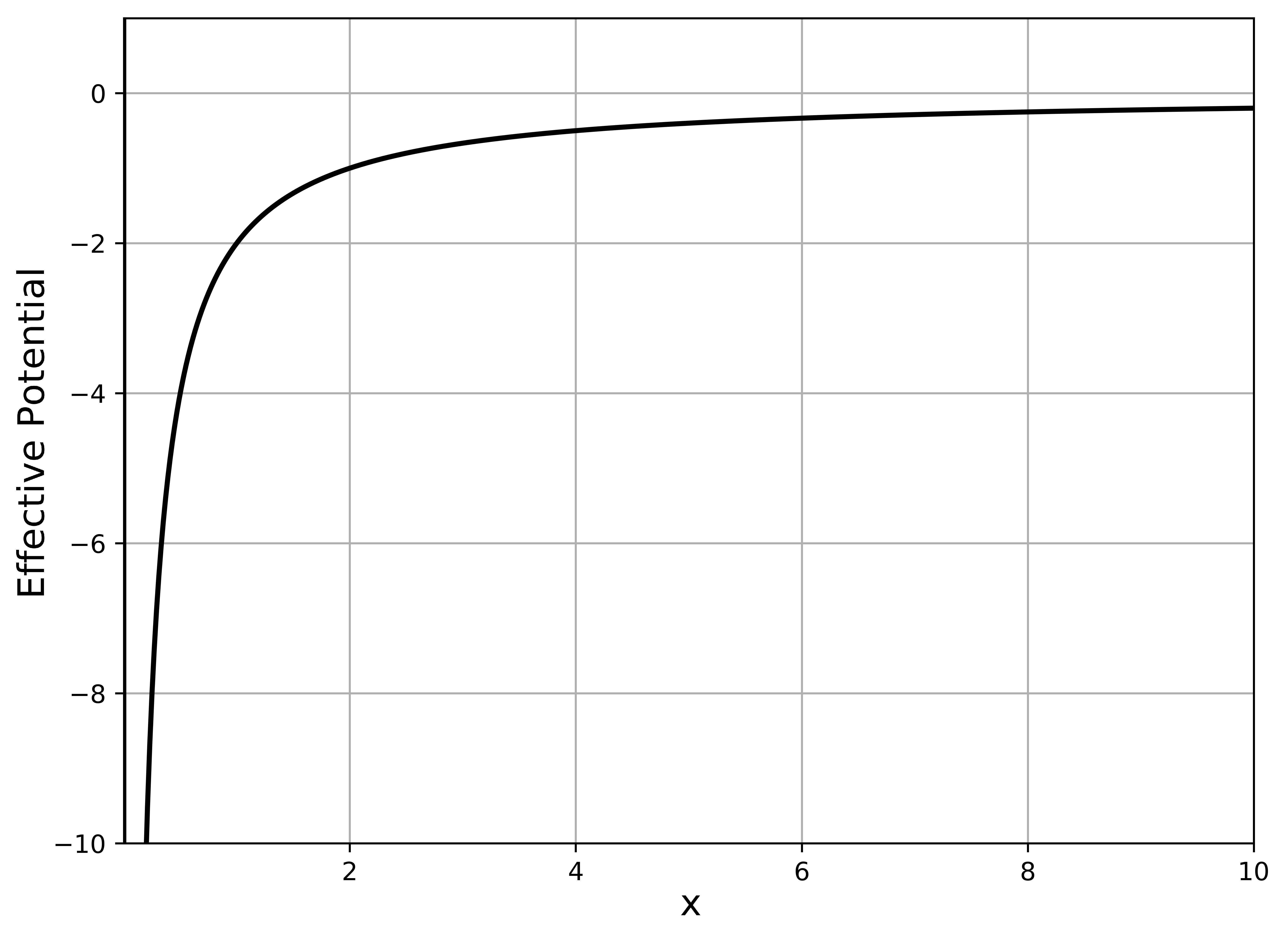
From now on we will introduce the codes necessary to generate the graphs, as well as calculate the normalization of the wavefunctions. First, let’s plot the effective potential graph. During the process of setting the code for different potentials, it is important to know the effective potential in order to adjust the parameters accordingly.
The code above plots the effective potential, as we can see in figure 3
And the graph for the eigenfunctions with an arbitrary normalization, is built by
Which generates the plot shown in the figure 4

As a last step, let’s include in our code, the calculation of the normalization of the wave functions, given by:
Thus, we were able to obtain our final graph, composed of the first three wave functions for the hydrogen atom.

4 Morse Potential
The Morse potential is a common model for the interatomic interaction of a diatomic molecule [11, 12]. In this section, in order to learn how we can use the Phyton code in other problems, we will see what we must change in the code that was made available in the previous section so that the program will be able to solve equation (2) for the quantum number and the Morse potential with arbitrary parameters given by:
| (16) |
In this example, we will calculate the first two bounded states, for that, we must adjust the multiplier for each case as:
And, the most important part, which is the adjustment of the initial data of our problem. Analyzing the effective potential we can verify that the value os parameter must be negative, and its minimum value is zero, so the code must be set as follows:
From now on, the program is able to find the energies of the first two states, which are respectively and . As well as already determined the wave functions also for the first two states.
Then, all that remains is to get all the aesthetic part of the code right, adjusting the limits of graphics, subtitles and other factors. Thus we first get the effective potential, as shown in Figure 6 and finally arrive at the normalized wave functions shown in Figure 7.


In Table 2, we can compare the eigenvalues found by the Numerov’s method with the analytical values given by .
| n | Numerov’s Energy | Analytical value |
|---|---|---|
| 0 | 7.1380 | 7.0 |
| 1 | 15.0380 | 15.0 |
5 Quantum Dot
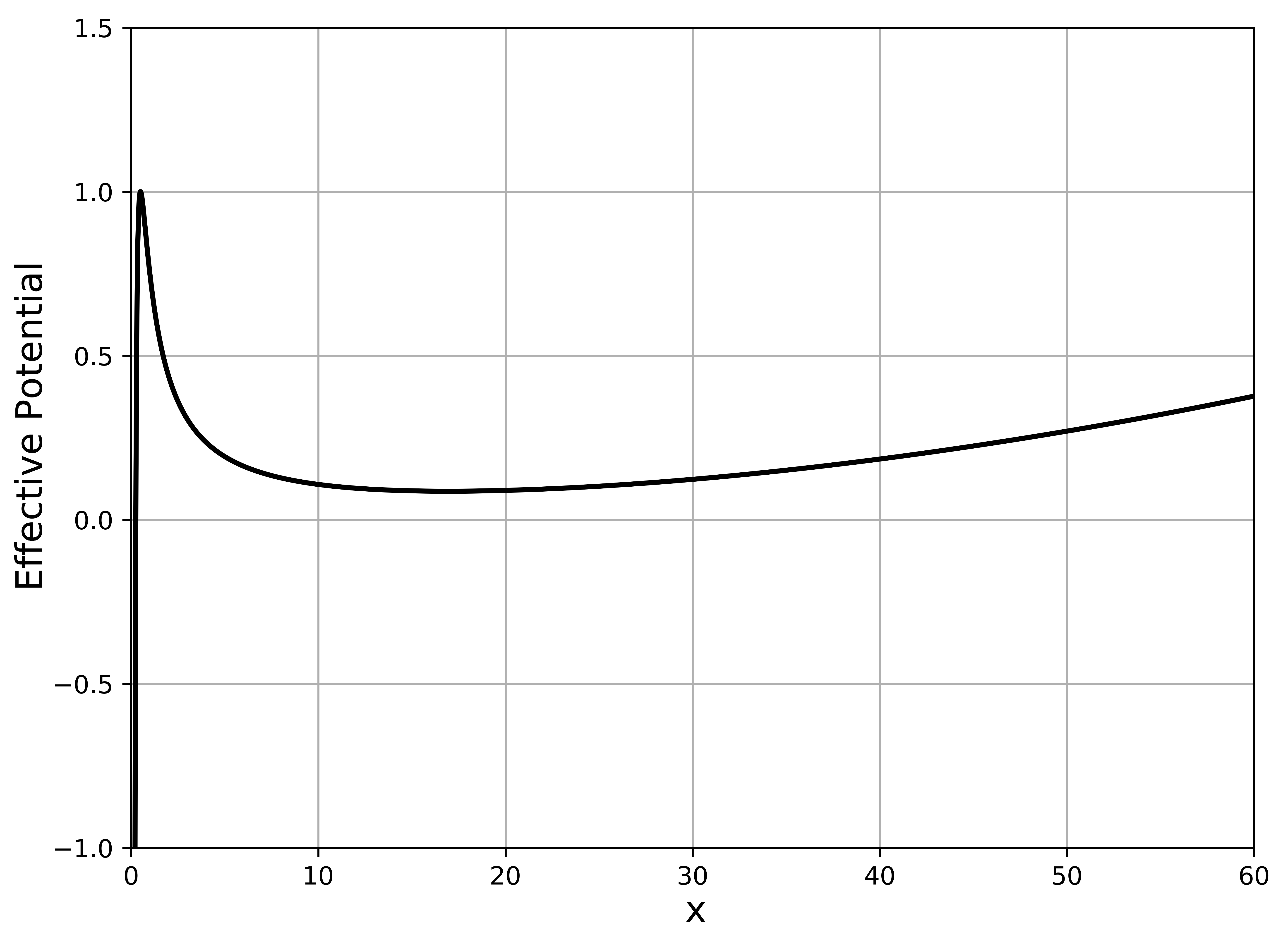
The development of technology based on quantum dots is quite recent, but it is already showing signs that it is the next great technology, when we talk about optics. In a simple model for a quantum dot composed of two electrons, they can be described with a external harmonic oscillator potential of frequency . Following the steps of reference [10], we have the effective potential to be introduced into equation (2) for the quantum number is given by:
| (17) |
introducing this potential into our code, let’s now calculate the first five solutions that the program is capable of finding. We can observe that in our code used so far, we only have up to three wave functions, in this example we will show how we included two more solutions in the code. The procedure is very simple, just add the and functions along the code and all the other parts that are related to them, for example,
Now, as in the previous example, let’s include the multipliers, remembering to include the new wave functions.
And finally, we must include the initial conditions for our problem, as shown below.
Thus, adjusting the rest of the code, we obtain the first five eigenvalues. The effective potential and the eigenfunctions can be seen in Figures 8 and 9.

In Table 3, we can compare the eigenvalues found by the Numerov’s method with the analytical values for the quantum dot given by .
| n | Numerov’s Energy | Analytical value |
|---|---|---|
| 4 | 0.1046 | 0.10 |
| 6 | 0.1403 | 0.14 |
| 8 | 0.1760 | 0.18 |
| 10 | 0.2134 | 0.22 |
| 12 | 0.2507 | 0.26 |
6 Conclusion
Analyzing the results arranged in Tables 1, 2 and 3 we can conclude that the method used here is able to reproduce the analytical results within small errors.
Therefore, it is evident that the numerical method of Numerov is a powerful tool, easy to use, which can help in the development of not only new knowledge in the area of programming, but also the solution of Schrödinger equations outside the usual results found in the examples of modern physics books. We hope that this short introduction to the code, which can be found in full at https://1drv.ms/u/s!Ai_Lqkgh1kiskp5_cfOtwCfqX-LpTw?e=srdmzS, will open doors for students to create their own versions, increasingly improving the versatility of this tool.
Acknowledgment
One of us (FS) was financed in part by the Coordenação de Aperfeiçoamento de Pessoal de Nível Superior – Brazil (CAPES), Finance Code 001.
References
- [1] Caruso, F. & Oguri, V.: Numerov numerical method applied to the Schrödinger equation, Rev. Bras. Ens. Fis. 36, 2310 (2014).
- [2] Numerov, B. V.: A Method of Extrapolation of Perturbations, Month. Not. Roy. Astro. Soc. 84, 592 (1924).
- [3] Numerov, B. V., Note on the numerical integration of , Astronomische Nach. 230, 359 (1927).
- [4] Blatt, J. M.: Practical points concerning the solution of the Schrödinger equation, Jour. Comput. Phys. 1, 382 (1967).
- [5] Allison, A. C.: The numerical solution of coupled differential equations arising from the Schrödinger equation, Jour. Comput. Phys. 6, 378 (1970).
- [6] Leroy, J. P. & Wallace, R.: Renormalized Numerov method applied to eigenvalue equations: extension to include single derivative terms and a variety of boundary conditions, Jour. Phys. Chem. 89, 1928 (1985).
- [7] Bağcı, A. & Güneş, Z.: An efficient approximation for accelerating convergence of the numerical power series. results for the 1d Schrödinger’s equation, arXiv:2111.11379 (2021).
- [8] Caruso, F. & Martins, J. & Oguri, V.: Solving a two-electron quantum dot model in terms of polynomial solutions of a Biconfluent Heun equation, Ann. Phys. 347, 130 (2014).
- [9] Caruso, F. & Martins, J. & Oguri, V. & Silveira, F.: Corrigendum to“solving a two-electron quantum dot model in terms of polynomial solutions of a biconfluent heun equation”[ ann. phys. 347, 130 (2014)], Ann. of Phys. 377, 518 (2017).
- [10] Caruso, F. & Oguri, V. & Silveira, F.: Numerical solutions for a two-dimensional quantum dot model, Braz. J. Phys. 49, 432 (2019).
- [11] Morse, P. M. & Stueckelberg, E. C. G.: Diatomic molecules according to the wave mechanics I: Electronic levels of the hydrogen molecular ion, Phys. Rev. 33, 932 (1929).
- [12] Morse, P. M.: Diatomic molecules according to the wave mechanics. II. Vibrational levels, Phys. Rev. 34, 57 (1929).