Data-Driven, Soft Alignment of Functional Data Using Shapes and Landmarksxiaoyang.guo.fl@gmail.com, {wwu, anuj}@stat.fsu.edu
Abstract
Alignment or registration of functions is a fundamental problem in statistical analysis of functions and shapes. While there are several approaches available, a more recent approach based on Fisher-Rao metric and square-root velocity functions (SRVFs) has been shown to have good performance. However, this SRVF method has two limitations: (1) it is susceptible to over alignment, i.e., alignment of noise as well as the signal, and (2) in case there is additional information in form of landmarks, the original formulation does not prescribe a way to incorporate that information. In this paper we propose an extension that allows for incorporation of landmark information to seek a compromise between matching curves and landmarks. This results in a soft landmark alignment that pushes landmarks closer, without requiring their exact overlays to finds a compromise between contributions from functions and landmarks. The proposed method is demonstrated to be superior in certain practical scenarios.
Keywords: Data-driven alignment, Functional Data Analysis, Phase-Amplitude Separation, Landmark Registration, Square-root Velocity Function
1 Introduction
Functional and shape data analysis is a branch of statistics that seeks tools for statistical analysis of signals, curves, surfaces, or even more complex objects while being invariant to certain shape-preserving transformations. Among the different kinds of objects that one comes across in shape analysis, the simplest types are real-valued functions on a fixed interval. One of the most important problems in functional and shape data analysis is the registration of points across objects. In case of real-valued functions, registration boils down to warping the temporal domain of functions so that geometric features (peaks and valleys) of functions are well-aligned. This task, also called curve registration (Ramsay and Li, 1998; Srivastava et al., 2011), or functional alignment (Ramsay, 2006), or phase-amplitude separation (Marron et al., 2014; Marron et al., 2015) is omnipresent in the functional data analysis and its applications. For example, in analysis of data collected by wearable devices, it is critically important to register time-series data across experiments and observations (Choi et al., 2018). Similarly, in analysis of biological growth data, including the famous Berkely growth data (Tuddenham and Snyder, 1954), the growth bursts (peaks) are located at different times for different subjects and need to be registered across subjects for analysis. In all these cases, a simple cross-sectional statistical analysis based on the norm, and without any alignment, leads to a loss of geometric features and, thus, incorrect inferences (Marron et al., 2015; Srivastava and Klassen, 2016). If one does not account for misalignment in the given data, this can artificially inflate variance and can defeat any statistical analysis, especially the one based on analysis of variance. Registration or alignment is very important for preserving geometric features and to obtain statistics inferences that are more meaningful and interpretable.
In order to formulate the problem, consider a given set of functions: and the goal is to find a set of time warping functions, , such that the warped functions are as well aligned as possible. We will use the terms alignment and registration interchangeably throughout the paper. For simplicity, we restrict the domain to be but any finite interval can be transformed into by a simple translation and scaling. The time warping functions are typically boundary-preserving, positive diffeomorphisms of to itself. The quantification of how well a set of functions are aligned depends, of course, on the application and is open to subjectivity of an observer. However, one does need an objective function for automating the alignment process, especially for handling large volumes of data. There are several objective functions defined in the literature for such alignment. The classical solution is the dynamic time warping (DTW) that has been used extensively in signal, especially speech processing. DTW and related methods are based on minimizing a penalized- distance between aligned functions (Sakoe and Chiba, 1978; Ramsay and Li, 1998). That is, for any pair , , they solve for the optimization problem:
| (1) |
where is a roughness penalty on . For instance, the first-order penalty is and the second-order penalty is . Despite its popularity, this method has some major limitations: (1) The solution is not inverse symmetric in and ; (2) In fact, the objective function is not a proper metric and cannot be used for ensuing statistical analysis; (3) Finally, it maybe difficult to find a balance between the penalty and the data term. This is because the penalty term does not carry any additional information which relates the warping function to the observed data.; it simply imposes arbitrary constraints on the warping function. (This is in contrast to the proposed method where the extra term comes from the additional information present in form of landmarks.) These issues are illustrated using an example in Figure 1 for the two functions , shown in the top panel. The next three rows show the result of alignments under the first order penalty, each obtained using Eqn. 1 but for different values of . In order to study the symmetry of the solution, we perform alignment both ways – to and to – and compose the resulting s. Ideally, if the solution is symmetric, this composition should be identity, the line. We see that when , the solution is symmetric but we have the pinching effect (Marron et al., 2015) in alignment (second row of Figure 1). As increases, the pinching effect is gone but two things happen: (1) there is a decrease in the level of alignment, and (2) the solution is less and less symmetric. Despite its multiple limitations, this is the most commonly-used technique for registration of functional data.

 |
 |
 |
 | |
| and | and | and | ||
 |
 |
 |
 | |
| and | and | and | ||
 |
 |
 |
 | |
| and | and | and |
A recently developed theory (Srivastava et al., 2011; Srivastava and Klassen, 2016) addresses these issues by defining a new mathematical representation of functions, called square-root velocity function (SRVF). For an absolutely-continuous function , its SRVF is defined to be . If is time warped using a warping , resulting in , the corresponding effect on its SRVF is given by , henceforth denoted by the expression . This constitutes the right action of , the group of all time warping functions, on , the set of all SRVFs. For any two functions , , with the associated SRVFs , , the registration problem is then given by . No additional penalty term is needed here making it a fully automatic method. As described later, this formulation: (1) avoids the pinching effect, (2) results in a symmetric solution in terms of and , and (3) the infimum is a proper metric that can be used for statistical analysis. However, this solution has some limitations. Despite its good performance in raw peak alignment, sometimes it is susceptible to overalignment. In case the data is noisy and contains spurious peaks, the solution results in alignment of these spurious peaks with the signal peaks, as shown by an example in Figure 2. This example studies two functions with one tall peak and each and numerous small peaks associated with the noise. The SRVF solution aligns a large peak in one function with a nearby smaller peak, and vice-versa.
One can also introduce a roughness penalty on the time warping functions, similar to Eqn. 1, according to: . The second term is the Fisher-Rao distance (Srivastava and Klassen, 2016) between and identity warping function . However, a penalty simply curtails the amount of warping, irrespective of function shapes, and is seldom useful in handling the issue of over alignment. It will be better if there is some external information available to help overcome the effects of noise.

 |
 |
Hard Landmark Alignment: The external information can come in form of landmarks. These are labeled points in the domain that represent locations of great importance in the functions, e.g., points of high curvature, anatomical landmarks, etc. They represent the same features across functions and it is meaningful to register them. Suppose we are given labeled landmarks ( time points for function ) that denote certain underlying temporal events that need to be aligned during registration. In other words, one wants both and to be aligned as well as possible. Examples of landmark-based registration are presented in (Kneip and Gasser, 1992; Gasser and Kneip, 1995; Bigot, 2006). However, these approaches are essentially hard registration methods in the sense that they insist on matching the landmarks exactly, i.e., variance( for all . After registering all the landmarks using affine transformation actions, the remaining problem is to individually align segments separated by landmarks. One of the drawbacks of any hard registration is that it ignores the global geometry of full functional objects and relies only on local shapes.
Soft Landmark Alignment: In contrast, if the landmarks are steered closer to each other, but without requiring them to overlay each other, then it is called soft matching, or a landmark-guided functional or shape data analysis (Kurtek et al., 2013; Bauer et al., 2015). What is the motivation for soft registration? Since one usually estimates the landmarks from the data, either manually or automatically, landmarks themselves may have errors, and the resulting hard registration can be erroneous. Moreover, if one has multiple choices of landmarks, the hard registration has to select only one solution, while ignoring the other possibilities. All this motivates the need for a data-driven soft registration, in order to reach a more reasonable solution. It is termed data-driven because one determines the relative strengths of contributions from the function shape and landmarks from the data itself.
In recent years, there have also been some Bayesian framework for function alignment, see e.g., (Telesca and Inoue, 2008; Cheng et al., 2016; Kurtek et al., 2017; Lu et al., 2017). However, current Bayesian approaches do not consider incorporating extra landmark information but rather focus on global curve registration. Moreover, the disadvantage of Bayesian methods is the computational cost and the dependence of the solution on the prior models.
We propose an extension of the SRVF framework that incorporates landmark information in a soft fashion. This two-step procedure: (1) time warps the given functions or curves into hard alignment, and (2) performs further warping using a penalized elastic metric. We first introduce it for pairwise alignment and then naturally extend it for multiple alignment. The main strengths of this framework as as follows:
- 1.
Optimal Combination of Shapes and Landmarks: It combines information from function shapes and landmark locations, and results in an optimal alignment solution. It provides a solution that lies between fully constrained (hard registration) and fully unconstrained. The choice of relative weights of the two terms is based on cross-validation and, hence, the whole framework is data driven.
- 2.
Mathematical Properties: The cost function used for soft registration has nice mathematical properties – it is non-negative, symmetric, and satisfies the triangle inequality, i.e., it is a pseudometric! Consequently, this pseudometric can be used for statistical analysis of functional data. This provides a consistency between the metric used for registration and metric used in statistical analysis.
- 3.
Computational Efficiency: The solution to the proposed soft alignment is computationally efficient, as it uses the fast dynamic programming algorithm for alignment. Code is available on Github: https://github.com/xiaoyangstat/soft-alignment-of-functional-data-using-shapes-and-landmarks
The rest of this paper is organized as follows. Section 2 briefly summarizes the SRVF framework and introduces a penalized elastic pseudometric for soft landmark alignment. Section 3 extends this pairwise soft landmark alignment to multiple functions. In Section 4, we present a variety of results on both simulated data and real data to demonstrate the superiority. Finally, Section 5 provides concluding discussions and future directions.
2 Soft Landmark Alignment
In this section, we first introduce the SRVF framework for unconstrained alignment and then discuss the hard alignment, or the fully constrained approach. Then, we introduce the framework for intermediate constraint or soft alignment of two functions given their landmark data. Before we discuss different options, we outline some important desirable properties that a soft framework should provide.
- 1.
Landmark Guidance: The framework should obviously be able to incorporate both sets of information: functional shapes and landmarks, in performing time warping and registration. Ideally, the user should be able to estimate the relative weights of these components using the data itself.
- 2.
Metric or Pseudometric: The objective function for pairwise registration of functions should be symmetric in the two input variables. In other words, the registration of to under this criterion will be compatible with the registration of to . Furthermore, if the objective function is non-negative and satisfies triangle inequality, then it can be used as a proper metric in the ensuing functional data analysis. Even if it is not a full metric, but just a pseudometric, it can still be useful in statistical analysis of registered functions.
- 3.
Invariance Condition: It is important to note that an identical warping of any two functions preserves their registration. In other words, for any time warping function , the registration between and is the same as the registration between and , for any . Therefore, the objective function used for registration should also be invariant to simultaneous warping. This requires that the associated metric or pseudo-metric preserves its value under the action of time warping.
As we introduce different options for soft registration, we will evaluate them using these desired properties.
2.1 Unconstrained SRVF Alignment
Our approach is to modify an SRVF-based technique for elastic registration and shape comparison. So we start by briefly introducing the SRVF framework. For details, please refer to the textbook (Srivastava and Klassen, 2016). Let be an absolutely continuous function on and let be the set of all such functions. Define the square-root velocity function (SRVF) of an to be the function , where . It can be shown that this map provides a bijective mapping between and , up to an addition by a constant. In fact, one can reconstruct from the pair using . Let denote the set of all boundary-preserving positive diffeomorphisms of to itself; forms a group with the group operation given by composition, and the identity element being . The group acts on from right by composition , and the corresponding action of on the SRVF space () is given by ; we will denote it by . It can be shown that the metric in the space of SRVFs is exactly the Fisher-Rao distance in (Srivastava and Klassen, 2016). Furthermore, under this metric, the group action of preserves the distance, i.e., for any and , we have , where denotes the norm. Consequently, the problem of pairwise alignment can be formulated as finding the optimal warping according to:
| (2) |
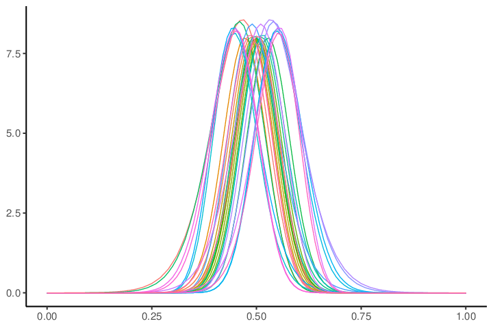
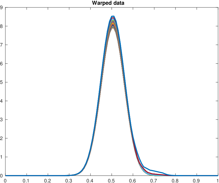
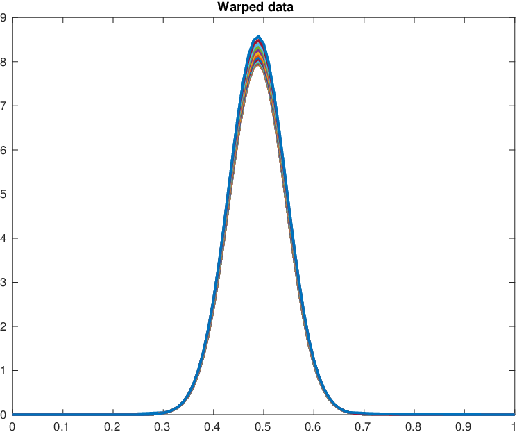
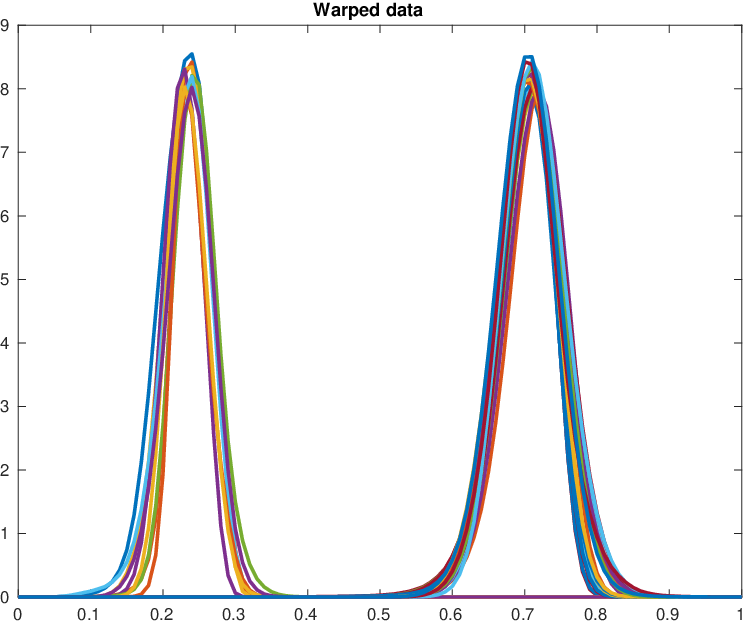
This minimization problem can be solved efficiently albeit approximately using the Dynamic Programming algorithm (DPA). Figure 3 shows an example of this framework applied to the alignment of multiple functions. The left panel shows a set of given functions . On the right hand side, we compare different alignment methods. The top row shows the aligned functions and the bottom row shows the warping functions such that . From left to right, the results are from -based (Ramsay et al., 2021), SRVF-based (Eqn. 1), -based (Our implementation of Eqn. 2), Bayesian approach (Lu et al., 2017) implemented in (Tucker, 2022), -based (Tang and Müller, 2008). In addition to DPA for SRVF matching, an exact matching algorithm based on the change points of functions has also been developed for this setup (Robinson et al., 2017).
 |
 |
 |
 |
 |
 |
 |
 |
 |
 |
 | |
| Ramsay et al., 2021 | SRVF | Lu et al., 2017 | Tang and Müller, 2008 |
As mentioned earlier, while this technique is impressive in alignments of peaks and valleys on the given functions, it is also susceptible to noise and over-alignment. Since one can potentially use the landmark information, if available, to overcome this issue, we turn our attention to the problem of incorporating landmark information in the registration process. The landmarks can be the locations of critical points or any other meaningful geometric features of given functions. Registered landmarks can often assist in alignment and lead to a more meaningful phase-amplitude separation, relative to the unconstrained problem. These landmarks can be obtained in different ways depending on the data and the context (Ramsay, 2006), but here we shall assume that a set of sparse landmarks is given.
2.2 Pairwise Hard Landmark Alignment
The SRVF framework, as defined originally, is not designed to incorporate landmark information in the matching problem but has been extended in recent years to a hard matching (Strait and Kurtek, 2017; Strait et al., 2017; Bharath and Kurtek, 2017; Strait et al., 2018). We will first discuss the hard alignment, i.e., the solutions where the landmarks are to be matched precisely with each other. Later on, we will relax this constraint to reach the soft alignment.
In the following discussion, we will assume that all functions come with the same number of ordered landmarks and are in one-to-one correspondence. Suppose a function has associated landmarks: , where . A mathematical representation of with landmarks is given by : , where . Also, denotes the SRVF of , as earlier. The action of the warping group on the pair is given by ; note that this action preserves the number and the ordering of the landmarks.
Let be the set of landmarks of and be the landmarks of . Rather than matching these landmarks to each other, we will choose a third set, called the reference landmarks , and match to this reference set. The reference set is sometimes predefined from the problem context and is kept fixed through out the process. If not, we can choose the reference set from the given data. For example, one can pick one of two given sets of landmarks, or compute arithmetic average of the two. (Note, if the reference landmarks depend on the data, as opposed to being pre-determined and fixed, we will lose a nice theoretical property of invariance as explained later.) Now, the goal of pairwise hard alignment is to find warping functions such that: (1) and , which means that one matches the landmarks exactly; and, (2) match features (peaks and valleys) of the two functions in the corresponding subintervals.
To motivate the second item, note that problem is ill defined if we only care about registering landmarks and ignore the shapes of functions. Given , and their landmarks and , the sets and have infinitely many elements. To narrow down the solution space, one can restrict the to be piecewise linear. Although this solution is simple, it completely ignores the shapes of functions and leads to badly registered functions. Therefore, in addition to the landmark matching, one also requires the functions to be optimally registered to each other in the corresponding subintervals. Towards that goal, one can simply apply the SRVF framework, discussed above for the full interval , to each of the matched subintervals independently. The detailed steps are as follows:
- 1.
Select the reference landmarks , either from the problem context or from the data. Partition the time domain into subintervals with landmarks as boundaries, for each function. This defines the boundary points of the warping functions , .
- 2.
Align the respective functions on these subintervals separately using the SRVF framework. Concatenate the warping functions over these intervals to form full time warping functions over . Call them .
- 3.
Optionally, center the warping function according to , where .
We present an example of this approach in Figure 4 using a single landmark. The two functions: (multimodal) and (unimodal), are as shown on the left. The landmark for is the location of its last peak while the landmark for is the location of its only peak. The reference landmark is chosen to be the same as the landmark of . The result of hard registration is shown in the middle panel, where landmarks as well as the corresponding functions in the two subintervals are matched perfectly. An example with real data is presented in Figure 5, which shows two spiking activities of a movement-encoded neuron in the primary motor cortex, taken from (Wu and Srivastava, 2011). The two spike activities and are equipped with landmarks that are marked as green and black circles. We would like to align both the functional shapes as well as the landmarks. As the top row of Figure 5 shows, the unconstrained alignment by SRVF does not register landmarks correctly. However, by using hard registration, one can see in the bottom row that the landmarks are perfectly aligned.
 |
 |
 |
 |
 |
 |
|---|---|---|
 |
 |
2.3 Pairwise Soft Landmark Alignment
While hard alignment provides us with a way of incorporating landmarks information to alignment, it relies too heavily on the locations of the landmarks. The result can be misleading in situations where the landmarks are not precise. Thus, we want to pursue a soft approach that can balance the contributions of landmarks and function shapes. Unlike hard registration, a soft alignment does not require matched landmarks to be aligned exactly but pushes them towards each other. In summary, soft alignment seeks intermediate solutions between unconstrained alignment (Section 2.1) and hard alignment (Section 2.2).
We remind the reader that it is desirable to perform matching using an objective function that is either a proper metric or a pseudometric. That is, the desired cost function should satisfy non-negativity, identity of indiscernibles (for a metric), symmetry and triangle inequality. This, in turn, requires that we have invariance of the objective function under the group action of time warping (refer to the proof in appendix).
Now we are ready to present our approach for soft alignment. The basic idea is to perform pairwise alignment in two steps: (1) First, we perform hard registration to match the shapes and landmarks of the given functions. (2) Then, using the resulting functions, we perform a further penalized SRVF alignment. That is, we minimize the SRVF objective function along with a term that forces the additional warping function to stay close to the identity. This second part is essentially a search in without any additional involvement of landmarks but constrained to stay closed to . Depending on the choice of a tuning parameter , one can sweep the entire spectrum of solutions ranging from hard registration ( very high) to fully unconstrained SRVF registration (). We will describe how the propose soft alignment is superior in term of both theory and computation to the previous ideas.
To define the objective function mathematically, start with any two functions , with SRVFs and , and respective landmarks and , Let and be the optimal warping functions resulting from the hard registration discussed previously (Section 2.2). The individual landmarks are thus perfectly aligned to the reference landmarks .
Definition 1
(Pairwise Soft Landmark Registration) In the setting described above, define the optimization problem for soft landmark, pairwise function registration to be:
| (3) | |||||
where is a constant function with value one.
The positive constant is a tuning parameter that can be used to control the influence of the landmarks on the overall solution. What is the motivation for using the objective function suggested here? Here are some properties that makes this choice meaningful.
- 1.
Difference from Eqn. 1: Even though this formulation takes the form of a penalized alignment, it is fundamentally different from the formulation in Eqn. 1. Here, the default solution (without any alignment by ) is hard SRVF alignment, while in Eqn. 1 the default solution is no alignment. Here, is being used to reduce local alignment (without constraint) and move towards a global (with constraint) alignment. In Eqn. 1, is being used to perform all alignment – local and global.
- 2.
Pseudometric nature: The optimization leads to a pesudo-metric for ensuing statistical analysis of functions.
Lemma 1
The resulting infimum of the objective function in Eqn. 3, call it , is a pseudometric on the space .
Proof: See appendix. Consequently, this objective function is symmetric and it satisfies triangle inequality.
- 3.
Invariance condition: An important property of this pseudometric is the following.
Lemma 2
The action of on joint space , given by preserves for a fixed reference landmark . That is,
for all and .
Proof: Suppose and are the time warping functions from hard registration for and . For an arbitrary , the new time warping functions for hard registration of and are and , respectively. Therefore,
- 4.
Balance between hard and unconstrained registration: When , the resulting distance is exactly the same as cost function used in Eqn. 2 for unconstrained alignment. As increases, the impact of landmarks on the alignment increases, and eventually when becomes very large then tends to , resulting in a purely hard registration. For intermediate s, we get solutions that represent combinatiosn of these two solutions.
Selecting Using Cross Validation: The choice of the relative contributions of two terms, controlled by , is important in reaching a good solution. This choice depends on the application, the data and the end-user. In addition, one can automate the process using cross-validation. We will use some examples in Section 3.1 to discuss this issue further.
3 Soft Landmark Alignment of Multiple Functions
Now we consider the problem of alignment of multiple functions, each equipped with their own landmarks. This multiple alignments is based on the repeated use of the pairwise alignment framework derived previously. The basic idea is to use , a pseudometric on space, to define a ’consensus’ function, and use this consensus as a template to align individual functions to this template.
Let , with fixed landmark , denote the consensus, defined as follows. We are given individual SRVFs with respective landmarks . Define the landmarks of the consensus in some pre-determined fashion, for instance, using landmarks from one of given function; call them . Then, the consensus function (in the SRVF space) is defined to be:
| (4) |
while keeping fixed. (We call this function consensus instead of a mean because we don’t have a full metric but only a pseudometric on the representation space.) We solve this optimization problem iteratively as follows. First we perform a hard registration of each to the current estimate (note that is kept fixed in these iterations). After the hard registration, Eqn. 4 is reduced to a penalized SRVF multiple alignment problem:
where is already pre-computed from the hard registration. Then, for fixed , . The overall algorithm for soft registration of multiple functions is given as in Algorithm 1.
Given functions and the associated landmark vectors .
This is an iterative algorithm and one needs to consider its convergence properties. Since the algorithm is based on alternative optimization over and , the convergence to a global solution is not guaranteed. At best, one expects a local solution solution from this optimization. Algorithm 1 returns soft-aligned functions , in which landmarks are pushed together but not necessarily registered.
3.1 Selection of by Cross Validation
The relative contribution of landmarks and functions’ shapes is controlled by , so the choice of becomes an important factor. In case is to be chosen automatically from the data, we propose to use leave-one-out cross validation (LOOCV) as follows:
where is the time warping function from hard registration (Step 2 of Algorithm 1) and is the additional warping (Step 3 of Algorithm 1). The intuition is to find the such that the resulting consensus is the center of the shape distribution of functions. Given a fixed , we first leave a function out and calculate the consensus of the remaining functions using Algorithm 1. This consensus acts as the estimate for , and we compute the difference in the shape of and its estimate. Total error over all functions makes up the objective function for selecting . We use grid search over an interval to find the optimal .
We demonstrate this idea using two simulated but extreme examples.
- 1.
Completely Arbitrary Landmarks: We create 5 functions using for different s. We select the midpoint as the landmark for all functions, irrespective of their shapes. Thus, the landmarks do not contain any useful information. We use the LOOCV procedure to find the best and results are shown in Figure 6. As expected, the best is found to be , implying that landmarks actually do not help and are discarded.
(a) Raw Simulated Functions (b) Hard Registration (c) Unconstrained Registration (d) LOOCV Shape Error (e) Time Warping Functions in Hard Registration (f) Additional Time Warping Functions, Figure 6: Selecting best based on LOOCV shape error when landmarks are meaningless - 2.
Precise Landmarks: This time we create some multimodal functions and pick the locations of third peak as landmarks in each functions. In addition, these functions are corrupted by additive white Gaussian noise. We compute soft alignment experiments, and show the results in Figure 7. In this case, the unconstrained alignment fails to register the correct peaks, and LOOCV shape error points to the large that approximates hard registration. Incidentally, there are two near-optimal values of and they both lead to similar alignment results.
(a) Raw Simulated Functions (b) Unconstrained Alignment (c) Soft Alignment, (d) LOOCV Shape Error (e) Hard Registration Warpings (f) Additional Warping, Figure 7: Selecting best based on LOOCV shape error when landmarks are meaningful
4 Experiment and Applications
Next, we will present some experimental results involving both simulated as well as the real data to demonstrate the proposed method.
4.1 Synthetic Data
The top left panel of Figure 8 shows two simulated functions, and formed by superimposing some Gaussian density functions. The function has five peaks while the has one peak. We select the last peak of and the only peak of as a single landmark for each function. We first pre-align two sets of landmarks using hard registration, as shown in the top row. Next, for different values of the tuning parameter , we obtain different soft alignments as shown in the middle. From left to right, the value of is increasing, causing a steady increase in the influence of the landmarks. As we can see, the landmark of goes through every peak of for different .
In the second simulated scenario, we focus on the soft nature of the solution for the multiple alignment. The left panel of Figure 9 shows five simulated functions, each with two landmarks each marked by vertical dashed lines. The corresponding segments across functions are colored in the same way: blue, red and yellow. The pre-alignment is given by hard registration, which can be seen in the middle panel. As we increase , the resulting standard deviation of two sets of landmarks is plotted in the right panel. It goes from a large value to 0, implying the alignment is changed from unconstrained alignment to hard registration. The intermediate values represent soft alignment solutions.
4.2 Real Data
Now we show three examples of soft alignment using real data. We also show results from a hard landmark alignment method (Ramsay et al., 2021) for comparison.
Fourier-transform infrared spectroscopy (FTIR) Data:
The first application is from Fourier-transform infrared spectroscopy (FTIR) data
studied in (Srivastava, 2017).
FTIR is widely used in geology, chemistry, materials, and biology to
to measure infrared absorption and emission spectra of a solid, liquid or gas,
and to characterize material properties.
The dataset contains 10 observations and each observation contains the changes in transmittance as a function of wavelength.
The common pattern in this data is that all functions have three major peaks that are expected to be matched.
However, there are often some small noise peaks in the data because of experiment conditions
such as instrument calibration, specimen contamination, and so on.
Due to the existence of numerous small
peaks, the unconstrained alignment fails to match the three major peaks with each other, as
shown in Figure 10(c).
In order to assist with the alignment, we select landmarks representing the three major peaks.
The landmarks are not guaranteed to be precise thus hard landmarks registration is a strong constraint, as shown in Figure 10(d).
Figure 10(b) illustrates the result of soft alignment, which reflects the common pattern of these functions.
As we can see, the landmarks of the second and the third peak are not matched exactly while for the first peak, they are precisely registered.
In this case, provides the smallest prediction of LOOCV Shape error. The resulting mean functions from soft alignment and hard alignment show the three major patterns while the one from unconstraint alignment has more undesired small peaks.
| (a) Raw Data | (b) Soft Alignment, | (c) Unconstrained Alignment | (d) Ramsay et al., 2021 |
| (e) LOOCV Shape Error | (f) Additional Warpings, | (g) Unconstrained Time Warpings | (h) Ramsay et al., 2021 |
Tallahassee Electricity Data: The next example involves daily household electricity consumption profiles for homes in Tallahassee, FL, USA (Dasgupta et al., 2019). We select 75 households from a neighborhood and for each household, the data shows the daily electricity consumption (on weekdays). The common pattern of these functions is bimodal, because of the typically high consumptions in the mornings and evenings. However, the unconstrained alignment does not result in a bimodal pattern, as shown in (c), due to the presence of multiple small peaks. To apply landmark registration, we automatically select the locations of largest peaks in the first and second half of domain as landmarks. The resulting soft alignment result is presented in (b), where are obtained in (d). Looking at mean functions, unconstrained alignment shows many smaller peaks and valleys while soft alignment exhibits a prominent bimodal pattern, reflecting the utility consumption pattern of the neighborhood. The hard landmark registration also shows a bimodal mean. However, the mean function seems to over flat for the smaller peaks. Most importantly, the LOOCV curve explains that soft alignment achieves lowers shape error.
| (a) Raw Data | (b) Soft Alignment, | (c) Unconstrained Alignment | (d) Ramsay et al., 2021 |
| (e) LOOCV Shape Error | (f) Additional Warpings, | (g) Unconstrained Warpings | (h) Ramsay et al., 2021 |
Precipitation Data: The last example relates to annual precipitation of 10 European countries. As we know, the peaks and valleys of precipitation will not be temporally synchronized across different countries. To study the common structure of the precipitation for those countries, we need to remove or reduce the phase variability through alignment. We select the largest peak as landmarks, represented by green circles in Figure 12. As before, we balance the result between unconstrained alignment and hard registration with (from LOOCV) and get the soft alignment. This is shown in (b) of Figure 12. Comparing with the cross-sectional mean, mean pattern from both soft alignment and unconstrained alignment displays more prominent peaks and valleys. In addition, soft alignment preserves the largest peak not captured in the unconstrained alignment.
| (a) Raw Data | (b) Soft Alignment, | (c) Unconstrained Alignment | (d) Ramsay et al., 2021 |
| (e) LOOCV Shape Error | (f) Additional Warpings, | (g) Unconstrained Warpings | (h) Ramsay et al., 2021 |
5 Summary
In this work, we have presented a novel approach to incorporate landmarks into elastic functional alignment. The strength of this data-driven approach is that it allows one to balance the contributions of landmarks and function shapes in reaching an optimal registration. This is useful when alignment based purely on the geometry of functional data is not reliable, and some additional information in form of landmarks is present. In those cases, soft alignment can help provide a more meaningful solution.
The objective function for soft alignment is actually a pseudometric and lends itself nice theoretical properties – non-negativity, symmetry and invariance – to the alignment solution. One can use this pseudometric for subsequent data analysis, such as clustering, principal component analysis, modeling functional data, and functional linear regression. We also note that although this work is limited to alignment of real-valued functions, this framework is directly applicable to curves in any Euclidean space.
6 Appendix
Proof of lemma 1: We need to establish the following properties of :
- 1.
Non-negativity: . This holds because each of the components in is non-negative.
- 2.
Identity of indiscernibles: ; Unlike a metric space, points in a pseudometric space need not be distinguishable. If , then , and this implies and are in the same orbit. In this situation, there will be two different scenarios. One the one hand, if , this implies . One the other hand, if at least one landmarks is different, then . However, in terms of alignment, means alignment is done by the pre-alignment.
- 3.
Symmetry: . The proof uses the isometric property, as shown in Lemma 2.
- 4.
Triangle Inequality: . The proof also uses Lemma 2.
The LHS is less than or equal to the RHS for all . Then . Besides, the above equation is true for all . So
References
- Bauer et al., (2015) Bauer, M., Eslitzbichler, M., and Grasmair, M. (2015). Landmark-guided elastic shape analysis of human character motions. arXiv preprint arXiv:1502.07666.
- Bharath and Kurtek, (2017) Bharath, K. and Kurtek, S. (2017). Partition-based sampling of warp maps for curve alignment. arXiv preprint arXiv:1708.04891.
- Bigot, (2006) Bigot, J. (2006). Landmark-based registration of curves via the continuous wavelet transform. Journal of Computational and Graphical Statistics, 15(3):542–564.
- Cheng et al., (2016) Cheng, W., Dryden, I. L., Huang, X., et al. (2016). Bayesian registration of functions and curves. Bayesian Analysis, 11(2):447–475.
- Choi et al., (2018) Choi, H., Wang, Q., Toledo, M., Turaga, P., Buman, M., and Srivastava, A. (2018). Temporal alignment improves feature quality: an experiment on activity recognition with accelerometer data. In Proceedings of the IEEE Conference on Computer Vision and Pattern Recognition Workshops, pages 349–357.
- Dasgupta et al., (2019) Dasgupta, S., Cordova, J., Arghandeh, R., and Srivastava, A. (2019). Clustering household electrical load profiles using elastic shape analysis. IEEE Powertech,Accepted for Publication.
- Gasser and Kneip, (1995) Gasser, T. and Kneip, A. (1995). Searching for structure in curve samples. Journal of the american statistical association, 90(432):1179–1188.
- Kneip and Gasser, (1992) Kneip, A. and Gasser, T. (1992). Statistical tools to analyze data representing a sample of curves. The Annals of Statistics, pages 1266–1305.
- Kurtek et al., (2017) Kurtek, S. et al. (2017). A geometric approach to pairwise bayesian alignment of functional data using importance sampling. Electronic Journal of Statistics, 11(1):502–531.
- Kurtek et al., (2013) Kurtek, S., Srivastava, A., Klassen, E., and Laga, H. (2013). Landmark-guided elastic shape analysis of spherically-parameterized surfaces. Computer Graphics Forum, 32(2pt4):429–438.
- Lu et al., (2017) Lu, Y., Herbei, R., and Kurtek, S. (2017). Bayesian registration of functions with a gaussian process prior. Journal of Computational and Graphical Statistics, 26(4):894–904.
- Marron et al., (2014) Marron, J. S., Ramsay, J. O., Sangalli, L. M., and Srivastava, A. (2014). Statistics of time warpings and phase variations. Electron. J. Statist., 8(2):1697–1702.
- Marron et al., (2015) Marron, J. S., Ramsay, J. O., Sangalli, L. M., Srivastava, A., et al. (2015). Functional data analysis of amplitude and phase variation. Statistical Science, 30(4):468–484.
- Ramsay, (2006) Ramsay, J. O. (2006). Functional data analysis. Wiley Online Library.
- Ramsay and Li, (1998) Ramsay, J. O. and Li, X. (1998). Curve registration. Journal of the Royal Statistical Society: Series B (Statistical Methodology), 60(2):351–363.
- Ramsay et al., (2021) Ramsay, J. O., Wickham, H., Graves, S., and Hooker, G. (2021). fda: Functional data analysis. R package version.
- Robinson et al., (2017) Robinson, D., Duncan, A., Srivastava, A., and Klassen, E. (2017). Exact function alignment under elastic riemannian metric. In Graphs in Biomedical Image Analysis, Computational Anatomy and Imaging Genetics, pages 137–151. Springer.
- Sakoe and Chiba, (1978) Sakoe, H. and Chiba, S. (1978). Dynamic programming algorithm optimization for spoken word recognition. IEEE transactions on acoustics, speech, and signal processing, 26(1):43–49.
- Srivastava, (2017) Srivastava, A. (2017). Automated alignment of mass spectrometry data using functional geometry. In Statistical Analysis of Proteomics, Metabolomics, and Lipidomics Data Using Mass Spectrometry, pages 23–43. Springer.
- Srivastava and Klassen, (2016) Srivastava, A. and Klassen, E. P. (2016). Functional and shape data analysis. Springer.
- Srivastava et al., (2011) Srivastava, A., Wu, W., Kurtek, S., Klassen, E., and Marron, J. (2011). Registration of functional data using fisher-rao metric. arXiv preprint arXiv:1103.3817.
- Strait et al., (2018) Strait, J., Chkrebtii, O., and Kurtek, S. (2018). Automatic detection and uncertainty quantification of landmarks on elastic curves. Journal of the American Statistical Association, pages 1–35.
- Strait and Kurtek, (2017) Strait, J. and Kurtek, S. (2017). A novel algorithm for optimal matching of elastic shapes with landmark constraints. In Image Processing Theory, Tools and Applications (IPTA), 2017 Seventh International Conference on, pages 1–6. IEEE.
- Strait et al., (2017) Strait, J., Kurtek, S., Bartha, E., and MacEachern, S. N. (2017). Landmark-constrained elastic shape analysis of planar curves. Journal of the American Statistical Association, 112(518):521–533.
- Tang and Müller, (2008) Tang, R. and Müller, H.-G. (2008). Pairwise curve synchronization for functional data. Biometrika, 95(4):875–889.
- Telesca and Inoue, (2008) Telesca, D. and Inoue, L. Y. T. (2008). Bayesian hierarchical curve registration. Journal of the American Statistical Association, 103(481):328–339.
- Tucker, (2022) Tucker, J. D. (2022). fdasrvf matlab. https://github.com/jdtuck/fdasrvf_MATLAB.
- Tuddenham and Snyder, (1954) Tuddenham, R. D. and Snyder, M. M. (1954). Physical growth of california boys and girls from birth to eighteen years. Publications in child development. University of California, Berkeley, 1(2):183.
- Wu and Srivastava, (2011) Wu, W. and Srivastava, A. (2011). An information-geometric framework for statistical inferences in the neural spike train space. Journal of Computational Neuroscience, 31(3):725–748.