跳到论文正文
W Papers独立论文阅读器 arXiv:2203.14501 论文正文 计算阅读时间 · 0%
引用这篇论文根据当前论文元数据生成,正式投稿前建议核对。


License: arXiv.org perpetual non-exclusive license
arXiv:2203.14501v1 [cs.IT] 28 Mar 2022

Space-Time Block Coded Reconfigurable Intelligent Surface-Based Received Spatial Modulation

Ferhat Bayar    Onur Salan    Haci Ilhan    Senior       Erdogan Aydin Thanks: F. Bayar and O. Salan are with the Scientific and Technological Research Council of Turkey (TUBITAK), Kocaeli, Turkey (e-mails: ferhat.bayar@tubitak.gov.tr, onur.salan@tubitak.gov.tr). Thanks: H. Ilhan is with the Department of Electronics and Communications Engineering, Yildiz Technical University, Istanbul, 34220, Turkey, e-mail: ilhanh@yildiz.edu.tr (Corresponding author: Hacı Ilhan). Thanks: E. Aydin is with the Department of Electrical and Electronics Engineering, Istanbul Medeniyet University, Istanbul 34857, Turkey (e-mail: erdogan.aydin@medeniyet.edu.tr)
Abstract

Reconfigurable intelligent surface (RIS) structures reflect the incident signals by adjusting phase adaptively according to the channel condition where doing transmission in order to increase signal quality at the receiver. Besides, the spatial modulation (SM) technique is a possible candidate for future energy-efficient wireless communications due to providing better throughput, low-cost implementation and good error performance. Also, Alamouti’s space-time block coding (ASBC) is an important space and time coding technique in terms of diversity gain and simplified ML detection. In this paper, we proposed the RIS assisted received spatial modulation (RSM) scheme with ASBC, namely RIS-RSM-ASBC. The termed RIS is portioned by two parts in the proposed system model. Each one is utilized as an access point (AP) to transmit its Alamouti coded information while reflecting passive signals to the selected received antenna. The optimal maximum likelihood (ML) detector is designed for the proposed RIS-RSM-ASBC scheme. Extensive computer simulations are conducted to corroborate theoretical derivations. Results show that RIS-RSM-ASBC system is highly reliable and provides data rate enhancement in contrast to conventional RIS assisted transmit SM (RIS-TSM), RIS assisted transmit quadrature SM (RIS-TQSM), RIS assisted received SM (RIS-RSM), RIS assisted transmit space shift keying with ASBC (RIS-TSSK-ASBC) and RIS-TSSK-VBLAST schemes.

Index Terms: 
Space time block coding, Alamouti’s scheme, performance analysis, reconfigurable intelligent surface (RIS), spatial modulation (SM), maximum likelihood (ML).

I Introduction

According to Cisco, all mobile traffic worldwide will reach 77 exabytes per month by the end of 2022. In this context, 5G, which provides enhanced mobile broadband, ultra-reliable and low-latency communications and massive machine-type communications were completed in June 2018. While mmWave and orthogonal frequency-division multiplexing (OFDM) efforts increase to meet 5G standard targets, it has been determined that there is no single technology that can support 5G application requirements [1]. Therefore, the researchers have started studies about new technologies such as non-orthogonal multiple access (NOMA), multiple-input and multiple-output (MIMO), terahertz communication [2], which will form the basis of 6G technology. The key performance metrics of 6G aims to meet are spectrum and energy efficiency, ultra-reliable low-latency communication, coverage and mobility, as well as providing intelligent and dynamic systems that quickly adapt to changing environmental conditions and application types [3]. In this context, schemes such as media-based modulation [4, 5, 6], spatial modulation (SM) [7] and space shift keying (SSK) [8] use reconfigurable antenna to get rich scattering environments. SM and SSK techniques have been presented with other techniques due to index modulation’s (IM) spectral and energy efficiency. The NOMA-based SM scheme provides increased spectral efficiency without additional complexity. Generalized code index modulation (GCIM) aided SM (GCIM-SM) scheme is proposed to increase the communication system’s energy efficiency and data rate while reducing energy consumption [9]. Also, in the literature, there are working about the cooperative protocol [10] and physical layer security system [11] which work with IM techniques to improve overall system error performance.

The researchers focused on the controlling propagation environment to improve the quality of service (QoS) using intelligent reflecting surfaces. The reconfigurable intelligent surface (RIS) scheme uses a large number of small, low-cost and passive reflecting elements. The RIS adjusts the phase of the incident signal and then reflects it to the destination without any energy source [12]. In [13], the researcher proposed RIS aided SSK (RIS-SSK) and RIS based SM (RIS-SM) schemes in collaboration with IM systems on the RIS scheme. Also, [13] and [14] provide the error performance analysis of RIS-based IM over the Rayleigh fading channel and Weibull fading channel, respectively. Alamouti scheme was used with a RIS scheme in [15]. The RIS-based Alamouti scheme provides improved error performance compared to the classical Alamouti scheme. [16] proposes RIS based Alamouti scheme which enables the RIS to transmit coded information while reflecting the incident SSK signals. Two new deep neural networks (DNN) aided cooperative RIS techniques are proposed for cooperative communication systems in [17]. In one model of this study, DNN is embedded in the RIS unit; in the other model, DNN is deployed at the destination for symbol detection instead of a maximum likelihood (ML) detector. RIS-assisted media-based modulation (MBM) scheme is introduced in [18].

Refer to caption

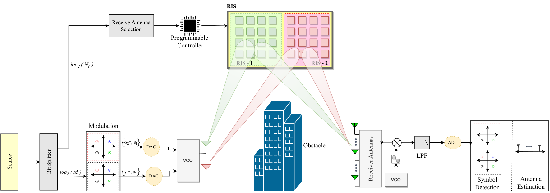
Fig. 1: System model of the RIS-RSM-ASBC scheme.

In this paper, we propose a RIS-based received SM scheme with Alamouti space-time block coding to improve the error performance of conventional RIS-based systems. Also, the theoretical derivations of error performance are presented for the proposed scheme.

I-A Motivation and Contribution

Motivated by the provides ultra-reliable communication, especially at low SNR and achieving better error performance compared to the RIS-RSM [13] in the literature, we investigate the RIS-RSM-ASBC in this paper. Also, we study RIS-RSM-ASBC for the potential data rate improvement using the SM scheme at the receiver side instead of the transmitter. The novel contribution of our paper can be summarized as follows:

  • •

    For the first time in literature, we propose an Alamouti’s coded RIS-assisted SM at the receiver using optimal ML Detector.

  • •

    We represent the theoretical error performance of the proposed scheme and provide useful insights.

  • •

    We compare the error performance of the proposed scheme and other schemes such as conventional RIS-TSM, RIS-TQSM, RIS-RSM, RIS-TSSK-ASBC, and RIS-TSSK-VBLAST.

  • •

    It is aimed to get over 10 dB better error performance in the RIS-RSM-ASBC compared to the RIS-TSSK-ASBC system.

  • •

    Also, another goal is to achieve better error performance with less reflectors in the proposed scheme compared to RIS-RSM.

  • •

    We show that the proposed scheme provides performance enhancement and enables highly reliable transmission, especially at low SNR.

  • •

    Lastly, the simulations and theoretical results are evaluated at low SNR to show the proposed scheme enables highly reliable transmission.

I-B Notations

Matrices and vectors are shown in boldface uppercase and boldface lowercase letter, respectively. (⋅)∗\left(\cdot\right)^{*}, (⋅)T\left(\cdot\right)^{T}, and (⋅)H\left(\cdot\right)^{H} define complex conjugation, transposition, and Hermitian transposition, respectively. [⋅]−1[\cdot]^{-1} and 𝐈n×n\mathbf{I}_{n\times n} stand the inverse of a matrix and the identity matrix with n×nn\times n, respectively. MM defines modulation order. XℜX_{\Re} and XℑX_{\Im} denote the real and imaginary part of XX, respectively. Parameters/symbols used in this paper are also listed in the Table I.

I-C Paper Organization

The remainder of this paper is organized as follows. Section II introduces the principle of the Alamouti’s coded RIS-based Received SM scheme and defines the received signal model. Section III presents the derivation of the proposed system’s BEP. The analytical and Monte Carlo simulation results and complexity analysis are given in Section IV. Finally, Section V concludes the paper.

TABLE I: List of Parameters/Symbols
Parameters/Symbols Definition
E​[X]​(μX)\mathrm{E}\left[X\right](\mu_{X}) Mean of RV X
Var⁡[X]​(σX2)\mathrm{Var}\left[X\right](\sigma^{2}_{X}) Variance of RV X
E⁡[Xn]​(mX⁡(n))\mathrm{E}[X^{n}](m_{X(n)}) nt​hn^{th} moments of RV X
fX​(⋅)f_{X}\left(\cdot\right) Probability density function (PDF) of RV X
MX​(⋅)M_{X}\left(\cdot\right) Moment generating function (MGF) of RV X
Γ⁡(⋅)\Gamma(\cdot) Gamma function
exp⁡(⋅)\exp\left(\cdot\right) Exponential function
det(⋅)\det\left(\cdot\right) Determinant operation
P⁡(⋅)P\left(\cdot\right) Probability of an event.
N0N_{0} Variance of AWGN noise

II System Model

In this section, we present the working principle of the Alamouti space-time coded RIS-based RSM scheme depicted in Fig. 1. In our scheme, we propose the RIS as an access point (AP) that reflects the signals generated by a nearby radio frequency (RF) source thereby, transmission between the source and RIS is not affected by fading. Also, the destination, which consists of the NrN_{r} active receive antennas, lies in the far-field of the RIS, so there is no line of side (LOS) between RF source and destination.

In the considered system model, bits generated from the source are split into two groups which have log2⁡(Nr)\log_{2}(N_{r}) and log2⁡(M)\log_{2}(M) bits, respectively. First log2⁡(Nr)\log_{2}(N_{r}) bits determine the receive antenna index to adjust the RIS phases. The other log2⁡(M)\log_{2}(M) bits are transmitted to the modulation block. After two symbols are selected in the modulation block, these symbols are transmitted to voltage-controlled oscillator (VCO) by digital-to-analog converter (DAC). Signals carried to the IF by VCO reflected in the pre-defined receive antenna using RIS with NN reflector elements. Then, the received signals are brought to the baseband using a mixer and ow pass filter (LPF). The baseband signals are converted into digital signals, which are binary numbers. Lastly, we decide the received symbol and received antenna index according to digital output.

The RIS is equipped with NN passive reflecting elements. In this concept, we divide the RIS into two sub-surfaces, RIS-1 and RIS-2, both of which have N/2N/2 reflector elements. Each full transmission consists of two time slots in which we assume that the wireless fading channel does not change. The wireless fading channel between the receive antenna and it​hi^{th} reflector element in each sub-surface can be represented as below;

hl,i=βl,i×e−j​Θl,il=1,⋯,Nr,h_{l,i}=\beta_{l,i}\times e^{-j\Theta_{l,i}}\quad\quad l=1,\cdots,N_{r}, (1)

where Θl,i\Theta_{l,i} is the channel phase induced by the it​hi^{th} reflector at the lt​hl^{th} receive antenna, and βl,i\beta_{l,i} is the channel fading coefficients followed Rayleigh distribution.

The controller determines the receiver antenna index according to log2⁡Nr\log_{2}N_{r} information bits in the first time slot. Using selected receiver antenna index, the channel phase of both sub-surfaces which are upper and lower are obtained as Θ1=α1\Theta_{1}=\alpha_{1} and Θ2=α2\Theta_{2}=\alpha_{2}, respectively. Then, the RIS reflects the signal s1s_{1} which is loaded into upper sub-surface RIS-1 and s2s_{2} which is loaded into lower sub-surface RIS-2. The base-band signal at lt​hl^{th} receive antenna of the destination in the first time slot can be expressed as:

yl1=s1​∑i=1N/2hl,i​ej​Θm,i+s2​∑i=N2+1Nhl,i​ej​Θm,i+nl1,y^{1}_{l}=s_{1}\sum_{i=1}^{N/2}h_{l,i}e^{j\Theta_{m,i}}+s_{2}\sum_{i=\frac{N}{2}+1}^{N}h_{l,i}e^{j\Theta_{m,i}}+n^{1}_{l}, (2)

where m∈{1,2,…,Nr}m\in\{1,2,\ldots,N_{r}\} and nl1n^{1}_{l} stand for the selected receive antenna and AWGN. The first and second terms come from upper sub-surface and lower sub-surface, respectively. We followed the same methods except transmitted symbols reflected from the RIS in the second time slot. We can represent the base-band signal at the lt​hl^{th} receive antenna in the second time slot as below:

y2l=−s2∗∑i=1N/2hl,iej​Θm,i+s1∗∑i=N2+1Nhl,iej​Θm,i+n2l.y^{2}_{l}=-{s_{2}}^{*}\sum_{i=1}^{N/2}h_{l,i}e^{j\Theta_{m,i}}+{s_{1}}^{*}\sum_{i=\frac{N}{2}+1}^{N}h_{l,i}e^{j\Theta_{m,i}}+n^{2}_{l}. (3)

The spectral efficiency of RIS-RSM-ASBC system is η=(2×log2⁡M+log2⁡Nr)/2\eta=\left(2\times\log_{2}{M}+\log_{2}{N_{r}}\right)/2 bits per channel use (bpcu) wheres traditional SM and RIS-RSM are log2⁡M+log2⁡Nr\log_{2}{M}+\log_{2}{N_{r}}. It is clear that RIS-RSM-ASBC provides better spectral efficiency than classical SM schemes.

After combining (2) and (3) into a matrix form, we get following:

𝐲l\displaystyle\mathbf{y}_{l} =[yl1yl2]T=\displaystyle=\left[y^{1}_{l}\quad y^{2}_{l}\right]^{T}= (4)
[s1s2−s2∗s1∗]⏟𝐒​[∑i=1N/2βl,i​e−j​Θl,i​ej​Θm,i∑i=1+N/2Nβl,i​e−j​Θl,i​ej​Θm,i]⏟𝐡l+[nl1nl2]⏟𝐧l.\displaystyle\underbrace{\left[\begin{array}[]{cc}s_{1}&s_{2}\\ -s_{2}^{*}&s_{1}^{*}\end{array}\right]}_{\mathbf{S}}\underbrace{\left[\begin{array}[]{c}\sum_{i=1}^{N/2}\beta_{l,i}e^{-j\Theta_{l,i}}e^{j\Theta_{m},i}\\ \sum_{i=1+N/2}^{N}\beta_{l,i}e^{-j\Theta_{l,i}}e^{j\Theta_{m},i}\end{array}\right]}_{\mathbf{h}_{l}}+\underbrace{\left[\begin{array}[]{c}{n}_{l}^{1}\\ {n}_{l}^{2}\end{array}\right]}_{\mathbf{n}_{l}}.

At the receiver ML detector is utilized. We have applying ML into (4) to recover transmitted symbols and receiver antenna index:

(s^1,s^2,m^)=arg⁡min⁡∑l=1Nrs1,s2,m⁡‖𝐲l−𝐒𝐡l‖2,\Big(\hat{s}_{1},\hat{s}_{2},\hat{m}\Big)=\arg\min\limits_{s_{1},s_{2},m}\sum\limits_{l=1}^{N_{r}}{\Big|\Big|\mathbf{y}_{l}-\mathbf{S}\mathbf{h}_{l}\Big|\Big|^{2}}, (5)

where s^1\hat{s}_{1}, s^2\hat{s}_{2}, m^\hat{m} are estimation of s1{s}_{1}, s2{s}_{2}, m{m} respectively.

III Performance Analysis

In this section, theoretical average bit error rate (ABER) expression of the Alamouti coded RIS-based SM scheme are provided by evaluating pairwise error probability (PEP) and utilizing optimal ML detector.

The conditional PEP expression of proposed system can be expressed as following:

P(m,𝐒→m^,𝐒^|𝐡)\displaystyle P\left(m,\mathbf{S}\rightarrow\hat{m},\hat{\mathbf{S}}\big|\mathbf{h}\right) (6)
=\displaystyle\!\!\!\!\!\!\!\!\!\!\!\!\!\!\!\!\!\!\!\!\!\!\!\!\!\!\!\!\!\!\!\!\!\!\!\!\!\!\!\!\!\!\!\!\!\!\!\!\!\!\!\!\!\!\!\!\!\!\!\!\!\!\!\!\!\!\!\!\!\!\!\!= P⁡(∑l=1Nr‖𝐲l−𝐒𝐡l‖2<∑l=1Nr‖𝐲l^−𝐒^​𝐡l^‖2).\displaystyle\!\!\!\!\!\!\!\!\!\!\!\!\!\!\!\!\!\!\!\!\!\!\!\!\!\!\!\!\!\!\!\!\!\!\!\!\!P\left(\sum_{l=1}^{N_{r}}\Big|\Big|\mathbf{y}_{l}-\mathbf{S}\mathbf{h}_{l}\Big|\Big|^{2}<\sum_{l=1}^{N_{r}}\Big|\Big|\mathbf{y}_{\hat{l}}-\mathbf{\hat{S}}\mathbf{h}_{\hat{l}}\Big|\Big|^{2}\right)\!.

Re-arranging (6) gives us the following:

P(m,𝐒→m^,𝐒^|𝐡)\displaystyle P\left(m,\mathbf{S}\rightarrow\hat{m},\hat{\mathbf{S}}\big|\mathbf{h}\right)
=\displaystyle\!\!\!\!\!\!\!\!\!\!\!\!\!\!\!\!\!\!\!\!\!\!\!\!\!\!\!\!\!\!\!\!\!\!\!\!\!\!\!\!\!\!\!\!\!\!\!\!\!\!\!\!\!\!\!\!\!\!\!\!\!\!\!\!\!\!\!\!\!\!\!\!\!\!\!\!\!\!\!\!\!\!\!\!\!\!\!\!\!\!\!\!\!\!\!\!\!\!\!\!\!\!\!\!\!\!\!\!= P⁡(∑l=1Nr‖𝐧l‖2>∑l=1Nr‖𝐒𝐡l+𝐧l^−𝐒^​𝐡l^‖2)\displaystyle\!\!\!\!\!\!\!\!\!\!\!\!\!\!\!\!\!\!\!\!\!\!\!\!\!\!\!\!\!\!\!\!\!\!\!\!\!\!\!\!\!\!\!\!\!\!\!\!\!\!\!\!\!\!\!\!\!P\left(\sum_{l=1}^{N_{r}}\Big|\Big|\mathbf{n}_{l}\Big|\Big|^{2}>\sum_{l=1}^{N_{r}}\Big|\Big|\mathbf{S}\mathbf{h}_{l}+\mathbf{n}_{\hat{l}}-\mathbf{\hat{S}}\mathbf{h}_{\hat{l}}\Big|\Big|^{2}\right)
=\displaystyle\!\!\!\!\!\!\!\!\!\!\!\!\!\!\!\!\!\!\!\!\!\!\!\!\!\!\!\!\!\!\!\!\!\!\!\!\!\!\!\!\!\!\!\!\!\!\!\!\!\!\!\!\!\!\!\!\!\!\!\!\!\!\!\!\!\!\!\!\!\!\!\!\!\!\!\!\!\!\!\!\!\!\!\!\!\!\!\!\!\!\!\!\!\!\!\!\!\!\!\!\!\!\!\!\!\!\!\!= P⁡(∑l=1Nr‖𝐧l‖2−(𝐒𝐡l−𝐒^​𝐡l^+𝐧l)CLOSE\displaystyle\!\!\!\!\!\!\!\!\!\!\!\!\!\!\!\!\!\!\!\!\!\!\!\!\!\!\!\!\!\!\!\!\!\!\!\!\!\!\!\!\!\!\!\!\!\!\!\!\!\!\!\!\!\!\!\!\!P\left(\sum_{l=1}^{N_{r}}\Big|\Big|\mathbf{n}_{l}\Big|\Big|^{2}-\left(\mathbf{S}\mathbf{h}_{l}-\mathbf{\hat{S}}\mathbf{h}_{\hat{l}}+\mathbf{n}_{l}\right)\right.
×\displaystyle\!\!\!\!\!\!\!\!\!\!\!\!\!\!\!\!\!\!\!\!\!\!\!\!\!\!\!\!\!\!\!\!\!\!\!\!\!\!\!\!\!\!\!\!\!\!\!\!\!\!\!\!\!\!\!\!\!\!\!\!\!\!\!\!\!\!\!\!\!\!\!\!\!\!\!\!\!\!\!\!\!\!\!\!\!\!\!\!\!\!\!\!\!\!\!\!\!\!\!\!\!\!\!\!\!\!\!\!\times OPEN(𝐒𝐡l−𝐒^​𝐡l^+𝐧l^)H>0)\displaystyle\!\!\!\!\!\!\!\!\!\!\!\!\!\!\!\!\!\!\!\!\!\!\!\!\!\!\!\!\!\!\!\!\!\!\!\!\!\!\!\!\!\!\!\!\!\!\!\!\!\!\!\!\!\!\!\!\!\left.\left(\mathbf{S}\mathbf{h}_{l}-\mathbf{\hat{S}}\mathbf{h}_{\hat{l}}+\mathbf{n}_{\hat{l}}\right)^{H}>0\right)
=\displaystyle\!\!\!\!\!\!\!\!\!\!\!\!\!\!\!\!\!\!\!\!\!\!\!\!\!\!\!\!\!\!\!\!\!\!\!\!\!\!\!\!\!\!\!\!\!\!\!\!\!\!\!\!\!\!\!\!\!\!\!\!\!\!\!\!\!\!\!\!\!\!\!\!\!\!\!\!\!\!\!\!\!\!\!\!\!\!\!\!\!\!\!\!\!\!\!\!\!\!\!\!\!\!\!\!\!\!\!\!= P⁡(∑l=1Nr−||𝐒𝐡l−𝐒^𝐡l^||2−2ℜ(𝐧l^H(𝐒𝐡l−𝐒^𝐡l^))⏟𝒦>0)\displaystyle\!\!\!\!\!\!\!\!\!\!\!\!\!\!\!\!\!\!\!\!\!\!\!\!\!\!\!\!\!\!\!\!\!\!\!\!\!\!\!\!\!\!\!\!\!\!\!\!\!\!\!\!\!\!\!\!\!P\Bigg(\underbrace{\sum_{l=1}^{N_{r}}-\Big|\Big|\mathbf{S}\mathbf{h}_{l}-\hat{\mathbf{S}}\mathbf{h}_{\hat{l}}\Big|\Big|^{2}-2\Re\left(\mathbf{n}_{\hat{l}}^{H}\left(\mathbf{S}\mathbf{h}_{l}-\mathbf{\hat{S}}\mathbf{h}_{\hat{l}}\right)\right)}_{\mathcal{K}}>0\Bigg)

where 𝒦\mathcal{K} is Gaussian R.V with mean μ𝒦=−∑l=1Nr||𝐒𝐡l−𝐒^𝐡l^||2\mu_{\mathcal{K}}=-\sum_{l=1}^{N_{r}}\big|\big|\mathbf{S}\mathbf{h}_{l}-\hat{\mathbf{S}}\mathbf{h}_{\hat{l}}\big|\big|^{2} and variance σ𝒦2=∑l=1Nr2​No​‖𝐒𝐡l−𝐒^​𝐡l^‖2\sigma^{2}_{\mathcal{K}}=\sum_{l=1}^{N_{r}}2N_{o}\big|\big|\mathbf{S}\mathbf{h}_{l}-\hat{\mathbf{S}}\mathbf{h}_{\hat{l}}\big|\big|^{2}.

As known, QQ function can be defined as [19]:

P⁡(X>x)=Q⁡(x)=12​π​∫x∞exp⁡(−u22)​𝑑u,P\left(X>x\right)=Q\left(x\right)=\frac{1}{2\pi}\int_{x}^{\infty}\exp\left({\frac{-u^{2}}{2}}\right)du, (8)

where X∼𝒩⁡(0,1)X\sim\mathcal{N}\left(0,1\right). So when we go back to our equation (), statistical values of 𝒦\mathcal{K} is re-arranged doing by normalization of the its standard deviation and shifting its mean to zero. Therefore the following expression is obtained:

P(m,𝐒→m^,𝐒^|𝐡)\displaystyle P\left(m,\mathbf{S}\rightarrow\hat{m},\hat{\mathbf{S}}\Big|\mathbf{h}\right) =Q⁡(−μ𝒦σ𝒦)\displaystyle=Q\left(\frac{-\mu_{\mathcal{K}}}{\sigma_{\mathcal{K}}}\right) (9)
=Q⁡(∑l=1Nr‖𝐒𝐡l−𝐒^​𝐡l^‖22​N0).\displaystyle=Q\left(\sqrt{\frac{\sum_{l=1}^{N_{r}}\Big|\Big|\mathbf{S}\mathbf{h}_{l}-\hat{\mathbf{S}}\mathbf{h}_{\hat{l}}\Big|\Big|^{2}}{2N_{0}}}\right).

Afterwards, the unconditional PEP expression can be obtained taking by the expectation of (6):

P¯e(m,𝐒→m^,𝐒^)=∫0∞Q(Γ2​N0)fΓ(Γ)=1π​∫0∞∫0π/2exp⁡(−Γ4​sin2⁡Θ​N0)​fΓ​(Γ)​𝑑Θ​𝑑ΓP¯e(m,𝐒→m^,𝐒^)=1π∫0π/2MΓ(−14​sin2⁡Θ​N0),\overline{P}_{e}\left(m,\mathbf{S}\rightarrow\hat{m},\hat{\mathbf{S}}\right)=\int_{0}^{\infty}Q\left(\sqrt{\frac{\Gamma}{2N_{0}}}\right)f_{\Gamma}(\Gamma)\\ =\frac{1}{\pi}\int_{0}^{\infty}\int_{0}^{\pi/2}\exp{\left(-\frac{\Gamma}{4\sin^{2}{\Theta}N_{0}}\right)f_{\Gamma}\left(\Gamma\right)d\Theta d\Gamma}\\ \overline{P}_{e}\left(m,\mathbf{S}\rightarrow\hat{m},\hat{\mathbf{S}}\right)=\frac{1}{\pi}\int_{0}^{\pi/2}M_{\Gamma}\left(-\frac{1}{4\sin^{2}{\Theta}N_{0}}\right), (10)

where Γ=∑l=1Nr‖𝐒𝐡l−𝐒^​𝐡l^‖2\Gamma=\sum_{l=1}^{N_{r}}\Big|\Big|\mathbf{S}\mathbf{h}_{l}-\hat{\mathbf{S}}\mathbf{h}_{\hat{l}}\Big|\Big|^{2}.

We need the MGF of Γ\Gamma (MΓ​(s))(M_{\Gamma}(s)) to perform this integration. So we will divide the R.V Γ\Gamma into two parts. From this point of view, we can re-write the Γ\Gamma more precisely as follows:

Γ=ΓT​s1+ΓT​s2,\Gamma=\Gamma_{Ts_{1}}+\Gamma_{Ts_{2}}, (11)

where

ΓT​s1\displaystyle\Gamma_{Ts_{1}} =∑l=1N​r|∑i=1N/2βl,ie−j​Θl,i(ej​Θm,is1−ej​Θm^,is^1)\displaystyle=\sum_{l=1}^{Nr}\left|\sum_{i=1}^{N/2}\beta_{l,i}e^{-j\Theta_{l,i}}\left(e^{j\Theta_{m,i}}s_{1}-e^{j\Theta_{\hat{m},i}}\hat{s}_{1}\right)\right. (12)
+∑i=1+N/2Nβl,ie−j​Θl,i(ej​Θm,is2−ej​Θm^,is^2)|2,\displaystyle+\left.\sum_{i=1+N/2}^{N}\beta_{l,i}e^{-j\Theta_{l,i}}\left(e^{j\Theta_{m,i}}s_{2}-e^{j\Theta_{\hat{m},i}}\hat{s}_{2}\right)\right|^{2},
ΓT​s2\displaystyle\Gamma_{Ts_{2}} =∑l=1N​r|−∑i=1N/2βl,ie−j​Θl,i(ej​Θm,is2∗−ej​Θm^,is^2∗)\displaystyle=\sum_{l=1}^{Nr}\left|-\sum_{i=1}^{N/2}\beta_{l,i}e^{-j\Theta_{l,i}}\left(e^{j\Theta_{m,i}}s_{2}^{*}-e^{j\Theta_{\hat{m},i}}\hat{s}_{2}^{*}\right)\right.
+∑i=1+N/2Nβl,ie−j​Θl,i(ej​Θm,is1∗−ej​Θm^,is^1∗)|2.\displaystyle+\left.\sum_{i=1+N/2}^{N}\beta_{l,i}e^{-j\Theta_{l,i}}\left(e^{j\Theta_{m,i}}s_{1}^{*}-e^{j\Theta_{\hat{m},i}}\hat{s}_{1}^{*}\right)\right|^{2}.

The point to be noted in this expression is the fact that the ΓT​s1\Gamma_{Ts_{1}} and ΓT​s2\Gamma_{Ts_{2}} are independent of each other due to the fact that signals are experienced with different time zones. Plus, ΓT​s1 =Δ Γ1\Gamma_{Ts_{1}}\mathrel{\hbox{\hskip 3.8889pt\hskip-3.8889pt\hbox{$=$}\hskip-3.8889pt\hskip-3.28473pt\raisebox{4.66875pt}{\hbox{$\scriptstyle\Delta$}}\hskip-3.28473pt\hskip 3.8889pt}}\Gamma_{1} and ΓT​s2 =Δ Γ2\Gamma_{Ts_{2}}\mathrel{\hbox{\hskip 3.8889pt\hskip-3.8889pt\hbox{$=$}\hskip-3.8889pt\hskip-3.28473pt\raisebox{4.66875pt}{\hbox{$\scriptstyle\Delta$}}\hskip-3.28473pt\hskip 3.8889pt}}\Gamma_{2} will be expressed as for the simplicity. Therefore, separate MGF derivations will be made for two time slots.

III-A The MGFs Derivation for First Time Slot

This MGF can be derived by considering the general quadratic form of correlated Gaussian RVs and depends on erroneous or correct detection of the receive antenna index mm.

III-A1 Under the wrong antenna decision, m≠m^m\neq\hat{m}

TABLE II: The expressions of Γ11,Γ12,Γ13,Γ21\Gamma_{11},\Gamma_{12},\Gamma_{13},\Gamma_{21}, Γ22\Gamma_{22} and Γ23\Gamma_{23} (First row: Time Slot-1 and Second row: Time Slot-2).
Γ11=|∑i=1N/2βm,i​(s1−e−j​Ψi​s^1)+∑i=1+N/2Nβm,i​(s2−e−j​Ψi​s^2)|2Γ12=|∑i=1N/2βm^,i​(s1​e−j​Ψi−s^1)+∑i=1+N/2Nβm^,i​(s2​e−j​Ψi−s^2)|2Γ13=∑l=1​(l≠m,l≠m^)Nr|∑i=1N/2βl,i(s1e−j​Θl,i−s^1e−j​Θm^,i)+∑i=1+N/2Nβl,i(s2e−j​Θl,i−s^2e−j​Θm^,i)|2\begin{aligned} \Gamma_{11}&=\left|\sum_{i=1}^{N/2}\beta_{m,i}\left(s_{1}-e^{-j\Psi_{i}}\hat{s}_{1}\right)+\!\!\!\!\!\!\!\sum_{i=1+N/2}^{N}\!\!\!\!\!\beta_{m,i}\left(s_{2}-e^{-j\Psi_{i}}\hat{s}_{2}\right)\right|^{2}\\ \Gamma_{12}&=\left|\sum_{i=1}^{N/2}\beta_{\hat{m},i}\left(s_{1}e^{-j\Psi_{i}}-\hat{s}_{1}\right)+\!\!\!\!\!\!\!\sum_{i=1+N/2}^{N}\!\!\!\!\!\beta_{\hat{m},i}\left(s_{2}e^{-j\Psi_{i}}-\hat{s}_{2}\right)\right|^{2}\\ \Gamma_{13}&=\sum_{l=1(l\neq m,l\neq\hat{m})}^{N_{r}}\Bigg|\sum_{i=1}^{N/2}\beta_{l,i}\left(s_{1}e^{-j\Theta_{l,i}}-\hat{s}_{1}e^{-j\Theta_{\hat{m},i}}\right)\\ &+\sum_{i=1+N/2}^{N}\beta_{l,i}\left(s_{2}e^{-j\Theta_{l,i}}-\hat{s}_{2}e^{-j\Theta_{\hat{m},i}}\right)\Bigg|^{2}\end{aligned}
Γ21=|∑i=1N/2βm,i​(−s2∗+e−j​Ψi​s^2∗)+∑i=1+N/2Nβm,i​(s1∗−e−j​Ψi​s^1∗)|2Γ22=|∑i=1N/2βm^,i​(s^2∗−s2∗​e−j​Ψi)+∑i=1+N/2Nβm^,i​(s1∗​e−j​Ψi−s^1∗)|2Γ23=∑l=1​(l≠m,l≠m^)Nr|∑i=1N/2βl,i(s1∗e−j​Θm,i−s^1∗e−j​Θm^,i)+∑i=1+N/2Nβl,i(s2∗e−j​Θm,i−s^2∗e−j​Θm^,i)|2\begin{aligned} \\ \Gamma_{21}&=\left|\sum_{i=1}^{N/2}\beta_{m,i}\left(-s_{2}^{*}+e^{-j\Psi_{i}}\hat{s}_{2}^{*}\right)+\!\!\!\!\!\!\!\sum_{i=1+N/2}^{N}\!\!\!\!\!\beta_{m,i}\left(s_{1}^{*}-e^{-j\Psi_{i}}\hat{s}_{1}^{*}\right)\right|^{2}\\ \Gamma_{22}&=\left|\sum_{i=1}^{N/2}\beta_{\hat{m},i}\left(\hat{s}^{*}_{2}-s_{2}^{*}e^{-j\Psi_{i}}\right)+\!\!\!\!\!\!\!\sum_{i=1+N/2}^{N}\!\!\!\!\!\beta_{\hat{m},i}\left(s_{1}^{*}e^{-j\Psi_{i}}-\hat{s}_{1}^{*}\right)\right|^{2}\\ \Gamma_{23}&=\sum_{l=1(l\neq m,l\neq\hat{m})}^{N_{r}}\Bigg|\sum_{i=1}^{N/2}\beta_{l,i}\left(s_{1}^{*}e^{-j\Theta_{m,i}}-\hat{s}_{1}^{*}e^{-j\Theta_{\hat{m},i}}\right)\\ &+\sum_{i=1+N/2}^{N}\beta_{l,i}\left(s_{2}^{*}e^{-j\Theta_{m,i}}-\hat{s}_{2}^{*}e^{-j\Theta_{\hat{m},i}}\right)\Bigg|^{2}\end{aligned}

We can re-write Γ1\Gamma_{1} as Γ1=Γ11+Γ12+Γ13\Gamma_{1}=\Gamma_{11}+\Gamma_{12}+\Gamma_{13} and these R.Vs are defined in Table II. In this manner, Γ11\Gamma_{11}, Γ12\Gamma_{12} and Γ13\Gamma_{13} stand for l=ml=m, l=m^l=\hat{m} and l≠m^,l≠ml\neq\hat{m},l\neq m. Also, Ψi=Θm,i−Θm^,i\Psi_{i}=\Theta_{m,i}-\Theta_{\hat{m},i} is with having triangular distribution [20]:

fΨ​(x)={2​π​(1+x2​π);−2​π<x<02​π​(1−x2​π);0<x<2​πf_{\Psi}(x)=\left\{\begin{array}[]{rcl}{2\pi}\left(1+\frac{x}{2\pi}\right);&-2\pi<x<0\\ {2\pi}\left(1-\frac{x}{2\pi}\right);&0<x<2\pi\end{array}\right. (13)

Here, we will firstly derive the MGF expression of Γ11+Γ12\Gamma_{11}+\Gamma_{12}. After that, MGF of Γ13\Gamma_{13} will be presented. It is known that the MGF of the sum of two independent R.Vs is equal to the product of their MGFs. Hence, we will obtain MGF of Γ1\Gamma_{1} as MΓ1=M(Γ11+Γ12)×MΓ13M_{\Gamma_{1}}=M_{\left(\Gamma_{11}+\Gamma_{12}\right)}\times M_{\Gamma_{13}}.

TABLE III: The derivation of entities of 𝐦\mathbf{m} and 𝐦~\mathbf{\tilde{\mathbf{m}}}, (First row: Time Slot-1 and Second row: Time Slot-2)
μ(Δ11)ℜ=N​π4​((s1)ℜ+(s2)ℜ),μ(Δ11)ℑ=N​π4​((s1)ℑ+(s2)ℑ),μ(Δ12)ℜ=−N​π4​((s^1)ℜ+(s^2)ℜ)μ(Δ12)ℑ=−N​π4​((s^1)ℜ+(s^2)ℜ)μ(Δ21)ℜ=N​π4​((s1∗)ℜ−(s2∗)ℜ)μ(Δ21)ℑ=N​π4​((s1∗)ℑ−(s2∗)ℑ),μ(Δ22)ℜ=−N​π4​((s^1∗)ℜ−(s^2∗)ℜ)μ(Δ22)ℑ=−N​π4​((s^1∗)ℜ−(s^2∗)ℜ)\begin{aligned} \mu_{\left(\Delta_{11}\right)_{\Re}}&=\frac{N\sqrt{\pi}}{4}\Big((s_{1})_{\Re}+(s_{2})_{\Re}\Big),\\ \mu_{\left(\Delta_{11}\right)_{\Im}}&=\frac{N\sqrt{\pi}}{4}\Big((s_{1})_{\Im}+(s_{2})_{\Im}\Big),\\ \mu_{\left(\Delta_{12}\right)_{\Re}}&=-\frac{N\sqrt{\pi}}{4}\Big(\left(\hat{s}_{1}\right)_{\Re}+(\hat{s}_{2})_{\Re}\Big)\par\\ \mu_{\left(\Delta_{12}\right)_{\Im}}&=-\frac{N\sqrt{\pi}}{4}\Big((\hat{s}_{1})_{\Re}+(\hat{s}_{2})_{\Re}\Big)\\ \\ \hline\cr\\ \mu_{\left(\Delta_{21}\right)_{\Re}}&=\frac{N\sqrt{\pi}}{4}\Big((s^{*}_{1})_{\Re}-(s^{*}_{2})_{\Re}\Big)\\ \mu_{\left(\Delta_{21}\right)_{\Im}}&=\frac{N\sqrt{\pi}}{4}\Big((s^{*}_{1})_{\Im}-(s^{*}_{2})_{\Im}\Big),\\ \mu_{\left(\Delta_{22}\right)_{\Re}}&=-\frac{N\sqrt{\pi}}{4}\Big(\left(\hat{s}^{*}_{1}\right)_{\Re}-(\hat{s}^{*}_{2})_{\Re}\Big)\\ \mu_{\left(\Delta_{22}\right)_{\Im}}&=-\frac{N\sqrt{\pi}}{4}\Big((\hat{s}^{*}_{1})_{\Re}-(\hat{s}^{*}_{2})_{\Re}\Big)\end{aligned}

Keeping in mind, Γ11=|Δ11|2=(Δ11)ℜ2+(Δ11)ℑ2\Gamma_{11}=|\Delta_{11}|^{2}=\left({\Delta_{11}}\right)^{2}_{\Re}+\left({\Delta_{11}}\right)^{2}_{\Im} , Γ12=|Δ12|2=(Δ12)ℜ2+(Δ12)ℑ2\Gamma_{12}=|\Delta_{12}|^{2}=\left({\Delta_{12}}\right)^{2}_{\Re}+\left({\Delta_{12}}\right)^{2}_{\Im} and Γ11+Γ12=𝐱T​𝐀𝐱\Gamma_{11}+\Gamma_{12}=\mathbf{x}^{T}\mathbf{A}\mathbf{x} where

𝐱\displaystyle\mathbf{x} =[(Γ11)ℜ(Γ11)ℑ(Γ12)ℜ(Γ12)ℑ]T,\displaystyle=\Big[\begin{array}[]{cccc}\left(\Gamma_{11}\right)_{\Re}&\left(\Gamma_{11}\right)_{\Im}&\left(\Gamma_{12}\right)_{\Re}&\left(\Gamma_{12}\right)_{\Im}\end{array}\Big]^{T}, (14)
𝐀\displaystyle\mathbf{A} =[1000010000100001]\displaystyle=\begin{bmatrix}1&0&0&0\\ 0&1&0&0\\ 0&0&1&0\\ 0&0&0&1\end{bmatrix}
𝐱T​𝐀𝐱\displaystyle\mathbf{x}^{T}\mathbf{A}\mathbf{x} =(Δ11)ℜ2+(Δ11)ℑ2+(Δ12)ℜ2+(Δ12)ℑ2\displaystyle=\left({\Delta_{11}}\right)^{2}_{\Re}+\left({\Delta_{11}}\right)^{2}_{\Im}+\left({\Delta_{12}}\right)^{2}_{\Re}+\left({\Delta_{12}}\right)^{2}_{\Im}

Let 𝒢=Γ11+Γ12\mathcal{G}=\Gamma_{11}+\Gamma_{12}, then MGF of 𝒢\mathcal{G} can be obtained as follows [21, Eq. (3.2a.1)]:

M𝒢​(s)\displaystyle M_{\mathcal{G}}(s) =(det​(𝐈−2​s​𝐀𝐂))−1\displaystyle=\left(\sqrt{\textrm{det}\left(\mathbf{I}-2s\mathbf{AC}\right)}\right)^{-1} (15)
×exp⁡(−12​𝐦T​[𝐈−(𝐈−2​s​𝐀𝐂)−1]​𝐂−1).\displaystyle\times\exp\left(-\frac{1}{2}\mathbf{m}^{T}\left[\mathbf{I}-\left(\mathbf{I}-2s\mathbf{AC}\right)^{-1}\right]\mathbf{C}^{-1}\right).

where 𝐦\mathbf{m} and 𝐂\mathbf{C} are the mean vector and the covariance matrix of 𝐱\mathbf{x}, respectively. We can define mean vector of 𝐱\mathbf{x} by 𝐦=[μ(Δ11)ℜμ(Δ11)ℑμ(Δ12)ℜμ(Δ12)ℑ]T\mathbf{m}=\left[\begin{array}[]{cccc}\mu_{\left(\Delta_{11}\right)_{\Re}}&\mu_{\left(\Delta_{11}\right)_{\Im}}&\mu_{\left(\Delta_{12}\right)_{\Re}}&\mu_{\left(\Delta_{12}\right)_{\Im}}\end{array}\right]^{T}. The entities of 𝐦\mathbf{m} can be represented in Table III.

TABLE IV: Statistical Properties of the covariance entities of 𝐂\mathbf{C} and 𝐂~\tilde{\mathbf{C}} (First row: Time Slot-1 and Second row: Time Slot-2)
σ12=N8​(4−π)​((s1)ℜ2+(s2)ℜ2)+N4​(|s^1|2+|s^2|2),σ1,3=−N​π16​((s1)ℜ​(s^1)ℜ+(s1)ℑ​(s^1)ℑ+(s2)ℜ​(s^2)ℜ+(s2)ℑ​(s^2)ℑ)σ22=N8​(4−π)​((s1)ℑ2+(s2)ℑ2)+N4​(|s^1|2+|s^2|2),σ1,4=−N​π16​((s1)ℑ​(s^1)ℜ+(s1)ℜ​(s^1)ℑ+(s2)ℑ​(s^2)ℜ+(s2)ℜ​(s^2)ℑ)σ32=N8​(4−π)​((s^1)ℜ2+(s^2)ℜ2)+N4​(|s1|2+|s2|2),σ2,4=N​π16​((s1)ℜ​(s^1)ℜ+(s1)ℑ​(s^1)ℑ+(s2)ℜ​(s^2)ℜ+(s2)ℑ​(s^2)ℑ)σ42=N8​(4−π)​((s1)ℑ2+(s2)ℑ2)+N4​(|s1|2+|s2|2),σ2,3=−N​π16​((s^1)ℜ​(s1)ℑ+(s1)ℜ​(s^1)ℑ+(s2)ℑ​(s^2)ℜ+(s2)ℜ​(s^2)ℑ)σ1,2=N⁡(4−π)8​((s1)ℜ​(s1)ℑ+(s2)ℜ​(s2)ℑ),σ3,4=N⁡(4−π)8​((s^1)ℜ​(s^1)ℑ+(s^2)ℜ​(s^2)ℑ)\begin{aligned} \sigma_{1}^{2}&=\frac{N}{8}\left(4-\pi\right)\Big((s_{1})_{\Re}^{2}+(s_{2})_{\Re}^{2}\Big)+\frac{N}{4}\Big(|\hat{s}_{1}|^{2}+|\hat{s}_{2}|^{2}\Big),\;\sigma_{1,3}=\frac{-N\pi}{16}\Big((s_{1})_{\Re}(\hat{s}_{1})_{\Re}+(s_{1})_{\Im}(\hat{s}_{1})_{\Im}+(s_{2})_{\Re}(\hat{s}_{2})_{\Re}+(s_{2})_{\Im}(\hat{s}_{2})_{\Im}\Big)\\ \sigma_{2}^{2}&=\frac{N}{8}\left(4-\pi\right)\Big((s_{1})_{\Im}^{2}+(s_{2})_{\Im}^{2}\Big)+\frac{N}{4}\Big(|\hat{s}_{1}|^{2}+|\hat{s}_{2}|^{2}\Big),\;\sigma_{1,4}=\frac{-N\pi}{16}\Big((s_{1})_{\Im}(\hat{s}_{1})_{\Re}+(s_{1})_{\Re}(\hat{s}_{1})_{\Im}+(s_{2})_{\Im}(\hat{s}_{2})_{\Re}+(s_{2})_{\Re}(\hat{s}_{2})_{\Im}\Big)\\ \sigma_{3}^{2}&=\frac{N}{8}\left(4-\pi\right)\Big((\hat{s}_{1})_{\Re}^{2}+(\hat{s}_{2})_{\Re}^{2}\Big)+\frac{N}{4}\Big(|{s}_{1}|^{2}+|{s}_{2}|^{2}\Big),\;\sigma_{2,4}=\frac{N\pi}{16}\Big((s_{1})_{\Re}(\hat{s}_{1})_{\Re}+(s_{1})_{\Im}(\hat{s}_{1})_{\Im}+(s_{2})_{\Re}(\hat{s}_{2})_{\Re}+(s_{2})_{\Im}(\hat{s}_{2})_{\Im}\Big)\\ \sigma_{4}^{2}&=\frac{N}{8}\left(4-\pi\right)\Big((s_{1})_{\Im}^{2}+(s_{2})_{\Im}^{2}\Big)+\frac{N}{4}\Big(|{s}_{1}|^{2}+|{s}_{2}|^{2}\Big),\;\sigma_{2,3}=\frac{-N\pi}{16}\Big((\hat{s}_{1})_{\Re}(s_{1})_{\Im}+(s_{1})_{\Re}(\hat{s}_{1})_{\Im}+(s_{2})_{\Im}(\hat{s}_{2})_{\Re}+(s_{2})_{\Re}(\hat{s}_{2})_{\Im}\Big)\\ \sigma_{1,2}&=\frac{N(4-\pi)}{8}\Big((s_{1})_{\Re}(s_{1})_{\Im}+(s_{2})_{\Re}(s_{2})_{\Im}\Big),\;\;\;\;\;\;\;\;\;\;\;\;\;\;\;\;\sigma_{3,4}=\frac{N(4-\pi)}{8}\Big((\hat{s}_{1})_{\Re}(\hat{s}_{1})_{\Im}+(\hat{s}_{2})_{\Re}(\hat{s}_{2})_{\Im}\Big)\\ \end{aligned}
σ12=N8​(4−π)​((s1∗)ℜ2+(s2∗)ℜ2)+N4​(|s^1∗|2+|s^2∗|2),σ1,3=N​π16​((s1∗)ℑ​(s^1∗)ℑ−(s1∗)ℜ​(s^1∗)ℜ−(s2∗)ℜ​(s^2∗)ℜ+(s2∗)ℑ​(s^2∗)ℑ)σ22=N8​(4−π)​((s1∗)ℑ2+(s2∗)ℑ2)+N4​(|s^1∗|2+|s^2∗|2),σ1,4=−N​π16​((s1∗)ℑ​(s^1∗)ℜ+(s1∗)ℜ​(s^1∗)ℑ+(s2∗)ℑ​(s^2∗)ℜ+(s2∗)ℜ​(s^2∗)ℑ)σ32=N8​(4−π)​((s^1∗)ℜ2+(s^2∗)ℜ2)+N4​(|s1∗|2+|s2∗|2),σ2,4=N​π16​((s1∗)ℜ​(s^1∗)ℜ−(s1∗)ℑ​(s^1∗)ℑ+(s2∗)ℜ​(s^2∗)ℜ−(s2∗)ℑ​(s^2∗)ℑ)σ42=N8​(4−π)​((s1∗)ℑ2+(s2∗)ℑ2)+N4​(|s1∗|2+|s2∗|2),σ2,3=−N​π16​((s^1∗)ℜ​(s1∗)ℑ+(s1∗)ℜ​(s^1∗)ℑ+(s2∗)ℑ​(s^2∗)ℜ+(s2∗)ℜ​(s^2∗)ℑ)σ1,2=N⁡(4−π)8​((s1∗)ℜ​(s1∗)ℑ+(s2∗)ℜ​(s2∗)ℑ),σ3,4=N⁡(4−π)8​((s^1∗)ℜ​(s^1∗)ℑ+(s^2∗)ℜ​(s^2∗)ℑ)\begin{aligned} \sigma_{1}^{2}&=\frac{N}{8}\left(4-\pi\right)\Big((s^{*}_{1})_{\Re}^{2}+(s^{*}_{2})_{\Re}^{2}\Big)+\frac{N}{4}\Big(|\hat{s}^{*}_{1}|^{2}+|\hat{s}^{*}_{2}|^{2}\Big),\;\sigma_{1,3}=\frac{N\pi}{16}\Big((s^{*}_{1})_{\Im}(\hat{s}^{*}_{1})_{\Im}-(s^{*}_{1})_{\Re}(\hat{s}^{*}_{1})_{\Re}-(s^{*}_{2})_{\Re}(\hat{s}^{*}_{2})_{\Re}+(s^{*}_{2})_{\Im}(\hat{s}^{*}_{2})_{\Im}\Big)\\ \sigma_{2}^{2}&=\frac{N}{8}\left(4-\pi\right)\Big((s^{*}_{1})_{\Im}^{2}+(s^{*}_{2})_{\Im}^{2}\Big)+\frac{N}{4}\Big(|\hat{s}^{*}_{1}|^{2}+|\hat{s}^{*}_{2}|^{2}\Big),\;\sigma_{1,4}=\frac{-N\pi}{16}\Big((s^{*}_{1})_{\Im}(\hat{s}^{*}_{1})_{\Re}+(s^{*}_{1})_{\Re}(\hat{s}^{*}_{1})_{\Im}+(s^{*}_{2})_{\Im}(\hat{s}^{*}_{2})_{\Re}+(s^{*}_{2})_{\Re}(\hat{s}^{*}_{2})_{\Im}\Big)\\ \sigma_{3}^{2}&=\frac{N}{8}\left(4-\pi\right)\Big((\hat{s}^{*}_{1})_{\Re}^{2}+(\hat{s}^{*}_{2})_{\Re}^{2}\Big)+\frac{N}{4}\Big(|{s}^{*}_{1}|^{2}+|{s}^{*}_{2}|^{2}\Big),\;\sigma_{2,4}=\frac{N\pi}{16}\Big((s^{*}_{1})_{\Re}(\hat{s}^{*}_{1})_{\Re}-(s^{*}_{1})_{\Im}(\hat{s}^{*}_{1})_{\Im}+(s^{*}_{2})_{\Re}(\hat{s}^{*}_{2})_{\Re}-(s^{*}_{2})_{\Im}(\hat{s}^{*}_{2})_{\Im}\Big)\\ \sigma_{4}^{2}&=\frac{N}{8}\left(4-\pi\right)\Big((s^{*}_{1})_{\Im}^{2}+(s^{*}_{2})_{\Im}^{2}\Big)+\frac{N}{4}\Big(|{s}^{*}_{1}|^{2}+|{s}^{*}_{2}|^{2}\Big),\;\sigma_{2,3}=\frac{-N\pi}{16}\Big((\hat{s}^{*}_{1})_{\Re}({s}^{*}_{1})_{\Im}+(s^{*}_{1})_{\Re}(\hat{s}^{*}_{1})_{\Im}+(s^{*}_{2})_{\Im}(\hat{s}^{*}_{2})_{\Re}+(s^{*}_{2})_{\Re}(\hat{s}^{*}_{2})_{\Im}\Big)\\ \sigma_{1,2}&=\frac{N(4-\pi)}{8}\Big((s^{*}_{1})_{\Re}(s^{*}_{1})_{\Im}+(s^{*}_{2})_{\Re}(s^{*}_{2})_{\Im}\Big),\;\;\;\;\;\;\;\;\;\;\;\;\;\;\;\;\sigma_{3,4}=\frac{N(4-\pi)}{8}\Big((\hat{s}^{*}_{1})_{\Re}(\hat{s}^{*}_{1})_{\Im}+(\hat{s}^{*}_{2})_{\Re}(\hat{s}^{*}_{2})_{\Im}\Big)\\ \end{aligned}

Likewise, we can give the covariance matrix of 𝐱\mathbf{x} as below:

𝐂\displaystyle\mathbf{C} =[σ12σ1,2σ1,3σ1,4σ1,2σ22σ2,3σ2,4σ1,3σ2,3σ32σ3,4σ1,4σ2,4σ3,4σ42].\displaystyle=\begin{bmatrix}\sigma_{1}^{2}&\sigma_{1,2}&\sigma_{1,3}&\sigma_{1,4}\\ \sigma_{1,2}&\sigma_{2}^{2}&\sigma_{2,3}&\sigma_{2,4}\\ \sigma_{1,3}&\sigma_{2,3}&\sigma_{3}^{2}&\sigma_{3,4}\\ \sigma_{1,4}&\sigma_{2,4}&\sigma_{3,4}&\sigma_{4}^{2}\end{bmatrix}. (16)

Hence, the entities of covariance matrix are obtained as in Table IV (at the top of the next page). On the other hand, the MGF of the Γ13\Gamma_{13} is found. Γ13\Gamma_{13} in Table II can be rewritten as follows:

Γ13=∑l=1​(l≠m,l≠m^)Nr|∑i=1N/2βl,i​si,1+∑i=1+N/2Nβl,i​si,2|2,\Gamma_{13}=\sum_{l=1(l\neq m,l\neq\hat{m})}^{N_{r}}\Bigg|\sum_{i=1}^{N/2}\beta_{l,i}s_{i,1}+\sum_{i=1+N/2}^{N}\beta_{l,i}s_{i,2}\Bigg|^{2}, (17)

where si,1=(s1​e−j​Θl,i−s^1​e−j​Θm^,i)s_{i,1}=\left(s_{1}e^{-j\Theta_{l,i}}-\hat{s}_{1}e^{-j\Theta_{\hat{m},i}}\right) and si,2=(s2​e−j​Θl,i−s^2​e−j​Θm^,i)s_{i,2}=\left(s_{2}e^{-j\Theta_{l,i}}-\hat{s}_{2}e^{-j\Theta_{\hat{m},i}}\right). Thanks to the variables si,1s_{i,1} and si,2s_{i,2} are independent and due to the CLT for the large NN (N≫1N\gg 1), the Γ13\Gamma_{13} expression have a central zero mean Chi-Squared distribution with order (Nr−2)(N_{r}-2). Keep in mind that X=∑i=1nZiX=\sum_{i=1}^{n}Z_{i} where Zi∼𝒩⁡(0,σZ2)Z_{i}\sim\mathcal{N}\left(0,\sigma_{Z}^{2}\right), the MGF of XX with a central zero-mean Chi-Square distribution can be written as [22] :

MX​(s)=(11−2​s​σX2)n/2,\displaystyle M_{X}(s)=\left(\frac{1}{1-2s\sigma^{2}_{X}}\right)^{n/2}, (18)

where nn stands for degree of freedom. Therefore, we can write the MGF of Γ13\Gamma_{13} by appropriately changing the parameters in the equation (18) :

MΓ13​(s)=(11−N​s2​(|s1|2+|s^1|2+|s2|2+|s^2|2))Nr−2.M_{\Gamma_{13}}(s)=\left(\frac{1}{1-\frac{Ns}{2}\left(|{s_{1}}|^{2}+|{\hat{s}_{1}}|^{2}+|{s_{2}}|^{2}+|{\hat{s}_{2}}|^{2}\right)}\right)^{N_{r}-2}. (19)

Eventually, the MGF of Γ1\Gamma_{1} in (11) is yielded by the product of MGFs of Γ11+Γ12\Gamma_{11}+\Gamma_{12} and Γ13\Gamma_{13}.

III-A2 Under the correct antenna decision, m^=m\hat{m}=m

In this case, we will calculate the PEP for correct antenna detection. We can write Γ1\Gamma_{1} for m^=m\hat{m}=m as follows:

Γ1(m^=m)\displaystyle\Gamma^{\left(\hat{m}=m\right)}_{1} =∑l=1N​r|∑i=1N/2βl,iej⁡(Θl,i−Θm,i)(s1−s^1)\displaystyle=\sum_{l=1}^{Nr}\left|\sum_{i=1}^{N/2}\beta_{l,i}e^{j\left(\Theta_{l,i}-\Theta_{m,i}\right)}\left(s_{1}-\hat{s}_{1}\right)\right. (20)
+∑i=1+N/2Nβl,iej⁡(Θl,i−Θm,i)(s2−s^2)|2\displaystyle+\left.\sum_{i=1+N/2}^{N}\beta_{l,i}e^{j\left(\Theta_{l,i}-\Theta_{m,i}\right)}\left(s_{2}-\hat{s}_{2}\right)\right|^{2}
Γ1(m^=m)\displaystyle\Gamma_{1}^{\left(\hat{m}=m\right)} =∑l=1N​r|Hl,i​(s1−s^1)+Hl,i​(s2−s^2)|2\displaystyle=\sum_{l=1}^{Nr}\left|H_{l,i}\left(s_{1}-\hat{s}_{1}\right)+H_{l,i}\left(s_{2}-\hat{s}_{2}\right)\right|^{2}
≤∑l=1N​r|Hl,i​(s1−s^1)|2+∑l=1N​r|Hl,i​(s2−s^2)|2,\displaystyle\leq\sum_{l=1}^{Nr}\left|H_{l,i}\left(s_{1}-\hat{s}_{1}\right)\right|^{2}+\sum_{l=1}^{Nr}\left|H_{l,i}\left(s_{2}-\hat{s}_{2}\right)\right|^{2},

where Hl,i=∑i=1N/2βl,i​ej⁡(Θl,i−Θm,i)H_{l,i}=\sum_{i=1}^{N/2}\beta_{l,i}e^{j\left(\Theta_{l,i}-\Theta_{m,i}\right)}. It is worth mentioning that we utilize the upper bound approach in (20). Let’s suppose that A=∑l=1N​r|Hl,i​(s1−s^1)|2A=\sum_{l=1}^{Nr}\left|H_{l,i}\left(s_{1}-\hat{s}_{1}\right)\right|^{2} and B=∑l=1N​r|Hl,i​(s2−s^2)|2B=\sum_{l=1}^{Nr}\left|H_{l,i}\left(s_{2}-\hat{s}_{2}\right)\right|^{2}, the MGF of MΓ1​(s)=MA​(s)×MB​(s)M_{\Gamma_{1}}(s)=M_{A}(s)\times M_{B}(s). We can re-write clearly A1A_{1} and B1B_{1} as follows:

A1\displaystyle A_{1} =(s1−s^1)​(|Hm,i|2+∑l≠mN​r|Hl,i|2),\displaystyle=\left(s_{1}-\hat{s}_{1}\right)\left(\left|H_{m,i}\right|^{2}+\sum_{l\neq m}^{Nr}\left|H_{l,i}\right|^{2}\right), (21)
B1\displaystyle B_{1} =(s2−s^2)​(|Hm,i|2+∑l≠mN​r|Hl,i|2),\displaystyle=\left(s_{2}-\hat{s}_{2}\right)\left(\left|H_{m,i}\right|^{2}+\sum_{l\neq m}^{Nr}\left|H_{l,i}\right|^{2}\right),

where Hm,i=∑i=1N/2βm,iH_{m,i}=\sum_{i=1}^{N/2}\beta_{m,i} and distributed as Hm,i∼𝒩⁡(π​N4,(4−π)​N8)H_{m,i}\sim\mathcal{N}\left(\frac{\sqrt{\pi}N}{4},\frac{\left(4-\pi\right)N}{8}\right) for large NN (due to the Central Limit Theorem, (CLT)). Similarly, Hm,i∼𝒩⁡(0,N2)H_{m,i}\sim\mathcal{N}\left(0,\frac{N}{2}\right). Therefore, the MGFs of AA and BB can be obtained product of two χ2\chi^{2} variables respectively as follows [22]:

MA1​(s)\displaystyle M_{A_{1}}(s) =(11−s​N​(4−π)​|s1−s^1|24)1/2\displaystyle=\left(\frac{1}{1-\frac{sN(4-\pi)|{s_{1}-\hat{s}_{1}}|^{2}}{4}}\right)^{1/2} (22)
×\displaystyle\times exp⁡(s​N2​π​|s1−s^1|2161−s​N​(4−π)​|s1−s^1|24)​(11−s​N​|s1−s^1|22)Nr−1\displaystyle\exp{\left(\frac{\frac{sN^{2}\pi|{s_{1}-\hat{s}_{1}}|^{2}}{16}}{1-\frac{sN(4-\pi)|{s_{1}-\hat{s}_{1}}|^{2}}{4}}\right)}\left(\frac{1}{1-\frac{sN|{s_{1}-\hat{s}_{1}}|^{2}}{2}}\right)^{N_{r}-1}
MB1​(s)\displaystyle M_{B_{1}}(s) =(11−s​N​(4−π)​|s2−s^2|24)1/2\displaystyle=\left(\frac{1}{1-\frac{sN(4-\pi)|{s_{2}-\hat{s}_{2}}|^{2}}{4}}\right)^{1/2}
×\displaystyle\times exp⁡(s​N2​π​|s2−s^2|2161−s​N​(4−π)​|s2−s^2|24)​(11−s​N​|s2−s^2|22)Nr−1.\displaystyle\exp{\left(\frac{\frac{sN^{2}\pi|{s_{2}-\hat{s}_{2}}|^{2}}{16}}{1-\frac{sN(4-\pi)|{s_{2}-\hat{s}_{2}}|^{2}}{4}}\right)}\left(\frac{1}{1-\frac{sN|{s_{2}-\hat{s}_{2}}|^{2}}{2}}\right)^{N_{r}-1}.

Finally, the MGF of Γ1(m^=m)\Gamma_{1}^{\left(\hat{m}=m\right)} is yielded from the product of MGFs of A1A_{1} and B1B_{1} for correct antenna detection.

III-B The MGFs Derivation for Second Time Slot

In light of this information, the analyses in Section 3.A (for the case of both m≠m^m\neq\hat{m} and m=m^m=\hat{m} ) is also valid for Second Time Slot. Therefore same procedures are applied in this section.

III-B1 Under the wrong antenna decision, m^≠m\hat{m}\neq m

The MGF of Γ21\Gamma_{21}, Γ22\Gamma_{22} and Γ23\Gamma_{23} derived from (12) with suitable modifications in (14-15), (19). Covariance (𝐂~\tilde{\mathbf{C}}) and mean (𝐱~\tilde{\mathbf{x}}) entites are given for MGF of (Γ21+Γ22)\left(\Gamma_{21}+\Gamma_{22}\right) in Table IV and Table V respectively. Also, the MGF of Γ23\Gamma_{23} can be given by doing proper modifications in (19) as following :

MΓ23​(s)=(11−N​s2​(|s1∗|2+|s^1∗|2+|s2∗|2+|s^2∗|2))Nr−2,M_{\Gamma_{23}}(s)=\left(\frac{1}{1-\frac{Ns}{2}\left(|{s^{*}_{1}}|^{2}+|{\hat{s}^{*}_{1}}|^{2}+|{s^{*}_{2}}|^{2}+|{\hat{s}^{*}_{2}}|^{2}\right)}\right)^{N_{r}-2}, (23)

III-B2 Under the correct antenna decision, m^=m\hat{m}=m

The analyses in Section 3.A.2 is also applicable for this case. Firstly, we can write MGF of A2A_{2} and B2B_{2} as below:

MA2​(s)\displaystyle M_{A_{2}}(s) =(11−s​N​(4−π)​|s^2∗−s2∗|24)1/2\displaystyle=\left(\frac{1}{1-\frac{sN(4-\pi)|{\hat{s}^{*}_{2}-s^{*}_{2}}|^{2}}{4}}\right)^{1/2} (24)
×\displaystyle\times exp⁡(s​N2​π​|s^2∗−s2∗|2161−s​N​(4−π)​|s^2∗−s2∗|24)​(11−s​N​|s^2∗−s2∗|22)Nr−1\displaystyle\exp{\left(\frac{\frac{sN^{2}\pi|{\hat{s}^{*}_{2}-s^{*}_{2}}|^{2}}{16}}{1-\frac{sN(4-\pi)|{\hat{s}^{*}_{2}-s^{*}_{2}}|^{2}}{4}}\right)}\left(\frac{1}{1-\frac{sN|{\hat{s}^{*}_{2}-s^{*}_{2}}|^{2}}{2}}\right)^{N_{r}-1}
MB2​(s)\displaystyle M_{B_{2}}(s) =(11−s​N​(4−π)​|s1∗−s^1∗|24)1/2\displaystyle=\left(\frac{1}{1-\frac{sN(4-\pi)|{s^{*}_{1}-\hat{s}^{*}_{1}}|^{2}}{4}}\right)^{1/2}
×\displaystyle\times exp⁡(s​N2​π​|s1∗−s^1∗|2161−s​N​(4−π)​|s1∗−s^1∗|24)​(11−s​N​|s1∗−s^1∗|22)Nr−1\displaystyle\exp{\left(\frac{\frac{sN^{2}\pi|{s^{*}_{1}-\hat{s}^{*}_{1}}|^{2}}{16}}{1-\frac{sN(4-\pi)|{s^{*}_{1}-\hat{s}^{*}_{1}}|^{2}}{4}}\right)}\left(\frac{1}{1-\frac{sN|{s^{*}_{1}-\hat{s}^{*}_{1}}|^{2}}{2}}\right)^{N_{r}-1}

In this manner, MGF of Γ23(m^=m)\Gamma^{\left(\hat{m}=m\right)}_{23} can be obtained as Γ23(m^=m)=MA2​(s)×MB2​(s)\Gamma^{\left(\hat{m}=m\right)}_{23}=M_{A_{2}}(s)\times M_{B_{2}}(s).

Thus, separate MGF derivations have been made for two time slots containing wrong and correct antenna detection cases. The PEP values for each case are obtained by substituting and integrating the corresponding MGF expression in (10).

Finally, the bit error probability (BEP) upper bound of RIS-RSM-ASBC can be expressed as follows:

Pb≤122​η​∑𝐒,𝐒^∑m,m^P(m,𝐒→m^,𝐒^)e(m,𝐒,m^,𝐒^)2​η,P_{b}\leq\frac{1}{2^{2\eta}}\sum_{\mathbf{S},\mathbf{\hat{S}}}\sum_{m,\hat{m}}{\frac{P\left(m,\mathbf{S}\rightarrow\hat{m},\mathbf{\hat{S}}\right)e\left(m,\mathbf{S},\hat{m},\mathbf{\hat{S}}\right)}{2\eta}}, (25)

where, P(m,𝐒→m^,𝐒^)P\left(m,\mathbf{S}\rightarrow\hat{m},\mathbf{\hat{S}}\right) and e⁡(m,𝐒,m^,𝐒^)e\left(m,\mathbf{S},\hat{m},\mathbf{\hat{S}}\right) stand for the PEP and the number of bit errors associated with the corresponding PEP events, respectively.

IV Numerical Results and Complexity Analysis

In this section, first the numerical results of the proposed system and then the system complexity analysis will be presented.

IV-A Numerical Results

Here, we provide the Monte-Carlo simulations for the proposed Alamouti Coded RIS-Based Received SM and compare them with the theoretical results obtained. ML detector is utilized to detect the transmitted symbols and indices on the receiving side. We assume that all fading channels are uncorrelated Rayleigh distribution. The SNR parameter used in the simulations is expressed as: SNR⁡(dB)=10​log10⁡(Es/N0)\mathrm{SNR(dB)}=10\log_{10}(E_{s}/N_{0}), where EsE_{s} is the average symbol energy.

We focus on the error performance of the proposed Alamouti Coded RIS-Based Received SM scheme in Fig.2 and Fig.3. These figures show the effect of the active reflecting elements number on the error performance for M=2M=2 and M=4M=4, respectively. The findings clearly show that The error performance linearly increases with the growth in N as expected. According to Fig.2, the BER of proposed scheme significantly improves by about 1818 dB with the number of NN increasing from 1616 to 128128. Likewise, Fig.2 and Fig.3 show that the effect of MM decreases with the increases NN.

Fig. 2: BER performance of the ASBC coded RIS based Received SM with (M=4,Nr=4)(M=4,N_{r}=4) for varying NN.
Fig. 3: BER performance of the ASBC coded RIS based Received SM with (M=4,Nr=2)(M=4,N_{r}=2) for varying NN.
Fig. 4: BER performance of the RIS-RSM-ASBC (M=2,Nr=2)(M=2,N_{r}=2) and RIS-TSSK-ASBC OPENM=2,NT=2,Nr=1)M=2,N_{T}=2,N_{r}=1) for varying NN.
Fig. 5: BER performance of the RIS-RSM (OPENM=8,Nr=4)M=8,N_{r}=4), RIS-SSK-ASTBC (M=4,Nr=4)(M=4,N_{r}=4), RIS-SSK-VBLAST (M=8,NT=4)(M=8,N_{T}=4), RIS-SM (M=2,NT=4)(M=2,N_{T}=4), RIS-QSM (M=4,NT=4)(M=4,N_{T}=4) and RIS-TQSM (M=4,NT=2)(M=4,N_{T}=2) for varying NN.

As seen in these figures, there is a conformity between the simulation results and theoretical findings obtained from Fig. 2 and Fig.3.

In Fig.4, we compare the BER performances of RIS-RSM-ASBC and RIS-TSSK-ASBC schemes. It is worth noting that the RIS-RSM-ASBC scheme provides about 1414 dB BER performance improvement over the RIS-TSSK-ASBC scheme. Also, we show the BER performance of the RIS-RSM-ASBC scheme at various NN in Fig.4. The error performances of both schemes improve with increasing NN, while the effect of NN is more noticeable for the RIS-RSM-ASBC scheme. While increasing NN from 1616 to 128128 in the RIS-TSSK-ASBC scheme, the error performance improves about 1010 dB, the BER performance of RIS-RSM-ASBC increases about 2020 dB.

Fig.5 shows that RIS-RSM-ASBC provides better error performance contrasted to RIS-TSSK-ASBC, RIS-TSSK-VBLAST, RIS-TSM, RSI-TQSM, and RIS-RSM. It is worth noting that although there are fewer reflectors in the proposed scheme, it provides better performance than the conventional RIS-RSM system. As seen from Fig.5, RIS-RSM-ASBC provides over 5050 dB improvement in the required SNR to achieve a target BER value in comparison to both RIS-TSM and RIS-TQSM. Also, it is shown that the proposed RIS-RSM-ASBC scheme is significantly better than RIS-TSSK-VBLAST. While RIS-RSM-ASBC provides 10−310^{-3} ABER performance at SNR −17-17 dB for N=32N=32, RIS-TSSK-VBLAST provides it with SNR 1515 dB for N=32N=32.

Lastly, we can summarize the performance improvements provided by the proposed scheme as follows:

  • •

    RIS-RSM-ASBC scheme provides about 1414 dB BER performance improvements over RIS-TSSK-ASBC scheme.

  • •

    Compared to the proposed RIS-RSM-ASBC scheme, a more than 3030 dB difference in required SNR is observed for the RIS-TSSK-VBLAST.

  • •

    The proposed RIS-RSM-ASBC scheme provides over 5050 dB better performance than both RIS-TSM and RIS TQSM.

  • •

    We provide better error performance with the low number of reflectors in the proposed scheme in contrasted to the conventional RIS-RSM.

IV-B Complexity Analysis

This section presents the receiver complexity of the specified/referenced systems and our proposed model. The computational detection complexity can be calculated by taking into account the real multiplication and summations of the receiver algorithms. The results of the complexity analysis are summarized in Table V. It is clear evident that classical Index Modulation systems have superior complexity performance than coded schemes.

TABLE V: Complexity Analysis
RIS-TSM (N+M)​Nt2(N+M)N^{2}_{t} Multiplication
RIS-TQSM (N+M)​Nt2(N+M)N^{2}_{t} Multiplication
RIS-RSM [13] (N+M)​Nr2(N+M)N^{2}_{r} Multiplication
RIS-TSSK-ASBC [16] (Nt​M)2(N_{t}M)^{2} Multiplication
RIS-TSSK-VBLAST [16] N​Nt2NN^{2}_{t} Multiplication
RIS-RSM-ASBC (Proposed System) (N/2+M)2​Nr2(N/2+M)^{2}N^{2}_{r} Multiplication

V Conclusions and Future Works

In this paper, we have proposed Alamouti space-time coded RIS-assisted SM scheme at the receiver side and analytically derived the BER expressions of the proposed scheme. Also, we fully support the derived theoretical findings with Monte-Carlo simulations for different system parameters. Furthermore, we compared the error performance of the proposed scheme with RIS-TSM, RIS-TQSM, RIS-RSM, RIS-TSSK-ASBC and RIS-TSSK-VBLAST. According to our findings, RIS-RSM-ASBC significantly enhances the received SNR and provides ultra-reliable communication at extremely low SNR. Moreover, we have proposed the complexity analysis of RIS-RSM-ASBC.

As a future study, we want to examine the space-time block-coded RIS-based Received SSK and Received QSM schemes. Likewise, we can analyze the space-time block-coded RIS-based IM scheme with Deep Learning algorithm. Moreover, all these schemes can be analyzed with a sub-optimal Greedy Detector.

References

  • [1] E. Basar, M. Di Renzo, J. De Rosny, M. Debbah, M.-S. Alouini, and R. Zhang, “Wireless Communications Through Reconfigurable Intelligent Surfaces,” IEEE access, vol. 7, pp. 116 753–116 773, 2019.
  • [2] Z. Chen, X. Ma, B. Zhang, Y. Zhang, Z. Niu, N. Kuang, W. Chen, L. Li, and S. Li, “A Survey on Terahertz Communications,” China Communications, vol. 16, no. 2, pp. 1–35, 2019.
  • [3] M. Giordani, M. Polese, M. Mezzavilla, S. Rangan, and M. Zorzi, “Toward 6G Networks: Use Cases and Technologies,” IEEE Communications Magazine, vol. 58, no. 3, pp. 55–61, 2020.
  • [4] E. Seifi, M. Atamanesh, and A. K. Khandani, “Media-Based MIMO: Outperforming Known Limits in Wireless,” in 2016 IEEE International Conference on Communications (ICC). IEEE, 2016, pp. 1–7.
  • [5] Y. Naresh and A. Chockalingam, “On Media-Based Modulation Using RF Mirrors,” IEEE Transactions on Vehicular Technology, vol. 66, no. 6, pp. 4967–4983, 2016.
  • [6] E. Aydin, “A New Hexagonal Quadrature Amplitude Modulation Aided Media-Based Modulation,” Int. J. of Commun. Syst., vol. 34, no. 17, p. e4994, 2021.
  • [7] E. Aydın and H. Ilhan, “A Novel SM-Based MIMO System with Index Modulation,” IEEE Communications Letters, vol. 20, no. 2, pp. 244–247, 2015.
  • [8] J. Jeganathan, A. Ghrayeb, L. Szczecinski, and A. Ceron, “Space Shift Keying Modulation for MIMO Channels,” IEEE Transactions on Wireless Communications, vol. 8, no. 7, pp. 3692–3703, 2009.
  • [9] F. Cogen, E. Aydin, N. Kabaoglu, E. Basar, and H. Ilhan, “Generalized Code Index Modulation and Spatial Modulation for High Rate and Energy-Efficient MIMO Systems on Rayleigh Block-Fading Channel,” IEEE Syst. J., vol. 15, no. 1, pp. 538–545, 2021.
  • [10] E. Aydin, E. Basar, H. Ilhan, and N. Kabaoğlu, “C-MRC–Based Cooperative Spatial Modulation with Antenna Selection,” International Journal of Communication Systems, vol. 33, no. 17, p. e4600, 2020.
  • [11] X.-Q. Jiang, M. Wen, H. Hai, J. Li, and S. Kim, “Secrecy-Enhancing Scheme for Spatial Modulation,” IEEE Communications Letters, vol. 22, no. 3, pp. 550–553, 2017.
  • [12] C. Liaskos, S. Nie, A. Tsioliaridou, A. Pitsillides, S. Ioannidis, and I. Akyildiz, “A New Wireless Communication Paradigm Through Software-Controlled Metasurfaces,” IEEE Communications Magazine, vol. 56, no. 9, pp. 162–169, 2018.
  • [13] E. Basar, “Reconfigurable Intelligent Surface-Based Index Modulation: A New Beyond MIMO Paradigm for 6G,” IEEE Transactions on Communications, vol. 68, no. 5, pp. 3187–3196, 2020.
  • [14] O. Salan, F. Bayar, and H. Ilhan, “Performance Evaluation of RIS-Based SSK and SM Schemes with Perfect and Imperfect Channel Phase Estimation over Weibull Fading Channels,” AEU-International Journal of Electronics and Communications, vol. 136, p. 153713, 2021.
  • [15] A. Khaleel and E. Basar, “Reconfigurable Intelligent Surface-Empowered MIMO Systems,” IEEE Systems Journal, 2020.
  • [16] Q. Li, M. Wen, S. Wang, G. C. Alexandropoulos, and Y.-C. Wu, “Space Shift Keying with Reconfigurable Intelligent Surfaces: Phase Configuration Designs and Performance Analysis,” IEEE Open Journal of the Communications Society, vol. 2, pp. 322–333, 2021.
  • [17] B. Sagir, E. Aydin, and H. Ilhan, “Deep-Learning Assisted Reconfigurable Intelligent Surfaces for Cooperative Communications,” arXiv.2201.10648, 2022.
  • [18] B. Onal, F. Cogen, E. Aydin, and N. Kabaoglu, “Reconfigurable Intelligent Surface Empowered Differential Chaos Shift Keying Assisted Media-Based Modulation over Nakagami-mm Fading Channels,” in International Conference on Electrical and Electronics Engineering, 2021, pp. 1–5.
  • [19] M. K. Simon and M.-S. Alouini, “Digital Communications over Fading Channels (mk simon and ms alouini; 2005)[book review],” IEEE Transactions on Information Theory, vol. 54, no. 7, pp. 3369–3370, 2008.
  • [20] V. V. Petrov, Sums of Independent Random Variables. Springer Science & Business Media, 2012, vol. 82.
  • [21] A. M. Mathai and S. B. Provost, Quadratic Forms In Random Variables: Theory and Applications. Dekker, 1992.
  • [22] M. K. Simon, Probability Distributions Involving Gaussian Random Variables: A Handbook for Engineers and Scientists. Springer, 2002.