SuperMVS: Non-Uniform Cost Volume For High-Resolution Multi-View Stereo

This module is to extract $N$ images as feature maps $\{F_{1,i},F_{2,i},F_{3,i},F_{4,i}\}$ with the resolution of $\frac{H}{8}\times\frac{W}{8}$, $\frac{H}{4}\times\frac{W}{4}$, $\frac{H}{2}\times\frac{W}{2}$ and $H\times W$ . We build a multi-scale feature extraction module based on U-Net ronneberger2015convolutional, which includes the part of encoder and decoder. The encoder uses stride 2 convolution for downsampling, and the decoder uses stride 2 deconvolution for upsampling. Each convolution or deconvolution is followed by BN ioffe2015batch and ReLU agarap2018learning. The low-scale features from the encoder are merged by the concatenation operation. The multi-scale feature extraction structure not only extracts more advanced features, but also reduces computational consumption. By fusing features of different scales in the decoder part, the redundant features can be reduced, thereby capturing more detailed features. In our model, the channels of four stage $\{C_{1},C_{2},C_{3},C_{4}\}$ are $\{64,32,16,8\}$.

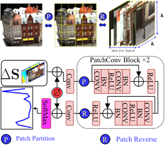
For simplicity, we transform the sampling problem into a probability distribution problem. We purpose a SampleNet $\mathcal{F}$ to predict the non-uniform sampling distribution with learning:

where $\mathbf{I}_{1}$ is the reference view, $\mathbf{\hat{L}}_{k-1}$ is the depth map of previous stage. We define the Sample Cost $\Delta\mathbf{S}_{k-1}$ to quantify the quality of sampling at the previous stage and constrain the distribution of sampling at the next stage, which is calculated from the normalized standard deviation:

When the standard deviation $\sqrt{(\mathbf{L}_{k-1}-\mathbf{\hat{L}}_{k-1})^{2}\cdot\mathbf{P}_{k-1}}$ limit to 0, it means that all planes are distributed around the depth maps $\mathbf{\hat{L}}_{k-1}$. The depth map $\mathbf{L}_{k-1}$ and reference view $\mathbf{I}_{1}$ can also regularize the sampling distribution. In our experiments, SampleNet can well couple the relationship between them. There is difference in the contribution to the accuracy, $\Delta\mathbf{S}_{k-1}$ and $\mathbf{L}_{k-1}$ contributes the most. It will be discussed in Sec. 3.4.

From the sampling distribution $P_{k}$, we have all the interval between the plane $\Delta d_{k}$:

and the sampling depth of $j$-th plane $\mathbf{L}_{k,j}$ based on the previous estimate is:

Specially, $-\frac{\sum^{D_{k}/2-1}_{j=0}\Delta d_{k,j}+\sum^{D_{k}/2}_{j=0}\Delta d_{k,j}}{2}$ makes the previous depth in the center of all planes which is important for coarse-to-fine at next stage and training.

The 3D CNN is U-Net with the 3D convolution, but the skip connections are added. In the encoder, we downsample the input resolution form $H\times W$ to $\frac{H}{8}\times\frac{W}{8}$ and the decoder back to the input resolution by upsampling. The output layers, followed by SoftMax, output the depth probability $\mathbf{P}_{k,j}$.

We use the 3D CNN to regularize the 3D cost volume $\Delta\mathbf{C}_{k,j}$ to get the depth probability $\mathbf{P}_{k,j}$. The depth map $\hat{L}_{k}$ of $k$-th stage is:

For supervised learning our SuperMVS, we use four smooth L1 losses girshick2015 to build the loss function:

where $\lambda_{1}=0.25,\lambda_{2}=0.5,\lambda_{3}=1,\lambda_{4}=2$ and the $L^{gt}_{k}$ is the ground truth of $k$-th stage.

The DTU dataset journals/ijcv/AanaesJVTD16 is a large-scale indoor MVS dataset with 124 different scenes. It includes images with different views and lighting, camera parameters and depth maps. It also provides the 3D point cloud data for all scenes. We use it to train, test and validation the model. The dataset split is the same as that in other methods defined at JiGZLF17. The Tanks & Temples dataset journals/tog/KnapitschPZK17 consists of realistic indoor and outdoor scenes. It divided intermediate and advanced datasets. In our work, we train the SuperMVS on DTU training set, then test it on the DTU evaluation set and the intermediate set of Tanks & Temples dataset.

We set the images resolution to $[H=512,~W=640]$ and the number of input images to $N=5$. The number of hypothesis plane is $D_{1}=48$, $D_{2}=16$, $D_{3}=8$ and $D_{4}=8$. The scale of hypothesis range is $R_{2}=0.38$, $R_{3}=0.16$ and $R_{4}=0.04$. All stages use our non-uniform sampling method to build the cost volume, except for the first stage use the uniform sampling at $\Delta\mathbf{R}$ for initialize the depth. We implement our model with Pytorch paszke2019pytorch and train it on $2\times$ Nvidia RTX 3090 GPUs with batch size of 4 per GPU. We employ the Adam kingma2014adam optimizer with an initial learning rate $0.0016$ to train for $26$ epoch, where the learning rate shcedule is divided by $2$ every two epochs starting from $10^{th}$ epoch.

We compare our results with other state-of-the-art of learning-based methods as the baseline in Table.1. It is worth noting that most of them use the uniform sampling method in the table. Our method outperforms other algorithms on completeness and overall. We also list the number of planes set by different algorithms when the cost volume resolution is $\frac{H}{4}\times\frac{W}{4}\times planes$. We can see that the number of planes directly affects the accuracy, memory and runtime based on the uniform sampling method. Our model reduces computation and achieves competitive performance by using the least number of planes 16. Compared with R-MVSNet conf/cvpr/0008LLSFQ19, large number of planes 512 leads to longer runtime 3.72s, our method reduces by 3.50s. Compared with UCS-Net conf/cvpr/ChengXZLLRS20, the number of planes 64 needs 6.9GB more memory, our method reduces the memory by 1.5GB. Our method also achieves significant improvement in overall, comparing to CasMVSNet conf/cvpr/GuFZDTT20 and UCS-Net, improving up 0.030mm and 0.019mm, respectively. In Fig.4, we compare the qualitative of point cloud with R-MVSNet, CasMVSNet and UCS-Net. Our method has less noise and higher completeness.

References

- (1) Henrik Aanæs, Rasmus Ramsbøl Jensen, George Vogiatzis, Engin Tola, and Anders Bjorholm Dahl. Large-scale data for multiple-view stereopsis. Int. J. Comput. Vis., 120(2):153–168, 2016.
- (2) Abien Fred Agarap. Deep learning using rectified linear units (relu), 2018. cite arxiv:1803.08375Comment: 7 pages, 11 figures, 9 tables.
- (3) Neill D. F. Campbell, George Vogiatzis, Carlos Hernández, and Roberto Cipolla. Using multiple hypotheses to improve depth-maps for multi-view stereo. In David A. Forsyth, Philip H. S. Torr, and Andrew Zisserman, editors, ECCV (1), volume 5302 of Lecture Notes in Computer Science, pages 766–779. Springer, 2008.
- (4) Rui Chen, Songfang Han, Jing Xu, and Hao Su. Point-based multi-view stereo network. In ICCV, pages 1538–1547. IEEE, 2019.
- (5) Shuo Cheng, Zexiang Xu, Shilin Zhu, Zhuwen Li, Li Erran Li, Ravi Ramamoorthi, and Hao Su. Deep stereo using adaptive thin volume representation with uncertainty awareness. In CVPR, pages 2521–2531. IEEE, 2020.
- (6) Yasutaka Furukawa and Jean Ponce. Accurate, dense, and robust multiview stereopsis. IEEE Trans. Pattern Anal. Mach. Intell., 32(8):1362–1376, 2010.
- (7) Silvano Galliani, Katrin Lasinger, and Konrad Schindler. Massively parallel multiview stereopsis by surface normal diffusion. In ICCV, pages 873–881. IEEE Computer Society, 2015.
- (8) Ross Girshick. Fast r-cnn, 2015. cite arxiv:1504.08083Comment: To appear in ICCV 2015.
- (9) Xiaodong Gu, Zhiwen Fan, Siyu Zhu, Zuozhuo Dai, Feitong Tan, and Ping Tan. Cascade cost volume for high-resolution multi-view stereo and stereo matching. In CVPR, pages 2492–2501. IEEE, 2020.
- (10) Kaiming He, Xiangyu Zhang, Shaoqing Ren, and Jian Sun. Deep residual learning for image recognition, 2015. cite arxiv:1512.03385Comment: Tech report.
- (11) Sergey Ioffe and Christian Szegedy. Batch normalization: Accelerating deep network training by reducing internal covariate shift. arXiv preprint arxiv:1502.03167, 2015.
- (12) Mengqi Ji, Juergen Gall, Haitian Zheng, Yebin Liu, and Lu Fang. Surfacenet: An end-to-end 3d neural network for multiview stereopsis. In ICCV, pages 2326–2334. IEEE Computer Society, 2017.
- (13) Diederik P Kingma and Jimmy Ba. Adam: A method for stochastic optimization. arXiv preprint arXiv:1412.6980, 2014.
- (14) Arno Knapitsch, Jaesik Park, Qian-Yi Zhou, and Vladlen Koltun. Tanks and temples: benchmarking large-scale scene reconstruction. ACM Trans. Graph., 36(4):78:1–78:13, 2017.
- (15) Ze Liu, Yutong Lin, Yue Cao, Han Hu, Yixuan Wei, Zheng Zhang, Stephen Lin, and Baining Guo. Swin transformer: Hierarchical vision transformer using shifted windows, 2021. cite arxiv:2103.14030Comment: The first 4 authors contribute equally.
- (16) Adam Paszke, Sam Gross, Francisco Massa, Adam Lerer, James Bradbury, Gregory Chanan, Trevor Killeen, Zeming Lin, Natalia Gimelshein, Luca Antiga, Alban Desmaison, Andreas Köpf, Edward Yang, Zach DeVito, Martin Raison, Alykhan Tejani, Sasank Chilamkurthy, Benoit Steiner, Lu Fang, Junjie Bai, and Soumith Chintala. Pytorch: An imperative style, high-performance deep learning library, 2019. cite arxiv:1912.01703Comment: 12 pages, 3 figures, NeurIPS 2019.
- (17) Olaf Ronneberger, Philipp Fischer, and Thomas Brox. U-net: Convolutional networks for biomedical image segmentation, 2015. cite arxiv:1505.04597Comment: conditionally accepted at MICCAI 2015.
- (18) Johannes L. Schönberger and Jan-Michael Frahm. Structure-from-motion revisited. In CVPR, pages 4104–4113. IEEE Computer Society, 2016.
- (19) Johannes L. Schönberger, Enliang Zheng, Jan-Michael Frahm, and Marc Pollefeys. Pixelwise view selection for unstructured multi-view stereo. In Bastian Leibe, Jiri Matas, Nicu Sebe, and Max Welling, editors, ECCV (3), volume 9907 of Lecture Notes in Computer Science, pages 501–518. Springer, 2016.
- (20) Engin Tola, Christoph Strecha, and Pascal Fua. Efficient large-scale multi-view stereo for ultra high-resolution image sets. Mach. Vis. Appl., 23(5):903–920, 2012.
- (21) Fangjinhua Wang, Silvano Galliani, Christoph Vogel, Pablo Speciale, and Marc Pollefeys. Patchmatchnet: Learned multi-view patchmatch stereo, 2021.
- (22) Jiayu Yang, Wei Mao, Jose M. Alvarez, and Miaomiao Liu. Cost volume pyramid based depth inference for multi-view stereo. In CVPR, pages 4876–4885. IEEE, 2020.
- (23) Yao Yao, Zixin Luo, Shiwei Li, Tian Fang, and Long Quan. Mvsnet: Depth inference for unstructured multi-view stereo. In Vittorio Ferrari, Martial Hebert, Cristian Sminchisescu, and Yair Weiss, editors, ECCV (8), volume 11212 of Lecture Notes in Computer Science, pages 785–801. Springer, 2018.
- (24) Yao Yao, Zixin Luo, Shiwei Li, Tianwei Shen, Tian Fang, and Long Quan. Recurrent mvsnet for high-resolution multi-view stereo depth inference. In CVPR, pages 5525–5534. Computer Vision Foundation / IEEE, 2019.
- (25) Zehao Yu and Shenghua Gao. Fast-mvsnet: Sparse-to-dense multi-view stereo with learned propagation and gauss-newton refinement. In CVPR, pages 1946–1955. IEEE, 2020.