Budget-Constrained Reinforcement of Ranked Objects

Ranking systems, and in particular their capability for manipulation, have been extensively studied Cheng and Friedman 2005, Altman and Tennenholtz 2006, Altman and Tennenholtz 2007, Altman and Tennenholtz 2010. Getting optimal influence for a given budget, or vice versa, was considered by Feldman et al. 2007 and Alon et al. 2012, and in bidding for advertising, by Wu et al. 2018. Manipulating elections is a closely-related subject, e.g. Conitzer et al. 2007.

Our original motivation was to investigate competitive reinforcement games, in which two principals have separate budgets to support a set of ranked entries. What is sought are reinforcement strategies in equilibrium. Stated thus, the problem is related to Colonel Blotto games, due to Borel 1953, in which two colonels partition their men into detachments, assigned to a set of contested hills, each won by the colonel who assigned more men to that hill. An even better fit are General Lotto games Hart 2008, where after the partition by each side into detachments, one detachment is chosen at random from each army, and the bigger one wins.

A solution of such a problem, with asymmetric budgets, is given in Sahuguet and Persico 2006, where it is framed as an allocation problem in competitive campaign spending. Hart 2008 represents the partition of resources as a probability distribution, demonstrating that this reduces the problem to a game between probability distributions.

While studying this background, we realized that the non-competitive reinforcement problem is far from trivial; it is more elementary and of more practical value than the competitive one, and to the best of our knowledge it has not been addressed in the literature.

The rest of this paper is organized as follows. Section 2 describes the reinforcement problem. Section 3 details our method and algorithms and provides a numerical example. In Section 4 we characterize the optimal solution of the problem, and prove the correctness of the algorithms given. In Section 5 we offer concluding remarks.

The method is based on the following idea. The optimal solution is to implement all possible reinforcements where the complement’s average density between initial and final score exceeds a threshold, called $\alpha$ in the algorithms. Plotted on the complement’s c.d.f., this means all reinforcements are made across chords steeper than $\alpha$. In practice, we select scores for which the complement’s p.d.f. is $\alpha$, calling them target scores, and each is the endpoint of a segment of scores whose chord’s gradient to the target score is at least $\alpha$. All supported entries (in $\mathcal{A}$) whose score falls in any such segment is reinforced to meet the corresponding segment end/target score.

All this is implemented by the Basic Algorithm (Algorithm 1 below) for a given parameter $\alpha$. The algorithm has no control over the budget it uses, which is a function $\BDG_{\alpha}$ of its parameter. However, as will be proved later (Proposition 3), this budget is non-increasing in $\alpha$.

Harnessing this monotonicity, the Iterative Algorithm (Algorithm 2 below), iteratively applies Algorithm 1 in a binary search to find an $\alpha$ parameter for which $\BDG_{\alpha}$ most closely approaches the given budget without exceeding it. Based on this, it constructs the sought-after optimal solution.

The algorithm is equally applicable to exact (list of values) and statistical (analytical formula) representations of the complement. For the latter, implementing the algorithm may need unspecified analytical or numerical steps (e.g., finding solutions of $f_{\bm{c}}(x)=\alpha$).

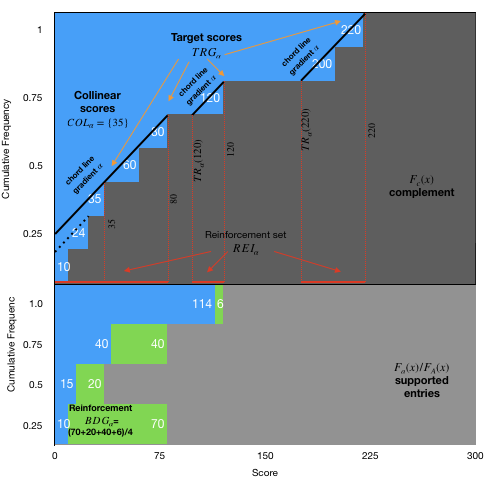
Consider the set of entries detailed in Table 1. There are $12$ entries, ranked by score (1st column), $4$ of which are supported, and $8$ in the complement. The c.d.f.’s of the supported and complement entries are shown in the 2nd and 3rd columns, respectively. See in Figure 2 a plot of the two c.d.f.’s. As the distributions are discrete, the c.d.f.’s are step functions. The top part of Figure 2 plots the complement’s c.d.f., in dark grey. The bottom part plots the supported entries’ c.d.f. in grey and green. The $x$-axis (scores) is common to both c.d.f.’s.

The figure shows the optimal reinforcement when the total budget $|\mathcal{A}|p_{A}$ equals $181$.

We draw parallel chord lines, whose common gradient is a given $\alpha$, from the top of each step in the complement’s c.d.f.. Each chord line extends to the left, up to where it intersects with the c.d.f. plot, or until it intersects with the $y$-axis, whichever comes first. The score ($x$ value) of this intersection is called the trace of the chord line. E.g., the vertical dotted red line labeled $\TR_{\alpha}(220)$ in the figure is the trace of complement score $220$.

The set of scores that lie between complement scores and their traces is called the reinforcement set. It is marked in Figure 2 in three red segments on the $x$-axis. Note that only three complement scores contribute to the reinforcement set: $80,120$ and $220$. The chord line of complement score $24$ (marked by a dotted black line), for example, does not contribute to the reinforcement set, because it is wholly contained in the contribution of complement score $80$. The same is true for the rest of the chord lines (not shown).

The 3 complement scores who do contribute to the reinforcement set are the target scores. Every supported score who is reinforced by the method, is reinforced to one of the target scores, and specifically to the next-higher target score.

The supported scores that are reinforced are those whose score is in the reinforcement set. Moving our attention in Figure 2 to the bottom plot, we see that all $4$ supported entries are in the reinforcement set, a coincidence. The green plot shows the reinforcement, with the number near the green/grey boundary showing the reinforcement for each supported entry. The total reinforcement, i.e., budget, is $70+65+40+6=181$, as required. Note that the budget is proportional to the green area.

However, if we are given a target budget, we have no direct method of determining which chord line gradient $\alpha$ results in such a budget. We have to search for it, and we do so using binary search, as described in the Iterative Algorithm.

A complicating, but unavoidable factor is the possibility of collinearity, where a score lies exactly on another score’s chord line (for some gradient $\alpha$). In Figure 3 we see a picture that is almost identical to that of Figure 2, except that the gradient $\alpha$ is steeper just enough to make score $80$’s chord line meet the complement’s c.d.f. at the top of the step for score $35$, with the result that the chord lines for complement scores $80$ and $35$ are collinear.

As in Figure 2, all scores from $0$ to $80$ are in the reinforcement set. Supported scores $10,15$ and $40$ should therefore be reinforced to the next-higher target score. But for the scores below $35$ ($10$ and $15$), which is the next-higher target score, $35$ or $80$? The answer given by our analysis is: either. In Figure 3 score $10$ is reinforced to $80$ and score $15$ is reinforced to $35$, for a total budget of $136$. An equally optimal solution with the same budget is to promote score $10$ to $35$ and score $15$ to $80$. Since these two scores can be reinforced to either $35$ or $80$, this collinear gradient $\alpha$ is responsible for the optimal solution for budgets anywhere from $25+20+40+6=91$ to $70+65+40+6=181$. Given a budget of, e.g., $150$, our optimal solution would be as in Figure 3, leaving $150-136=14$ unused.

The reader will notice that the upper bound of this range is $181$, which is the same as the Figure 2 budget. This is because the gradient $\alpha$ of Figure 2 can be perturbed without change: So long as the chord lines do not touch a new score, the solution, and so the budget is unchanged.

If $\bm{c}$ has no atom at $x$, then for $\epsilon>0$, $\lim_{\epsilon\to 0}C_{x}^{x+\epsilon}$ and $\lim_{\epsilon\to 0}C_{x}^{x-\epsilon}$ both exist, and are called, respectively, the left and right density of $\bm{c}$ at $x$. If $\bm{c}$’s c.d.f. is differentiable at $x$, they are equal.

The basic algorithm is detailed in Algorithm 1. Following are notes referred to in the algorithm.

1. 1.

   The parameter $\alpha$, in the context of p.d.f. $f_{\bm{c}}$, signifies a threshold density, while in the context of c.d.f. $F_{\bm{c}}$, signifies a gradient, i.e., the slope of a segment connecting two points on the c.d.f., or, equivalently, the average density between their scores/$x$-values.

2. 2.

   In the exact problem, $\BDG_{\alpha}$ is a step function of $\alpha$, due to Note 6. $\NEXT_{\alpha}$ is the next-lower gradient $\alpha$ at which $\BDG_{\alpha}$ changes. This is the gradient where the chord lines of the target scores, sweeping clockwise (lower $\alpha$) would meet a new entry (supported or complement) score. In Figures 2 and 3, this is the slope from target score $80$ to $120$, i.e., $\NEXT_{\alpha}=C_{80}^{120}$. The chord is marked in Figure 2 by a dotted green line. When no such entry exists, we set $\NEXT_{\alpha}=0$.

   In the statistical problem $\NEXT_{\alpha}=0$ indicates that the entire complement c.d.f. is in the reinforcement set. This can be true only if $\bm{c}$ has bounded support.

   In both versions of the problem, $\NEXT_{\alpha}=0$ indicates that the current $\alpha$ uses the maximum possible budget: All supported entries outrank all complement entries.

3. 3.

   The scores in $\CTR_{\alpha}$ are characterized by the fact that the chord line of gradient $\alpha$ at $x$ is entirely on or above the complement’s c.d.f. for a neighborhood surrounding both sides of $x$ (see Figure 2).

   $\CTR_{\alpha}$ includes

   • •

     All solutions $x$ of $f_{\bm{c}}(x)=\alpha$ where the density declines right of $x$. Equivalently, where the complement’s c.d.f. tangent at $x$ is $\alpha$ and the c.d.f. is concave at $x$.

   • •

     All scores $x$ where $\bm{c}$ has an atom.

   • •

     Scores $x$ where $f_{\bm{c}}(x)$ has a non-atom discontinuity, with the left-density $\geq\alpha$ and the right-density $\leq\alpha$.

   The set of candidate target scores is finite, except when the complement distribution is uniform with density $\alpha$ in all or part of its support. In this exception, the $\alpha$-segments are all empty, so $\TRG_{\alpha}$ is always finite.

   For the exact problem, the complement’s c.d.f. is a step function, and the density is $0$ except at the steps. By the above definition, $\CTR_{\alpha}$ is the set of scores of all steps $x$, and furthermore, this set does not depend on $\alpha$ (but the set $\TRG_{\alpha}\subseteq\CTR_{\alpha}$ of target scores will, in general, depend on $\alpha$).

4. 4.

   Since all chord lines have the same slope $\alpha$, they do not intersect. Therefore, every pair of $\alpha$-segments are either disjoint or one is wholly contained in the other. Since $\TRG_{\alpha}$ includes only candidate target scores whose $\alpha$-segments are mutually disjoint, we can skip candidate target scores that are larger than the last target score’s trace ($\LTR$), since their $\alpha$-segment must be wholly contained in the last $\alpha$-segment.

5. 5.

   For a collinear target score $z$, which is a trace of another target score $x$, the chords at $x$ and $z$ are necessarily collinear, and the endpoint of $z$’s $\alpha$-segment is the starting point of $x$’s $\alpha$-segment.

   This is illustrated in Figure 3, where gradient $\alpha$ is such that the chord lines of scores $35$ and $80$ are collinear.

   On the other hand, in Figures 2 and 3, no supported scores coincide with a chord line trace, so they have no collinear source scores.

   The presence of collinear scores, and certainly many of them, for any given value of $\alpha$, is exceptional. It requires the coincidence of, for example, a score in $\supp(\bm{a})$ coinciding with a trace of an atom in $\bm{c}$, or of chord gradients between two $\bm{c}$ atoms being equal to $\alpha$. There is a finite number of values of $\alpha$ with any collinear scores.

6. 6.

   The total budget used by Algorithm 1 is ³³ 3 Here and later $\HIGH(x)$ is shorthand for $\HIGH_{\REI_{\alpha}}(x)$. See Definition 4.

   	$\displaystyle\BDG_{\alpha}$	$\displaystyle:=\int_{x\in\REI_{\alpha}\setminus\COL_{\alpha}}[\HIGH(x)-x]f_{\bm{a}}(x)dx$
   		$\displaystyle=\frac{1}{|\mathcal{A}|}\sum_{z\in\mathcal{A}\land r_{z}\in\REI_{\alpha}\setminus\COL_{\alpha}}[\HIGH(r_{z})-r_{z}]$

7. 7.

   The resulting $\alpha$-reinforcement set contains all reinforced scores and is

   $$\REI_{\alpha}:=\bigcup_{x\in\CTR_{\alpha}}[\TR_{\alpha}(x),x)=\bigcup_{x\in\TRG_{\alpha}}[\TR_{\alpha}(x),x)$$

The Iterative Algorithm, detailed in Algorithm 2, applies the Basic Algorithm repeatedly using binary search to find the optimal solution for budget $p_{A}$, relying on the role played by the collinear scores, and on the monotonicity of $\BDG_{\alpha}$, properties that are stated and proved in Section 4 below. The reader is referred to Section 4.2 as to the method used by the algorithm and its justification.

In this section, we demonstrate the correctness of the algorithms given in Section 3.

The following proposition shows that there is a dichotomy between two types of chords from a target score: All chords to the left (lower score) are steeper than all chords to the right, as well as to scores supported in $\bm{A}$. When $F_{\bm{c}}$ is differentiable at the target score, the dichotomy’s boundary is the tangent slope at the target score.

However, since a score may belong to both types, i.e., be both left of a target score, and belong to $\supp(\bm{A})$, we immediately conclude from Proposition 2:

We can now characterize the optimal solution.

Given a threshold density $\alpha$, Theorem 4.1 almost completely characterizes $\bm{A}$ after an optimal reinforcement: It shows that entries in $\mathcal{A}$ whose score falls in one of the $\alpha$-segments of a target score are reinforced to meet a target score in that segment. The only open question it leaves is whether that target score is the segment’s high endpoint, or some other score that is on the chord line (this question, when relevant, is resolved by Algorithm 2).

This proves the correctness of Algorithm 1.

The Iterative Algorithm applies the Basic Algorithm repeatedly using numeric methods (binary search) to find the optimal (or $\epsilon$-optimal, for the statistical version) solution for budget $p_{A}$, relying on the role played by the collinear scores, as described in Theorem 4.1, and on the monotonicity of $\BDG_{\alpha}$ and of $\REI_{\alpha}$, stated in the following proposition.

The monotonicity of $\BDG_{\alpha}$ allows an $\epsilon$-optimal $\alpha$ to be found by binary search. Moreover, for the exact problem, the optimal solution can be found: $\BDG_{\alpha}$ is a non-increasing step function of $\alpha$, and the Basic Algorithm calculates the lower end of the step whose budget is $\BDG_{\alpha}$, $\NEXT_{\alpha}$. Whenever binary search halves the search interval, and the middle $\alpha$ needs a budget which is still short of the target $p_{A}$, $\NEXT_{\alpha}$, rather than the middle $\alpha$ becomes the lower end of the search interval. In combination with the binary search, this guarantees that the search will find the gradient $\alpha$ for the required budget $p_{A}$.

Theorem 4.1 allows for optimal solutions that are not constructed by the Basic Algorithm, where scores are reinforced to scores on the chord line that are not nearest. The solution remains optimal (though not for the same budget) if any entry that was reinforced to (or was originally at) a collinear score ($\in\COL_{\alpha}$) is promoted to the next-higher target score.

Furthermore, if gradient $\alpha$ is slightly decreased to $\alpha-\epsilon$, for sufficiently small $\epsilon>0$, the collinear scores disappear, and all entries that were reinforced by Algorithm 1 to a collinear score $y$ are now reinforced to the next target score that is not in $\in\COL_{\alpha}$. Mark it $\HIGHER(y)$. E.g., in Figure 3, scores $35$ and $80$ are collinear, so $\HIGHER(x)=80$, for every score in $[\TR_{\alpha}(80),80)$. We have a discontinuity in $\BDG_{\alpha}$ of size

It follows that for all budgets between $\BDG_{\alpha}$ and $\lim_{\epsilon\to 0}\BDG_{\alpha-\epsilon}$, the optimal solution has threshold density $\alpha$. This solution is implemented by first finding the basic solution with Algorithm 1, and then “promoting” entries on collinear scores to a higher target score as much as the budget allows.

Since we seek an integral target distribution, in which an integral number of entries are reinforced, and the promotion interval, i.e., the distance between target scores, is fixed, the problem amounts to finding an integral number for each of several given intervals. This adds, as closely as possible, to the budget $p_{A}$, without exceeding it. This is essentially a bounded knapsack problem, which, as is well-known, is NP-complete in $|\COL_{\alpha}|$, and pseudo-polynomial in $p_{A}$.

These considerations are handled by steps 8 to 10 of Algorithm 2, according to the number of collinear scores $|\COL_{\alpha}|$ at the end of the binary search. If there are none, there is nothing to do, and the step 7 result is the solution. When $|\COL_{\alpha}|=1$, the knapsack problem is trivial, with only one kind of object. We find the number of entries to promote by dividing the knapsack size (i.e., the residual budget $p_{A}-\BDG_{\alpha}$) by the size of the object (the distance $\HIGHER(y)-y$, where $y$ is the sole collinear score), as done in Algorithm 2, step 9.

When $|\COL_{\alpha}|>1$, one may use any textbook solution of the bounded knapsack problem, e.g. Martello 1990. While this problem is NP-complete in the number of collinear scores (but pseudo-polynomial in the residual budget), it is safe to assume that $|\COL_{\alpha}|$ is bounded: Indeed as noted in Note 5, there is only a finite number of values of $\alpha$, a real variable, for which there are any collinear scores, so $|\COL_{\alpha}|\leq 1$ almost surely.

In the exact problem, the algorithm’s running time depends on the total number of entries ranked $n:=|\mathcal{W}|=|\mathcal{A}|+|\mathcal{C}|$, and on the range and resolution of the entries $\mathcal{W}$.

The running time of the Basic Algorithm is linear, i.e., $O(n)$ (assuming the ranking system already ranks them by score, otherwise the running time, including sort, is $O(n\log n)$). This is clear from the fact that the number of candidate target scores $|\CTR_{\alpha}|$ is at most $|\mathcal{C}|<n$, and for each, at most two chord gradients from it are computed (as starting point and as ending point). The number of operations performed on each entry in $\mathcal{A}$ is at most one, if it is reinforced.

The Basic Algorithm is executed several times in the Iterative Algorithm, so to find the total running time, we need to cap the number of iterations. The Iterative Algorithm starts with $\overline{\alpha}$ and $\underline{\alpha}$ whose traces are in the range of scores $\RANGE(\mathcal{W})$, defined in (7). Using binary search, this range is cut in half every iteration, and ultimately it may need to be small enough to contain a single score, i.e., it should be smaller than the resolution of scores $\RES(\mathcal{W})$, defined in (8). The number of iterations required is $O\Big(\log\frac{\RANGE(\mathcal{W})}{\RES(\mathcal{W})}\Big)$, and the total running time (for bounded $|\COL_{\alpha}|$) is

When $\bm{c}$ has a piecewise-differentiable and unimodal probability density, this leads to an easy solution: For every threshold $\alpha$ there is exactly one candidate target score, and no collinear target scores. There is at most one collinear source score, the trace of the only target score.

By unimodal, we mean a p.d.f. that has a single maximum at $M\geq 0$, and is strictly increasing for $x<M$ and decreasing for $x>M$, strictly so when the density is non-zero.

Most commonly-used continuous distributions of a positive random value are unimodal: Exponential, log-normal, Gamma and power law distributions. A notable exception is the uniform distribution.

References

- (1)
- Alon et al. (2012) Noga Alon, Iftah Gamzu, and Moshe Tennenholtz. 2012. Optimizing budget allocation among channels and influencers. In Proceedings of the 21st international conference on World Wide Web. ACM, 381–388.
- Altman and Tennenholtz (2006) Alon Altman and Moshe Tennenholtz. 2006. Quantifying incentive compatibility of ranking systems. In PROCEEDINGS OF THE NATIONAL CONFERENCE ON ARTIFICIAL INTELLIGENCE, Vol. 21. Menlo Park, CA; Cambridge, MA; London; AAAI Press; MIT Press; 1999, 586.
- Altman and Tennenholtz (2007) Alon Altman and Moshe Tennenholtz. 2007. Incentive compatible ranking systems. In Proceedings of the 6th international joint conference on Autonomous agents and multiagent systems. ACM, 84.
- Altman and Tennenholtz (2010) Alon Altman and Moshe Tennenholtz. 2010. An axiomatic approach to personalized ranking systems. Journal of the ACM (JACM) 57, 4 (2010), 26.
- Borel (1953) Emile Borel. 1953. The theory of play and integral equations with skew symmetric kernels. Econometrica: journal of the Econometric Society (1953), 97–100.
- Cheng and Friedman (2005) Alice Cheng and Eric Friedman. 2005. Sybilproof reputation mechanisms. In Proceedings of the 2005 ACM SIGCOMM workshop on Economics of peer-to-peer systems. ACM, 128–132.
- Conitzer et al. (2007) Vincent Conitzer, Tuomas Sandholm, and Jérôme Lang. 2007. When are elections with few candidates hard to manipulate? Journal of the ACM (JACM) 54, 3 (2007), 14.
- Feldman et al. (2007) Jon Feldman, Shan Muthukrishnan, Martin Pal, and Cliff Stein. 2007. Budget optimization in search-based advertising auctions. In Proceedings of the 8th ACM conference on Electronic commerce. ACM, 40–49.
- Hart (2008) Sergiu Hart. 2008. Discrete Colonel Blotto and general lotto games. International Journal of Game Theory 36, 3-4 (2008), 441–460.
- Martello (1990) Silvano Martello. 1990. Knapsack problems: algorithms and computer implementations. Wiley-Interscience series in discrete mathematics and optimiza tion (1990).
- Sahuguet and Persico (2006) Nicolas Sahuguet and Nicola Persico. 2006. Campaign spending regulation in a model of redistributive politics. Economic Theory 28, 1 (2006), 95–124.
- Wu et al. (2018) Di Wu, Xiujun Chen, Xun Yang, Hao Wang, Qing Tan, Xiaoxun Zhang, Jian Xu, and Kun Gai. 2018. Budget constrained bidding by model-free reinforcement learning in display advertising. In Proceedings of the 27th ACM International Conference on Information and Knowledge Management. ACM, 1443–1451.