Group pattern detection of longitudinal data using functional statistics

Functional Data Setting Let $\Omega$ be a population space of statistical units ($\omega\in\Omega$) and $s_{n}=\{\omega_{1},\omega_{2},\dots,\omega_{n}\}$ be a random sample of size $n$ drawn from $\Omega$. Let $\mathbf{Y}$ be a $L_{2}$-continuous multivariate stochastic process defined on $\Omega$ associating to a set of $D$ curves, $D\geq 2$, where each curve in one dimension defined on a given finite interval $\mathcal{T}=[0,T],0<T<\infty$, i.e., $\mathbf{Y}(\omega)=[\mathbf{y}_{\omega,1}(t),\dots,\mathbf{y}_{\omega,D}(t)]^{T}$ (denoted as $\mathbf{Y}=(\mathbf{y}_{1},\dots,\mathbf{y}_{D})^{T}$ for simplicity), $t\in\mathcal{T}$, such that

The observations of $\mathbf{Y}$ on the sample $s_{n}$ are called multivariate functional data, providing independent realizations as samples $\{\mathbf{Y}(\omega_{1}),\dots,\mathbf{Y}(\omega_{n})\}$ with multivariate curves jacques2012clustering. The mean functions of $\mathbf{y}_{d}$ and $\mathbf{Y}$ are

The covariance operator of $\mathbf{Y}$ is then defined as an integral operator $\mathcal{C}$ with kernel

where $\otimes$ is the tensor product on $\mathbb{R}^{D}$. Thus, $\mathbf{C}(t,s)$ is a $D\times D$ matrix with elements

Functional Principal Component Analysis (FPCA) Under the hypothesis of $L_{2}$-continuity, $\mathcal{C}$ is an Hilbert-Schmidt operator, i.e., it is compact and self-adjoint. Meanwhile, the spectral analysis of $C$ provides a countable set of positive eigenvalues $\{\eta_{j,j\geq 1}\}$ associated to an orthonormal basis of multivariate eigen-functions $\{\mathbf{f}_{j,j\geq 1}\}$, $\mathbf{f}_{j}=[\mathbf{f}_{j,1},\dots,\mathbf{f}_{j,D}]^{T}$, such that

with $\eta_{1}\geq\eta_{2}\geq\dots$ and $\langle\mathbf{f}_{i},\mathbf{f}_{j}\rangle_{\{L_{2}([0,T])\}^{D}}=\delta_{i,j}$ with $\delta_{i,j}=1$ if $i=j$, otherwise $\delta_{i,j}=0$ berrendero2011principal. Assume that the principal components $\eta_{j}$ of $\mathbf{Y}$ are zero-mean random variables, as the projections of $\mathbf{Y}$ on the $j$th eigenfunction of $\mathbf{C}$:

which means $\mathbf{Y}(t)$ varies around the mean function with random amplitude variations in the directions of $\{\mathbf{f}_{j}\}_{j\geq 1}$. Therefore, following Karhunen-Loeve expansion, it holds that

are the best approximations of this form under the mean square criterion.

Functional Registration In practice, it is essential to align observed functions into a common registered internal timeline to isolate the phase variability of the functions, but keeping, at the same time, the amplitude-phase unchanged to maintain the information under interests. The phase variation is normally represented by a random change of time scale, which is mostly a non-linear transformation. We use the warping functions $T_{i}:[0,T]\rightarrow[0,T],i=1,\dots,n$, assuming that they are increasing functions independent of amplitude variation. They map unregistered chronological time $t_{i}^{*}$ to registered internal time $t$ so that $T_{i}^{-1}(t_{i}^{*})=t$, with $E[T_{i}(t)]=t$. The observed time-warped curves, represented through a Karhunen-Loeve expansion based on a functional basis $\mathbf{f}_{j,d}$, are

The literature is rich of proper methods to do this, and a more in-depth review would be beyond the scope of this report. Briefly speaking, we followed the principal components based registration method wrobel2019register with a generative process, by alternating the process between using the generalized FPCA to calculate template functions and estimating smooth time warping functions that map observed curves to templates ¹¹ 1 Codes are available in the R package ”registr” wrobel2018register.

Approximation into finite basis of functions Often in practice, data are observed at discrete time points and with some noise. In order to get the functional feature of data, researchers normally use some smoothing and interpolation methods to rebuild the consecutive function from the discrete data, while assuming that the latent function belongs to a finite dimensional functional space spanned by some functional basis. In this way, functional data objects are constructed from time series data by specifying a set of basis functions and a set of coefficients defining a linear combination of these basis functions. For non-periodic time series, B-spline basis functions which contain polynomial segments jointed end-to-end at argument values are frequently considered, benefiting the most from fast computational ability and great flexibility ramsay1997functional.

Let $y_{g,d,k}(t)$ denote the evolution of one specific variate $d\in\{1,\dots,D\}$ in sample $k\in\{1,\dots,K\}$ for one group $g\in\{0,\dots,G\}$. We can assume that

where $\mu_{d,0}(t)$ is the grand mean function independent from groups. The term $\alpha_{d,g}(t)$ is the additional effect function of group $g$ on the considered variate $d$, while $\epsilon_{g,d,k}(t)$ represents the unexplained zero-mean variation, specific of the $k$-th sample within group $g$. In order to identify the parameter functions uniquely, we require the constraint $\sum\limits_{g=0}^{G}\alpha_{d,g}(t)=0,\forall t.$

By grouping the samples from the same group, we can define a $(GK+1)\times(G+1)$ design matrix $\mathbf{Z}_{d}$ for univariate model, with suitable 0 and 1 entries, as described in (ramsay1997functional, Section 9.2), and rewrite Equation (3) in matrix form

where

Here $\mathbf{\beta}_{d}$ is defined as the corresponding set of $G+1$ regression functions for mean and $G$ additional groups, and $\mathbf{\epsilon}_{d}$ is the matrix of noise with the same dimension of $\mathbf{y}_{d}$.

Following the notations above, we can write the multivariate matrix form for the multiple regression functions, as

where

Under the functional least squares fitting criterion on $R^{GDK\times T}$ space, we can estimate the parameters

where $\Theta(t)=(\theta_{1}(t),\dots,\theta_{q}(t),\dots,\theta_{Q}(t))^{T}$ denotes a linear combination of basis functions with $J_{\theta\theta}$ as the inner product of each pair of functional basis, and $\hat{\mathbf{B}}$ is the estimated coefficient matrix with

Here, $\mathbf{A}$ is the coefficient matrix of samples $\mathbf{Y}(t)$ with a fixed B-spline functional basis and more computation details in matrix format are shown in Appendix 3.1.

After establishing the model for functional evolution processes and estimating the additional parameter functions affected by group categories, next goal is to investigate whether and when group labels are significantly influencing the change of variables. ANOVA-related methods are suitable tools to determine the effects of independent categorical variables on continuous dependent variables, by comparing inter-group differences between centroids represented as the vectors of the mean values of the dependent variables. Moreover, in order to construct feasibly more general hypothesis tests for group means, contrasts, defined as a linear combination of regression coefficients where the values of the linear combination sum up to 0, are applied by specifying the values on different pairs of groups gradually.

For each subgroup of variable $d\in\{1,\dots,D\}$ and group $g\in\{0,\dots,G\}$, assume that the $k$-th sample curve in this subgroup $y_{d,g,k}(t)\sim\mathbb{N}(\mu_{d,g}(t),\sigma^{2}),k\in\{1,\dots,K\}$ with group mean $\mu_{d,g}(t)$ and constant variance $\sigma^{2}$, and therefore the subgroup sample mean $\overline{Y}_{d,g,\cdot}(t)=\frac{1}{K}\sum\limits_{k=1}^{K}y_{d,g,k}(t)\sim\mathbb{N}(\mu_{d,g}(t),\frac{\sigma^{2}}{K})$. Here denote $\mathbf{\mu}(t)$ as the sequence of subgroup means $\mu_{d,g}(t)$ for all $d\in\{1,\dots,D\}$ and $g\in\{0,\dots,G\}$. We construct one test for each pair of groups in comparison (one control group $g=0$ and another group under study $g=\tilde{g}$ for one variable $d$) and in $i$-th test ($i\in\{1,\dots,DG\}$) we design a vector $\mathbf{a}=[0,\dots,0,1,0,\dots,0,-1,0,\dots,0]$ in length $D(G+2)$ (same as the length of $\mathbf{\beta}(t)$ in last section) with the entries pointed to the pair of groups in comparison being 1 and -1 respectively, i.e., $a_{d(G+2)+2}=1$, $a_{d(G+2)+2+\tilde{g}}=-1$, and 0 in entries remained. We define the contrast in $i$-th test as $c=\mathbf{a}^{T}\mathbf{\mu}(t)=\alpha_{d,0}(t)-\alpha_{d,\tilde{g}}(t)=(\alpha_{d,0}(t)+\mu_{d,0})-(\alpha_{d,\tilde{g}}(t)+\mu_{d,0})$ for $DG$ different group comparisons, where the sum of weigths in $\mathbf{a}$ is zero, and then the difference of subgroup sample means $\overline{Y}_{d,0,\cdot}(t)-\overline{Y}_{d,\tilde{g},\cdot}(t)$ is an unbiased estimator of the contrast $c$. Following this setting, the null hypothesis at each time point $t$ for the control group and the group under study $\tilde{g}$ in variable $d$ is

and the related F statistics under null hypothesis is

where the sum of sample variances is $S_{p}^{2}=\frac{1}{N-DG}\sum\limits_{g=1}^{G}\sum\limits_{d=1}^{D}\sum\limits_{k=1}^{K}(y_{d,k,g}(t)-\overline{y}_{d,g,\cdot}(t))^{2}$ with sample size $N$. When assuming the functional data $y_{d,k,g}(t)$ as realizations of Gaussian processes, for any given $t\in\mathcal{T}$, $F_{d,\tilde{g}}(t)\sim F_{1,N-DG}$, where $F_{1,N-DG}$ denotes $F$-distribution with $1$ and $N-DG$ degrees of freedom.

The statistic $F_{d,\tilde{g}}(t)$ should be compared with a critical value of $F_{1,N-DG}$ for any predetermined significant level $\alpha$. The critical value of $F_{1,N-DG}(\alpha)$ represents the $\alpha$-fraction of rejection area, where $F_{1,N-DG}(\alpha)$ denotes the upper $100\alpha$ percentile of $F_{1,N-DG}$. We write the $1-\alpha$ quantile of the distribution of F statistic by $c_{1-\alpha}$, and given $c_{1-\alpha}$, we reject the null hypothesis when $F_{d,\tilde{g}}(t)>c_{1-\alpha}$, which indicates the dissimilarity of group means under comparison. First, we can test the statistic at all points of $\mathcal{T}$ using the same critical value from standard F-Distribution table with correlated degrees of freedom. Since complex assumptions and convoluted formula are not often satisfied in practice for most classic statistical tests, we consider also a nonparametric test, permutation test, which is light on assumptions, widely applicable and intuitive friendly. The permutation distribution is obtained by shuffling the labels within the paired groups in comparison and calculate the F statistic $F_{d,\tilde{g}}(t)$ many times to approximate to the statistic’s distribution. More inference of permutation test can be seen in Appendix 4.

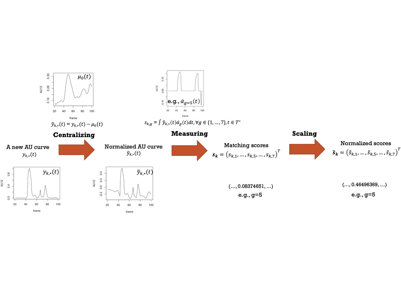
After the explanation of functional linear regressions and test methods, we are able to obtain the ground mean functions and the additional group-wise functions revealing the latent group effects on variable curves. Most importantly, we can detect the time zones where the additional effects impact significantly in statistical sense. To further examine the efficiency of the information, a natural attempt would be to apply a post hoc analysis: do classifications using the knowledge obtained and check the correctness. Before the classification, four steps are needed in our framework to project the input functions into normalized scores in lower dimensions:

• •

  First, centralize the input evolution by subtracting the estimated mean function for each sample $k$ on variable $d$.

  $$\tilde{y}_{d,k}(t)=y_{d,k}(t)-\mu_{d,0}(t)$$

• •

  Secondly, use the centralized evolution to make inner product with $G$ estimated addtional group-wise functions (also called kernels for simplicity) in turn, and thus the evolution function is projected to a vector space with $G$ dimensions. Let $S_{g,d,k}$ represent the score of group $g$ on variable $d$ in sample $k$:

  $$S_{g,d,k}=(\tilde{y}_{d,k}(t),\hat{\alpha}_{g,d}(t))=\int_{0}^{T}w_{g,d}\tilde{y}_{d,k}(t)\hat{\alpha}_{g,d}(t)dt=\int_{I}w_{g,d}\tilde{y}_{d,k}(t)\hat{\alpha}_{g,d}(t)dt,$$

  where $I$ represents the union of relevant intervals, and $w_{g,d}$ is the weights in the integral process, constant in time.

• •

  Furthermore, normalize the scores across all groups and variables from one sample $k$, so that $\tilde{S}_{g,d,k}\in[0,1]$, in order to keep the relative rate/percentage across groups.

  • –

    If $S_{g,d,k}<0$ for some $g$, move them to positive numbers by subtracting the minimum ($min\{0,min_{g}S_{g,d,k}\}$).

  • –

    Then, rescale them to be smaller than $1$ across groupss.

    $$\tilde{S}_{g,d,k}=\frac{S_{g,d,k}-min\{0,min_{g}S_{g,d,k}\}}{\sum\limits_{g=1}^{G}[S_{g,d,k}-min\{0,min_{g}S_{g,d,k}\}]}.$$

  In this way $\tilde{S}_{g,d,k}$ represents the probability that variable $d$ in sample $k$ behaves as in (has been generated by) group $g$. If the sample $k$ that we are considering is labeled with $g$, more importance is given to the variables that assign a highest probability $\tilde{S}_{g,d,k}$ to the group $g$.

• •

  Finally, combine the scores across variables for sample $k$ (labeled with $g$) by a linear convex combination with the trained weights $r_{l,g}$, such that, if the label of sample $k$ is $g$, then $S_{g,k}$ is the maximum score.

  $$S_{g,k}^{comb}=r_{1,g}\tilde{S}_{g,1,k}+r_{2,g}\tilde{S}_{g,2,k}+\dots+r_{L,g}\tilde{S}_{g,L,k},$$

  with $r_{l,g}\in[0,1]$ and $\sum\limits_{l=1}^{L}r_{l,g}=1$. For sample $k$, $[S_{1,k},S_{2,k},\dots,S_{8,k}]$ contains the scores of all groups under study, and all the elements of this vector fall in region $[0,1]$.

For classification based on scores, we apply SVM method on scores $[S_{1,k},S_{2,k},\dots,S_{G,k}]$ to classify the samples and examine the kernels efficiency. A further study on the classification methods is important but is skippped here for space saving because the classification is not the focus of this paper, although we will explore further in next study.

Assume that each curve $y_{g,d,k}(d\in\{1,\dots,D\}$ for $k$-th video can be expressed as a linear combination of basis functions $\Theta(t)=(\theta_{1}(t),\dots,\theta_{q}(t),\dots,\theta_{Q}(t))^{T}$. We define $J_{\theta\theta}$ to represent the inner product of each pair of functional basis.

Similarly, the coefficient function $\mathbf{\beta}=[\beta_{1}(t),\dots,\beta_{D}(t)]^{T}$ can be decomposed with the same functional basis in the following way

Consider that in multivariate linear regression setting

by substituting the functional curves with coefficient matrix and functional basis, we have

Notice that $\mathbf{B}$ is the coefficient that we want to estimate. Here by applying least square method on $R^{GDK\times T}$ space, we have

Let $J(\mathbf{B})=\mathbf{0}$, we can derive that

together with

References

- [1] José Ramón Berrendero, Ana Justel, and Marcela Svarc. Principal components for multivariate functional data. Computational Statistics & Data Analysis, 55(9):2619–2634, 2011.
- [2] A.J. Fridlund. Human facial expression: An evolutionary view. Academic Press, 2014.
- [3] Julien Jacques and Cristian Preda. Clustering multivariate functional data. In COMPSTAT 2012, pages 353–366, 2012.
- [4] J. Ramsay and B.W. Silverman. Functional data analysis. Springer, 1997.
- [5] S. Ullah and F. F. Caroline. Applications of functional data analysis: A systematic review. BMC medical research methodology, 2013.
- [6] J. Wrobel. Register: Registration for exponential family functional data. Journal of Open Source Software, 3(22):557, 2018.
- [7] J. Wrobel, V. Zipunnikov, J. Schrack, and J. Goldsmith. Registration for exponential family functional data. Biometrics, 75(1):48–57, 2019.