Power Allocation for IRS-aided Two-way Decode-and-Forward Relay Wireless Network

There are many thorny problems in communication networks, such as the propagation loss and multi path fading, which seriously deteriorate the communication performance [1]. With the ability to intelligently adjust the propagation environment, helpful multi path can be created by intelligent reflecting surface (IRS) for coverage extension. IRS has become an emerging technology with competitive advantages over the existing technologies [2]. IRS consists of cost-effective, low-power, and passive reflecting units, which reflect the signal independently to achieve passive beamforming for signal enhancement, spectral and energy efficiency improvement [3, 4]. IRS has been widely applied to different application scenarios, e.g., physical layer security [5], simultaneous wireless information and power transfer (SWIPT) [6], [7], mobile edge computing [8], and covert communication [9].

Due to the fact that IRS reflects signal with low-power consumption, which can be regarded as a passive relay. While the conventional relay is an active device with strong signal processing capability to amplify and forward (AF), decode and forward (DF) signal. Its high hardware cost and high-power consumption are inconsistent with our low-energy-consumption communication demand.

How to make full use of the advantages of IRS and relay to serve the wireless communication network is crucial, which has already attracted extensive attention from both academia and industry [10, 11, 12, 13]. In [10], an IRS-aided DF relay network was considered. To optimize the beamforming at relay station (RS) and phase at IRS, three methods of maximizing receive power, i.e., using alternately iterative structure, null-space projection based plus maximum ratio combining (MRC) and IRS element selection based plus MRC, were respectively proposed for rate improvement and coverage extension. For normal communication between end users in [11], a two-way AF relay network assisted by two IRSs was proposed, where alternatively optimizing phase at the two IRSs to maximize sum rate. It demonstrated that the efficiency and sum rate performance surpass that of only relay-aided system. [12] presented cooperative relay networks with IRS, where reflection amplitudes changes with the discrete phase. A deep reinforcement learning (DRL) scheme with low complexity was proposed to optimize relay selection and IRS reflection coefficient. It was shown that DRL outperformed random relay selection. In [13], the authors investigated an IRS-aided two-way AF relay network, where phase was solved by signal-to-noise ratio (SNR)-upper-bound-maximization or genetic-SNR-maximization and beamforming was achieved by optimizing beamforming or maximum-ratio beamforming. It demonstrated the proposed algorithms evidently performed better than random phase.

However, all the above literature focused on the optimization of beamforming at RS and phase at IRS, but did not consider power allocation (PA) between users and RS. PA is an efficient way to improve the sum rate, which plays an important role in sum rate. As far as we know, there is little research work on the PA of IRS-aided two-way DF relay network. This motivates us to pay attention to the PA under the total power constraint. Our main contributions are summarized as follows:

1. 1.

   To improve the sum rate performance of an IRS-aided two-way DF relay network, a PA strategy of maximizing sum rate (Max-SR) method is proposed to optimize the PA factors of two users and RS. Since the constraints are non-convex, the upper bound of the product of two PA factors and the first-order Taylor approximation of quadratic of PA factor are derived, so that the constraints can be converted into convex. The simulation results prove that the proposed Max-SR method can harvest up to 13.8% sum rate gain over equal power allocation (EPA) method.

2. 2.

   To achieve a higher sum rate, two high-performance schemes, namely maximizing minimum sum rate (Max-Min-SR) and maximizing sum rate with rate constraint (Max-SR-RC), are presented. In Max-Min-SR method, all the constraints are convex with few converted operations. In Max-SR-RC method, the first-order Taylor approximation is also applied to constraint transformation. Simulation results show that the best method among the proposed three methods and EPA is Max-SR-RC, which achieves at least 10% rate gain. Followed by Max-Min-SR method, the sum rate gain harvested is up to 15.4%.

The remainder of this paper is organized as follows. In Section II, an IRS-aided two-way DF relay network is described. In Section III, three high-performance schemes for a better sum rate performance of the proposed network is demonstrated. Simulation results are presented in Section IV, and conclusions are drawn in Section V.

Notation: Scalars, vectors and matrices are respectively represented by letters of lower case, bold lower case, and bold upper case. $(\cdot)^{T}$ and $(\cdot)^{H}$ stand for transpose and conjugate transpose, respectively. $\mathbb{E}\{\cdot\}$ and $\|\cdot\|$ denote expectation operation and 2-norm, respectively. The sign $\textbf{I}_{M}$ is the $M\times M$ identity matrix, and $\oplus$ represents exclusive or operation of two decoded symbols.

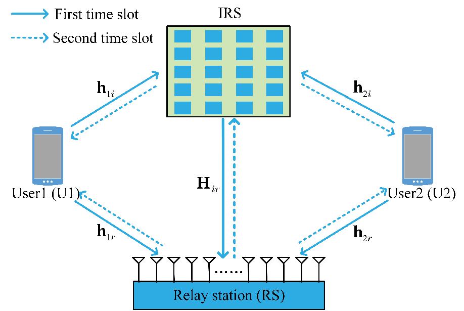
As shown in Fig. 1, we consider an IRS-aided two-way relay network. The network comprises a half-duplex two-way DF RS with $M$ transmit antennas, an IRS with $N$ reflecting elements, and two single-antenna users. Two users are respectively denoted by $U_{1}$ and $U_{2}$, which mutually exchange information with the help of IRS and RS. Due to path loss, the power of signals reflected by the IRS twice or more are such weak that they can be ignored. In the first time slot, the received signal at RS can be expressed as

where $x_{1}$ and $x_{2}$ are the independent transmit signal from $U_{1}$ and $U_{2}$, respectively. $P$ is the total transmission power and limited, $\beta_{1}$ and $\beta_{2}$ are the power allocation parameters of $U_{1}$ and $U_{2}$. $\mathbb{E}\{x_{1}^{H}{x_{1}}\}=1$ and $\mathbb{E}\{x_{2}^{H}{x_{2}}\}=1$. Without loss of generality, we assume a Rayleigh fading environment [14]. Let $\textbf{h}_{1r}$$\in\mathbb{C}^{M\times 1}$, $\textbf{H}_{ir}\in\mathbb{C}^{M\times N}$ and $\textbf{h}_{1i}\in\mathbb{C}^{N\times 1}$ represent the channels from $U_{1}$ to RS, from IRS to RS, and from $U_{1}$ to IRS, $\textbf{h}_{2r}$$\in\mathbb{C}^{M\times 1}$ and $\textbf{h}_{2i}\in\mathbb{C}^{N\times 1}$ represent the channels from $U_{2}$ to RS and from $U_{2}$ to IRS. $\bm{\Theta}_{1}$ is the diagonal reflection-coefficient matrix of IRS, which is denoted as $\bm{\Theta}_{1}=\text{diag}(e^{j\theta_{1}},\cdots,e^{j\theta_{N}})$, $\theta_{i}\in(0,{2\pi}]$ is the phase shift of the $i$th element. $\textbf{n}_{r}\in\mathbb{C}^{M\times 1}$ is the additive white Gaussian noise (AWGN) with distribution $\textbf{n}_{r}\sim\mathcal{CN}(0,\sigma_{r}^{2}{\bf I}_{M})$. Considering $x_{2}$ as unknown interference, RS first decodes $x_{1}$ to $\widetilde{x}_{1}$. Then the contribution of $x_{1}$ can be eliminated from (II), and $x_{2}$ can be decoded to $\widetilde{x}_{2}$.

In the second time slot, network coding is employed for $\widetilde{x}_{1}$ and $\widetilde{x}_{2}$, and combining them into a new signal, which is represented as

Each user decodes ${x}_{r}$ to $\widetilde{x}_{r}$, and rebuild the symbol sent by the other user (i.e, $\overline{x}_{2}=\widetilde{x}_{r}\oplus{x}_{1}$ or $\overline{x}_{1}=\widetilde{x}_{r}\oplus{x}_{2}$). It is assumed that the channel reciprocity holds, i.e., the channels in the second-time slot can be represented as the conjugate transpose of the channels in the first-time slot. After self-interference cancellation, the received signal at $U_{1}$ is written by

where $\overline{\textbf{x}}_{2}=\overline{x}_{2}[1,1,\cdot\cdot\cdot,1]^{T}\in\mathbb{C}^{M\times 1}$. Similarly, the received signal at $U_{2}$ is given by

where $\overline{\textbf{x}}_{1}=\overline{x}_{1}[1,1,\cdot\cdot\cdot,1]^{T}\in\mathbb{C}^{M\times 1}$, $\beta_{3}$ is the power allocation parameter of RS, the diagonal reflection-coefficient matrix of IRS is represented as ${\bm{\Theta}}_{2}=\text{diag}\left(e^{j{\theta_{21}}},\cdots,e^{j{\theta_{2N}}}\right)$, ${\theta_{2i}}\in\left(0\right.,\left.{2\pi}\right]$ is the phase shift of the $i$th element. $n_{1}$ and $n_{2}$ are the AWGN with distribution $n_{1}\sim\mathcal{CN}\left(0,{\sigma_{1}^{2}}\right)$ and $n_{2}\sim\mathcal{CN}\left(0,{\sigma_{2}^{2}}\right)$, respectively. The achievable rate of $U_{1}$-RS-$U_{2}$ link can be expressed as follows

where $R_{1ir}$ and $R_{ri2}$ are the rates of $U_{1}$-RS and RS-$U_{2}$ link, respectively,

and

Similarly, the achievable rate of $U_{2}$-RS-$U_{1}$ link can be represented as follows

where $R_{2ir}$ and $R_{ri1}$ are the rates of $U_{2}$-RS and RS-$U_{1}$ link, respectively,

and

The achievable multiple access channel (MAC) rate of $U_{1}$-RS and $U_{2}$-RS can be represented as follows

Therefore, the achievable sum rate of the proposed system is defined as follows

In this section, we focus on the investigation of PA methods to maximize $R$, and the optimization problem is casted as

where $\bm{\Theta}_{1}$ and $\bm{\Theta}_{2}$ are obtained by maximizing the sum rate via general power iterative in [15]. In this paper, $\bm{\Theta}_{1}$ and $\bm{\Theta}_{2}$ refer directly to [15]. The above optimization problem is simplified to

To solve the optimization problem, three PA schemes are proposed, which are Max-SR, Max-Min-SR and Max-SR-RC, respectively, and the related details are as follow.

In this section, numerical simulations are performed to evaluate and compare the sum rate performance between the proposed three methods and EPA method. Moreover, it is assumed that $U_{1}$, $U_{2}$, IRS and RS are located in three-dimensional (3D) space, the positions of $U_{1}$, $U_{2}$, IRS and RS are given as (0, 0, 0), (0, 100m, 0), ($-$10m, 50m, 20m) and (10m, 50m, 10m), respectively. We take a more realistic environment into account, and assume that all channels follow large-scale fading, which contains shadow fading. The path loss model is $PL(d)=PL_{0}-10{\alpha}\text{log}_{10}(\frac{d}{d_{0}})-X_{\sigma}$, where $PL_{0}=-20\text{log}_{10}(\frac{4{\pi}d_{0}}{\lambda})$ is the path loss at the reference distance $d_{0}$, $\lambda$ is wavelength, $\alpha$ is the path loss exponent, and $X_{\sigma}$ is a Gaussian random shadow variable with distribution $X_{\sigma}\sim\mathcal{CN}(0,\sigma^{2})$. The path loss exponents associated with IRS are 2.1, those of $U_{1}$-RS and $U_{2}$-RS links are 2.3. The remaining system parameters are set as follows: $f_{c}=$ 1.5GHz, $\sigma_{1}^{2}=\sigma_{2}^{2}=\sigma_{r}^{2}=-$80dBm.

Fig. 2 illustrates the achievable sum rate of Max-SR-RC method versus $\mu$ with different total power: $P=\{$0dBm, 10dBm, 20dBm, 30dBm$\}$. It can be seen that as $\mu$ increases, the sum rate performance gradually increases. Until $\mu\geq$ 3, the achievable sum rate tends to be stable. For convenience, $\mu$ is defined as 3.

Fig. 3 depicts the histogram of achievable sum rate versus total power with $M=$ 4, $N=$ 16 and $\sigma=$ 3dB. It can be seen that the proposed three methods perform better than EPA method. For instance, when total power equals 10dBm, the proposed worst method, Max-SR, can harvest up to 5.3% rate gain over EPA method. The best method, Max-SR-RC, approximately has a 37.9% rate gain over EPA method.

Fig. 4 shows the corresponding histogram of achievable sum rate versus $\sigma$ with total power $=$ 40dBm, $M=$ 4 and $N=$ 16. When $\sigma=$ 5dB, it can be observed that the achievable sum rate performance improvements over EPA method are 13.8%, 15.4% and 45.2%, respectively. Moreover, it indicates that as $\sigma$ increases, the sum rate performance gain becomes more obvious, which is very attractive. However, greater shadowing fading is formed because of the increase of $\sigma$, which sharply deteriorates the sum rate performance.

In this paper, in order to improve the achievable sum rate of an IRS-aided two-way DF relay wireless network, three high-performance PA schemes, namely Max-SR, Max-Min-SR and Max-SR-RC, were proposed. Simulation results showed that the proposed three methods can harvest better rate gain over EPA method in terms of sum rate performance. Because of excellent rate performance, the proposed Max-SR-RC method is very attractive. Additionally, the rate increases with total power, while decreases with $\sigma$.

References

- [1] X. Cheng, Y. Lin, W. Shi, J. Li, C. Pan, F. Shu, Y. Wu, and J. Wang, “Joint optimization for RIS-assisted wireless communications: From physical and electromagnetic perspectives,” IEEE Trans. Commun., vol. 70, no. 1, pp. 606–620, Jan. 2022.
- [2] Q. Wu and R. Zhang, “Towards smart and reconfigurable environment: Intelligent reflecting surface aided wireless network,” IEEE Commun. Mag., vol. 58, no. 1, pp. 106–112, Jan. 2020.
- [3] W. Tang, J. Y. Dai, M. Z. Chen, K.-K. Wong, X. Li, X. Zhao, S. Jin, Q. Cheng, and T. J. Cui, “Mimo transmission through reconfigurable intelligent surface: System design, analysis, and implementation,” IEEE J. Sel. Areas Commun., vol. 38, no. 11, pp. 2683–2699, Nov. 2020.
- [4] Y. Wu, F. Zhou, W. Wu, Q. Wu, R. Q. Hu, and K. K. Wong, “Multi-objective optimization for spectrum and energy efficiency tradeoff in IRS-assisted CRNs with NOMA,” IEEE Trans. Wireless Commun., pp. 1–1, 2022.
- [5] F. Shu, Y. Teng, J. Li, M. Huang, W. Shi, J. Li, Y. Wu, and J. Wang, “Enhanced secrecy rate maximization for directional modulation networks via IRS,” IEEE Trans. Commun., vol. 69, no. 12, pp. 8388–8401, Dec. 2021.
- [6] W. Shi, X. Zhou, G. Xia, Y. Wu, F. Shu, and J. Wang, “Enhanced secure wireless information and power transfer via intelligent reflecting surface,” IEEE Commun. Lett., vol. 70, no. 2, pp. 1084–1088, Apr. 2020.
- [7] C. Pan, H. Ren, K. Wang, M. Elkashlan, A. Nallanathan, J. Wang, and L. Hanzo, “Intelligent reflecting surface aided mimo broadcasting for simultaneous wireless information and power transfer,” IEEE J. Sel. Areas Commun., vol. 38, no. 8, pp. 1719–1734, Aug. 2020.
- [8] T. Bai, C. Pan, H. Ren, Y. Deng, M. Elkashlan, and A. Nallanathan, “Resource allocation for intelligent reflecting surface aided wireless powered mobile edge computing in OFDM systems,” IEEE Trans. Wireless Commun., vol. 20, no. 8, pp. 5389–5407, Aug. 2021.
- [9] X. Zhou, S. Yan, Q. Wu, F. Shu, and D. Ng, “Intelligent reflecting surface (IRS)-aided covert wireless communications with delay constraint,” IEEE Trans. Wireless Commun., vol. 21, no. 1, pp. 532–547, Jan. 2022.
- [10] X. Wang, F. Shu, W. Shi, X. Liang, R. Dong, J. Li, and J. Wang, “Beamforming design for IRS-aided decode-and-forward relay wireless network,” IEEE Trans. Green Commun. Netw., vol. 6, no. 1, pp. 198–207, Mar. 2022.
- [11] Y. Tao, Q. Li, and X. Ge, “Sum rate optimization for IRS-aided two-way af relay systems,” in 2021 IEEE/CIC Int. Conf. Commun. in China (ICCC), 2021, pp. 823–828.
- [12] C. Huang, G. Chen, Y. Gong, M. Wen, and J. A. Chambers, “Deep reinforcement learning-based relay selection in intelligent reflecting surface assisted cooperative networks,” IEEE Wireless Commun. Lett., vol. 10, no. 5, pp. 1036–1040, May 2021.
- [13] J. Wang, Y.-C. Liang, J. Joung, X. Yuan, and X. Wang, “Joint beamforming and reconfigurable intelligent surface design for two-way relay networks,” IEEE Trans. Commun., vol. 69, no. 8, pp. 5620–5633, Aug. 2021.
- [14] H. Zhu and J. Wang, “Chunk-based resource allocation in ofdma systems - part i: chunk allocation,” IEEE Transactions on Communications, vol. 57, no. 9, pp. 2734–2744, Sept. 2009.
- [15] P. Zhang, X. Wang, S. Feng, Z. Sun, F. Shu, and J. Wang, “Phase optimization for massive irs-aided two-way relay network,” 2022. [Online]. Available: http://arxiv.org/abs/2203.09185.