Manifold Principle Component Analysis for Large-Dimensional Matrix Elliptical Factor Model
Abstract
Matrix factor model has been growing popular in scientific fields such as econometrics, which serves as a two-way dimension reduction tool for matrix sequences. In this article, we for the first time propose the matrix elliptical factor model, which can better depict the possible heavy-tailed property of matrix-valued data especially in finance. Manifold Principle Component Analysis (MPCA) is for the first time introduced to estimate the row/column loading spaces. MPCA first performs Singular Value Decomposition (SVD) for each “local” matrix observation and then averages the local estimated spaces across all observations, while the existing ones such as 2-dimensional PCA first integrates data across observations and then does eigenvalue decomposition of the sample covariance matrices. We propose two versions of MPCA algorithms to estimate the factor loading matrices robustly, without any moment constraints on the factors and the idiosyncratic errors. Theoretical convergence rates of the corresponding estimators of the factor loading matrices, factor score matrices and common components matrices are derived under mild conditions. We also propose robust estimators of the row/column factor numbers based on the eigenvalue-ratio idea, which are proven to be consistent. Numerical studies and real example on financial returns data check the flexibility of our model and the validity of our MPCA methods.
Keywords: Factor Model; Grassmann manifold; Matrix elliptical distribution; Principle component analysis.
1 Introduction
Factor models have been a classical dimension reduction tool in statistics, which is popular for its ability to summarize information in large data sets. More importantly, factor models characterize many economic problems, e.g., the Arbitrage Pricing Theory of Ross 1976. In the last two decades large-dimensional approximate factor model is growing popular as we embrace the big data era where more and more variables are recorded and stored, see the seminal work by Bai and Ng 2002 and Stock and Watson 2002, and some representative work by Bai 2003,Onatski 2009, Ahn and Horenstein 2013, Fan et al. 2013, Bai and Li 2012, Bai and Li 2016 and Trapani 2018. The aforementioned papers all require the fourth moments (or even higher moments) of factors and idiosyncratic errors exist, which may be constrictive in research areas such as finance. He et al. 2022 for the first time propose a Robust Two Step (RTS) procedure to do factor analysis without any moment constraints, under the framework of elliptical distributions, see also the endeavors by Yu et al. 2019, He et al. 2020 and Chen et al. 2021a.
The modern data collected are usually well-structured in a matrix form, such as time list of tables recording several macroeconomic variables across a number of countries; a series of customers’ ratings on a large number of items in an online platform, see Chen and Fan 2021 for further examples of well-structured matrix observations. In the last few years, matrix factor model has drawn growing attention as an important two-way dimension reduction tool for matrix sequences. Wang et al. 2019 for the first time proposed the following matrix factor model:
| (1.1) |
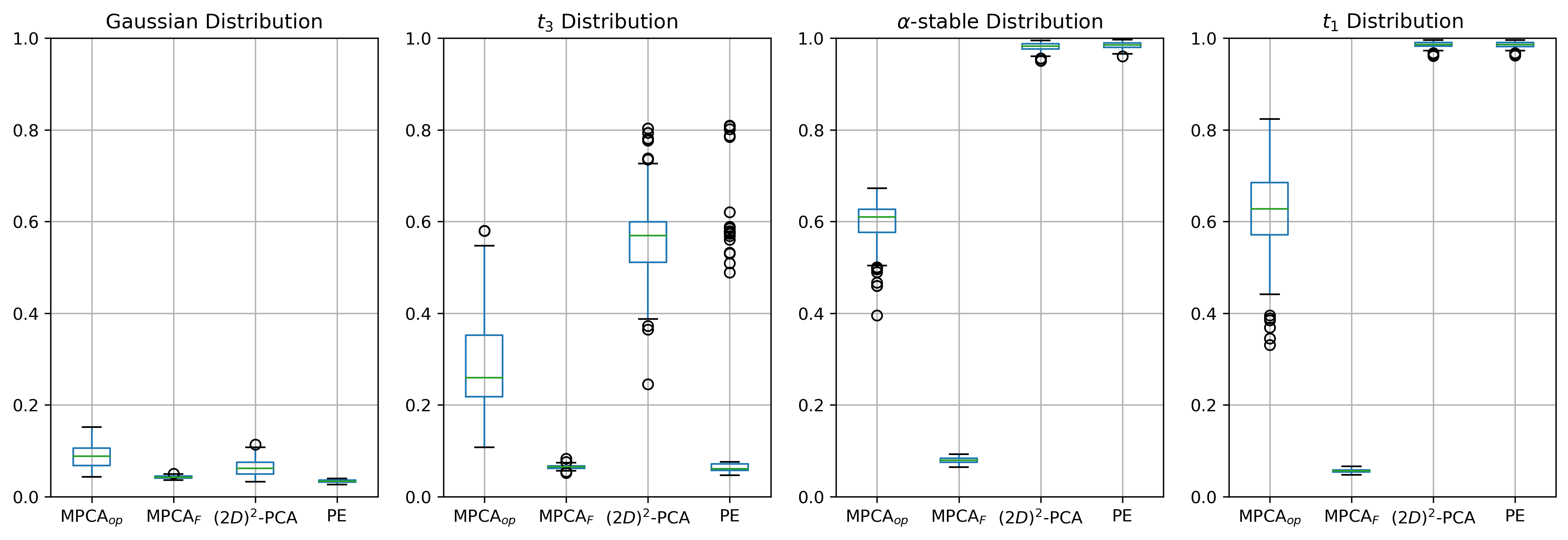
where are matrix observations of dimension , is the row factor loading matrix exploiting the variations of across the rows, is the column factor loading matrix reflecting the differences across the columns of , is the common factor matrix for all cells in and is the idiosyncratic components. A naive way to do factor analysis for matrix observations is to first vectorize the data , and then to adopt the classical well-developed vector factor models techniques. However, when data genuinely have a matrix factor structure as in (1.1), this naive approach would lead to sub-optimal inference (Chen and Fan 2021; He et al. 2021c). Two different types of matrix factor model assumptions are adopted in the existing literature. One type of models assumes that the factors accommodate all dynamics, making the idiosyncratic noise “white” with no autocorrelation but allowing substantial contemporary cross-correlation among the error process, and the estimation of the loading space is done by an eigen-analysis of the nonzero lag autocovariance matrices, see for example Wang et al. 2019. The other type of models assumes that a common factor must have impact on almost all (defined asymptotically) of the matrix time series, but allows the idiosyncratic noise to have weak cross-correlations and weak autocorrelations, and principle component analysis (PCA) of the sample covariance matrix is typically used to estimate the spaces spanned by the row/column loading matrices, see for example Chen and Fan 2021; Yu et al. 2021; He et al. 2021a. As far as we know, all the existing work on matrix factor model assumes that the fourth moments (or even higher moments) of factors and idiosyncratic errors exist, which could be restrictive in real applications such as in finance. Figure 1 depicts the boxplots of the row factor loading estimation errors based on 100 replications, from which we can see that the -PCA by Zhang and Zhou 2005 and the Projection Estimation (PE) method by Yu et al. 2021 results in bigger biases and higher dispersions as the distribution tails become heavier.
In the current work, we for the first time propose a freshly new and flexible model, named as the Matrix Elliptical Factor Model (MEFM), which assumes that the factor matrix and the idiosyncratic errors matrix follow an joint Elliptical Matrix Distribution (EMD), which covers a large class of heavy-tailed matrix distributions such as matrix -distribution. To estimate the row (column) loading space () of MEFM robustly, we propose a Manifold Principle Component Analysis (MPCA) method for the first time. In essence, for each data matrix , assume that for better illustration, the MPCA first finds the best -dimensional row (column) loading space estimator (), which can be viewed as an element in the Grassmann manifold (), where the Grassmann manifold is the set of -dimensional linear subspaces of the (Ham and Lee 2008). Then MPCA looks for the “centers” of all row/column loading space estimators within their Grassmann manifolds respectively. According to the way of finding the best linear row/column space for each matrix observation, the MPCA then has two versions, and , corresponding to the optimization problem (2.2) under matrix operator norm and matrix Frobenius norm respectively. For the , the projection technique in Yu et al. 2021 happens to be taken into account, which increases the signal-to-noise ratio. Now, let us come back to Figure 1, in which we also presented the results using the and methods. It can be seen that always performs well under various distributions, and is even not sensitive to the elliptical assumption (noting that -stable distribution is not elliptical). The method also exhibits an extent of robustness, while it is inferior to the in all cases. This indicates that for matrix factor model, the projection technique is always preferred as it can increase the signal-to-noise ratio.
To do matrix factor analysis, the first step is to determine the pair of factor numbers. As for the Elliptical Matrix Factor Model (MFM), both the row and column factor numbers should be predetermined. Wang et al. 2019 proposed to estimate the pair of factor numbers by the ratios of consecutive eigenvalues of auto-covariance matrices; Chen and Fan 2021 proposed an -PCA based eigenvalue-ratio method and Yu et al. 2021 further proposed a projection-based iterative eigenvalue-ratio method, all borrowing the eigenvalue ratio idea from Ahn and Horenstein 2013. He et al. 2021a is the only work that determines the pair of factor numbers from the perspective of sequential hypothesis testing. In this article we also propose similar eigenvalue ratio methods based on the MPCA approach. The proposed estimators of the pair of factor numbers are proven to be consistent under mild conditions and performs much better than the existing ones when the matrix-valued data are heavy-tailed shown in the simulation study.
The contributions of the current work lie in the following aspects. Firstly, we for the first time propose a flexible matrix elliptical factor model for matrix observations which is adaptive to their tail properties. Secondly, to estimate the loading spaces of MEFM robustly, we for the first time introduce a freshly new principle component analysis method, named as the Manifold Principle Component Analysis (MPCA), which is computationally efficient and easy to implement. The MPCA is completely different from the traditional PCAs (e.g., the -PCA by Chen and Fan 2021 and -PCA by Zhang and Zhou 2005) method in the sense that MPCA first performs Singular Value Decomposition (SVD) for each “local” matrix observation and then integrates/averages the local spaces, while the traditional PCAs first integrates the matrix observations and then finds the principle eigenvectors of the sample covariance matrices. Clearly, the MPCA would show great computational advantage especially in online updating problems. Thirdly, the theoretical guarantee of MPCA relies heavily on the properties of the expected projection matrices, which has not aroused much attention in existing literatures. We show that the expected projection matrices contain adequate subspace information, which is of independent interest. At last, the theoretical analysis shows that the proposed MPCA estimators are consistent without any moment constraints on the underlying distributions of the factors and the idiosyncratic errors, which generalize the methods’ applicability to heavy-tailed datasets such as financial returns.
The remainder of the article is organized as follows. In Section 2, we first introduce the proposed matrix elliptical factor model. Then we introduce the Manifold Principle Component Analysis (MPCA) method, and take the special degenerated case to illustrate the intuition of its robustness. At last we introduce the best subspace approximation for each matrix observation under both the matrix operator norm and the matrix Frobenius norm, by which we further propose the two versions of MPCA algorithms. In Section 3, we investigate the theoretical properties of the estimators by MPCA, including the factor loadings, factor scores and common components matrices. In Section 4, we further discuss the selection of the pair of factor numbers and propose two procedures based on the eigenvalue ratio idea. In section 5, we conduct thorough numerical studies to illustrate the advantages/robustness of the MPCA method and the corresponding eigenvalue-ratio factor number estimation methods over the state-of-the-art methods. In Section 6, we analyze a financial returns dataset to illustrate the practical value of the proposed methods. We conclude the article and discuss the limitation of the current work and possible future research directions in Section 7. The proofs of the main theorems and additional details are collected in the supplementary materials.
To end this section, we introduce some notations throughout the study. For matrix , and represent the operator norm and Frobenius norm, denotes the trace of , and means vectorization, denotes the -th largest singular value of . Moreover, if is symmetric, denotes the -th largest eigenvalue of , and let be the -th eigengap. For vector , denote -norm as . The notation means identically distributed. The is for convergence to zero in probability and is for stochastic boundedness. For two random series and , means that , and means that . The notation means that and . denotes the space of matrices with orthogonal columns. means rounding to the nearest integer. The constants and may not be identical in different lines.
2 Methodology
2.1 Matrix Elliptical Factor Model
For matrix-variate sequences , the centered matrix factor model is introduced by Wang et al. 2019 as follows:
where is the row factor loading matrix, is the column factor loading matrix, is the common factor matrix and is the idiosyncratic component with and . This model is suited for well-structured tables of macroeconomic indicators, financial characteristics, and frames of pictures etc. In this paper, we are interested in recovering the loading spaces and . Without loss of generality, we assume and . The projection matrices onto and are then naturally and .
Prior to the introduction of Matrix Elliptical Factor Model (MEFM), we first take a look at matrix elliptical distributions. A random matrix of size is matrix elliptical distributed if its characteristic function has the form with : : , : , : , , and . This distribution is denoted by , see Gupta and Nagar 2018 for details. An important observation given in Gupta and Varga 1994 shows that for , , the random matrix if and only if:
where : and is uniformly distributed on the unit sphere in , is a nonnegative random variable independent of , and are rank factorizations of and . The matrix Gaussian distributions and matrix -distributions belong to the class of matrix elliptical distributions. In the article, in the definition of MEFM, we assume the factor and noise are from joint matrix elliptical distribution as in He et al. 2022, which is:
| (2.1) |
where is a -dimensional isotropic Gaussian vector, while is a positive random variable independent of . It is sometimes more convenient to separate the joint model into:
with positive-definite transformation matrices of size , of size , of size and of size . is a random matrix by taking the leading elements of , while of size consists of all the elements left. It is not hard to verify that and are matrix elliptical distributed, since is independent of both and .
Remark 2.1.
Assuming the joint matrix elliptical distribution of and is to ensure distribution-free signal-to-noise conditions. For example, if has i.i.d. standard Gaussian elements, then . On the other hand, if has i.i.d. elements, then . Assuming joint matrix elliptical distribution ensures simplicity, otherwise, the signal-to-noise conditions are distribution-dependent, and higher signal-to-noise ratio is naturally required for heavier-tailed noise case. See the same joint (vector) elliptical distribution assumption in Fan et al. 2018; He et al. 2022.
2.2 Manifold Principle Component Analysis
In this section, we introduce our Manifold Principle Component Analysis (MPCA) method for MEFM estimation. As a simple heuristic argument to see the robustness of MPCA, first consider and then the matrix factor model degenerates to the vector case. The classical vector factor model would be written as:
where is the observed vector, is the loading matrix, is the latent factor vector and is the noise vector. The classical PCA seeks the leading eigenvectors of the sample covariance matrix , which is easily influenced by outliers, as those with larger norm naturally have larger influence on .
It would be more robust to treat all equally, in a sense that each provides the same amount of subspace information. The Manifold PCA (MPCA) first finds the best subspace estimation for each , which is the first eigenvector of the rank one matrix . Then it seeks the “center” of all , which would be the leading eigenvectors of the average projection matrix . It is exactly a distance-weighted sample covariance, namely:
Such degeneration towards vector factor model provides some basic insights for the robustness of our MPCA methods against heavy-tailed noises. If the data set is augmented to , our method is then equivalent to calculating the leading eigenvectors of the multivariate Kendall’s matrix, which is also valid without moment conditions, see He et al. 2022 for details.
We then introduce the MPCA methods for matrix variate data. Assume first , for each data matrix , we give the best linear row/column space estimator for , denoted by orthogonal matrices and respectively, which are the representatives of their own equivalent classes on the Grassmann manifolds and . Then MPCA finds the “centers” of all and within their Grassmann manifolds respectively.
In the following section, we will show that for each , the best linear subspace estimator and are the leading eigenvectors of and with respect to operator norm loss in (2.2) below. Similarly, and are leading eigenvectors of and under Frobenius norm loss if and are given respectively.
Then, for given linear space estimators and for each , it is natural to find their “centers” on the Grassmann manifolds and as the final estimators. However, Grassmann manifolds admit highly non-linear structures and direct sample averaging is not admissible. Fortunately, we show that the leading eigenvectors of the average projection matrices and , denoted by and , could serve as the representatives of the Manifolds.
Remark 2.2.
Although such manifold center intuition seems vivid, we have to be more careful with those degenerated cases where the best linear subspace approximation for each single matrix data is of lower dimensional than expected. For instance, if the factor matrix is of dimension with , and we wish to find a -dimensional subspace . The signal part would be of rank , so it would be more natural to set as the leading left singular vectors of , instead of . The algorithm could be slightly modified and performs equally well, but the intuition of manifold “center” no longer makes sense, as each is -dimensional while the we seek is -dimensional. That is to say, we are finding the -dimensional “centered” subspace among some -dimensional subspaces, hence we adopt the term degeneration.
2.3 Best Subspace Approximations
First, consider the best subspace approximation for a single matrix data . We aim to find basis matrices and of dimension and respectively, and the compressed factor matrix such that is sufficiently close to the original . It is then natural to solve the following optimization problem for some matrix norm ,
| (2.2) |
For the Frobenius norm , it is well-known that if and are given, would simply be the projected value , see He et al. 2021b. After simple matrix manipulation, would be the leading eigenvectors of and would be the leading eigenvectors of .
For the operator norm , unfortunately, a close form solution for even if and are given is vacant. However, the optimized value has a closed form for , if the largest singular values of do not coincide so that the operator norm is differentiable, which is:
where and are respectively the largest singular values of the matrices and , defined as
We could minimize and separately. It is then straightforward that and are the leading left and right singular vectors of the matrix data . In the end, as the optimization problem is sufficiently continuous and operator norm is differentiable almost everywhere except for a zero Lebesgue measure set, the above solutions would be numerically valid.
2.4 MPCA algorithms for MEFM
In this section, we give the details of the MPCA algorithms. We first discuss the operator loss approximation case, naming this variant as . As discussed earlier, first acquires the best linear subspace approximation and for each data matrix by singular value decompositions. For non-degenerated cases namely , and would be the leading left and right singular vectors of , which are the representatives of elements on the Grassmann manifolds and respectively. Then, finds the centers by minimizing the projection metrics on Grassmann manifolds:
which is analogous to the physical notion of barycenter. Without loss of generality, we only focus on discussion of here. Denote and , then we have:
The first two terms on the right hand side are fixed, so we are actually maximizing the last term, namely . It is a classical eigenvalue problem and would be the leading eigenvectors of the average projection matrix .
As for the degenerated case where , without loss generality we assume , then and are the leading left and right singular vectors of . Solve the same optimization problem and , are still the leading , eigenvectors of the average projection matrices , respectively. It is easy to see that is exactly the same as in the non-degenerated case. As for , it is of size . It is no longer a representative of some element in , thus the manifold center intuition no longer holds. However similar geometric interpretation is still somehow valid: each corresponds to a -dimensional subspace, and with some principal angle related arguments, still gives the magnitude of deviation of -dimensional from the -dimensional . It is obvious that needs , as we are seeking for lower dimensional column and row subspaces, and the right hand side is the maximal rank of the original data matrices . The detailed procedures for is summarized in Algorithm 1.
We now discuss the Frobenius loss case, naming this variant as . Under Frobenius loss, would be the leading eigenvectors of if is given and would be the leading eigenvectors of if is given. Then takes the leading eigenvectors of the average projection matrices similarly. Note that iterative procedure is necessary as and is unavailable at the beginning. For initial value, the estimators by can be adopted as a warm start. The detailed procedures for is summarized in Algorithm 2.
3 Theoretical Results
In this section, we present the theoretical properties of the estimators by MPCA, and throughout this section, the number of factors and are treated as given. The determination of factor numbers , are left to Section 4.
3.1 Expected Projection Matrix
Prior to presenting the consistency of our MPCA estimators, we first give some intuitions on why the algorithms work. For clearer illustration, we only analyze by . Recall that the model is , while is the leading left singular vectors of . In the end, is acquired by taking the leading eigenvectors of the average projection matrix . Obviously, the algorithm relies heavily on the concentration of average projection matrix to its expected version . The algorithms could be justified as long as we show that:
- 1.
The average projection matrix converges to the expected version at a rate of .
- 2.
The leading eigenvectors of the expected version give us as desired.
As for the first part, with the help of matrix concentration inequalities in Tropp 2012, we have:
Lemma 3.1 (-Convergence).
For i.i.d. random projection matrices with dimension , for all , the following concentration inequality holds,
Although we are quite satisfied with this -consistency result for finite-dimensional matrix data, the haunting dimensional factor of matrix concentration inequalities would give exploding bounds if the dimension tends to infinity. Fortunately, in this case of random projection matrices, we are able to shrink the dimensional factor to via intrinsic dimension arguments. As remains fixed as goes to infinity, dimension-free convergence could be acquired.
As for the second part, we claim that and are invariant subspaces of the expected projection matrix if the noise is left spherical. Matrix spherical distribution can be viewed as a special case of matrix elliptical distribution. The random matrix is left spherical if , right spherical if and spherical if . If is left spherical, then , . Right spherical and spherical distributions have similar properties accordingly. Random matrices with i.i.d. centered Gaussian or elements are matrix spherically distributed, see Gupta and Nagar 2018 for details.
Lemma 3.2 (Invariant Subspaces).
For joint matrix elliptical data as in 2.1, let , where is the leading eigenvectors of . If is left spherical, then and are invariant subspaces of .
The joint matrix elliptical model here is more of a burden instead of blessing. In fact, the conclusion is more straightforward if and are independent and could be of independent interet. The combination of Lemmas 3.1 and 3.2 theoretically justifies the validity of the proposed MPCA methods: the expected projection matrix contains adequate subspace information, while the matrix concentration to it is guaranteed by the compactness of the projection matrices.
3.2 Technical Assumptions
In this section, we give some technical assumptions to establish the convergence rates of the estimators by MPCA.
Assumption A (Joint Matrix Elliptical Model).
We assume matrix elliptical factor model as:
where is a -dimensional isotropic Gaussian vector, is a positive random variable independent of , with as . It is sometimes more convenient to separate the joint model into:
with of size , of size , of size and of size . is a random matrix made by leading elements of , while of size consists of all the elements left.
Assumption B (Strong Factor Conditions).
We assume and . In addition, there exist positive constants and such that , as .
Assumption C (Regular Noise Conditions).
We assume there exist positive constants and such that , as .
The convergence relies heavily on matrix concentration results. The independence between in Assumption A could extend readily to weak dependence by matrix concentration results such as matrix Azuma inequality, see Tropp 2012, Tropp 2015 for details. Assumption B and C are standard in large-dimensional factor models. In addition, the joint matrix elliptical distribution assumption is only for the convenience of theoretical analysis, while empirical experiments show that the MPCA methods are not sensitive to the elliptical assumption.
3.3 Consistency of Manifold PCA
Theorem 3.3 (Consistency of ).
As MPCA methods rely heavily on the concentration of projection matrices, the convergence rate would be at most . It is slower than -PCA from Chen and Fan 2021 and PE from Yu et al. 2021 with the rate (or ) when estimating (or ) under strong signal conditions, which are comparable to taking each column (or row) as individual observation. The inefficiency of MPCA methods comes from the fact that by taking each projection matrix as individual observation would lose information especially when each matrix observation is of large dimensions. However, as we will see in the simulation study, MPCA performs comparably to the classical methods for Gaussian noise, while the compactness of the projection matrices ensures the good performance of MPCA even for noises without any moments. As a result, they could be potential replacements of classical methods for data with heavier-tailed noise.
For method, we further discuss how the information of column factor loading matrix would help to estimate , which is named as the projection effect in this work. Estimation of can be discussed in a similar way. Recall that for , would be the leading eigenvalues of if is given. Let for notational simplicity. We focus on the projected matrix model , and would exactly be the estimator by the MPCAop to the projected data set .
The difference with/without projection lies in the signal-to-noise ratio level. Consider the extreme case where the true value is known, for , the projection does no harm to the signal size while compressing the noise to lower-dimensional . It is then foreseeable that we could increase the signal-to-noise ratio via projection by some sufficiently close to , keeping the signal size almost unchanged. It is ensured by assuming , which is a rather mild condition.
3.4 Factor and Common Component Matrices
After the loading matrices being determined, the factor matrix can be naturally estimated by , and the common component matrix be estimated by .
Corollary 3.1 (Consistency of Factor and Common Component Matrices).
Suppose there exist orthonormal matrix and orthonormal matrix such that for and , we have and , then:
4 Determining the Factor Numbers
In the last section, the factor number is assumed to be known in advance, while in practice, the factor numbers and need to be determined. We propose a natural criterion by calculating eigenvalue-ratios (ER) of the average projection matrices, under both and . The corresponding algorithms are named as and respectively. Unlike existing eigenvalue-ratio methods based on covariance-type matrices as in Chen and Fan 2021 and Yu et al. 2021, and are clearly free of moment-constraints. For , first determine the compression rank by averaging acquired from each data matrix , that is:
where means rounding to the nearest integer. Then and are estimated by:
| (4.1) |
where is predetermined value larger than , , while , are the average projection matrices by taking the leading left and right singular vectors of each respectively.
Remark 4.1.
In fact, accurate estimation of is not necessary for , we could still get comparable results from 4.1 even if . However, since each data matrix contains at most -dimensional subspace information, pre-estimation of could stabilize the algorithm. Once has been correctly estimated, would be exactly in MPCAop. Further analysis in supplementary materials ensures that , while as under Assumption A to C, which theoretically justifies .
Theorem 4.2 (Consistency of estimators).
Similarly, we could use the average projection matrices from to increase accuracy. Now that estimating requires information of , and estimating requires information of , iterations are naturally needed, and the result from estimators could be used as a warm start.
Theoretical analysis of is challenging due to the iteration procedure, thankfully the initial step taken from has already been consistent under Assumption A to C. As shown in simulations, benefits from the same projection technique as in and turns out to be more accurate than in finite-sample performances.
5 Simulation Results
In this section, we investigate the finite-sample performances of MPCA algorithms by generating synthetic datasets. The observed data matrices are generated as from moderate noise regime, by rescaling signal and noise to the same scale.
5.1 Data Generation
To generate observations from the model , , we set , draw the entries of and from independent standard Gaussian distribution, and let:
where and the elements of are generated by independent standard centered Gaussian, , skewed- and -stable distributions. The rescaling constant is to get comparable signal and noise level. In fact, if consists of independent standard centered Gaussian random variables, the signal part while , thus by setting we get comparable signal and noise level. On the other hand, if consists of independent random variables, it holds , then we need to set .
The pair of dimensions are chosen from the set , the sample size is set to be and , are set to be matrices with ones on the diagonal, and , on the off-diagonal respectively. In addition, the parameters and control temporal correlation and are set as , while is the noise scaling constant chosen from . We only show the cases with in this section, and the rest are left to the supplementary materials. Elements of are drawn independently from standard Gaussian, , , -stable distribution (, skewness parameter ), and skewed- distribution (standard deviation , skewness parameter ) respectively, while we set for distribution and for the rest distributions. We generate -stable distribution by Python package scipy.stats, and skewed- distribution by Python package sstudentt. All simulation results reported here are based on 100 replications.
5.2 Estimation of Loading Spaces
We first compare the performances of MPCA algorithms with those of -PCA by Zhang and Zhou 2005 and PE method by Yu et al. 2021in terms of estimating loading spaces. In fact, -PCA is equivalent to -PCA from Chen and Fan 2021 with , whose empirical performances corresponding to are comparable as shown in Yu et al. 2021. To measure the difference between the estimated and the true loading , we used the scaled projection metric as in Yu et al. 2021, which is defined as:
so it is straightforward that is always between (corresponding to ) and (corresponding to and are orthogonal). can be defined similarly.
| Distribution | Evaluation | MPCAop | MPCAF | -PCA | PE | ||
| Gaussian | 20 | 20 | (0.3024,0.1272) | (0.1154,0.0233) | (0.2007,0.1147) | (0.0833,0.0179) | |
| 20 | 100 | (0.4510,0.1039) | (0.0402,0.0046) | (0.1375,0.0756) | (0.0234,0.0030) | ||
| 100 | 100 | (0.0878,0.0226) | (0.0426,0.0025) | (0.0632,0.0173) | (0.0337,0.0024) | ||
| 20 | 20 | (0.3005,0.1237) | (0.1170,0.0239) | (0.1807,0.1061) | (0.0838,0.0182) | ||
| 20 | 100 | (0.0694,0.0073) | (0.0665,0.0058) | (0.0545,0.0067) | (0.0521,0.0059) | ||
| 100 | 100 | (0.0891,0.0240) | (0.0424,0.0027) | (0.0629,0.0172) | (0.0334,0.0027) | ||
| 20 | 20 | (0.5145,0.0891) | (0.1941,0.0569) | (0.5678,0.1202) | (0.3077,0.2194) | ||
| 20 | 100 | (0.5143,0.0682) | (0.0594,0.0094) | (0.5105,0.0870) | (0.0867,0.1413) | ||
| 100 | 100 | (0.3184,0.1156) | (0.0662,0.0043) | (0.5638,0.1011) | (0.1864,0.2356) | ||
| 20 | 20 | (0.4925,0.0907) | (0.1943,0.0578) | (0.5338,0.1159) | (0.3018,0.2037) | ||
| 20 | 100 | (0.1239,0.0159) | (0.0998,0.0095) | (0.1732,0.1353) | (0.1379,0.1400) | ||
| 100 | 100 | (0.2927,0.1108) | (0.0651,0.0047) | (0.5619,0.1022) | (0.1923,0.2420) | ||
| 20 | 20 | (0.0524,0.0130) | (0.0429,0.0061) | (0.7613,0.1322) | (0.7647,0.1738) | ||
| 20 | 100 | (0.0328,0.0081) | (0.0198,0.0028) | (0.8076,0.1382) | (0.8175,0.1893) | ||
| 100 | 100 | (0.0123,0.0009) | (0.0130,0.0007) | (0.9627,0.0596) | (0.9698,0.0668) | ||
| 20 | 20 | (0.0525,0.0110) | (0.0430,0.0065) | (0.7569,0.1423) | (0.7638,0.1808) | ||
| 20 | 100 | (0.0240,0.0023) | (0.0270,0.0023) | (0.8831,0.1620) | (0.8866,0.2009) | ||
| 100 | 100 | (0.0121,0.0009) | (0.0130,0.0007) | (0.9637,0.0624) | (0.9681,0.0693) | ||
| -stable | 20 | 20 | (0.5346,0.0807) | (0.2088,0.0550) | (0.7919,0.0888) | (0.7926,0.1480) | |
| 20 | 100 | (0.5101,0.0713) | (0.0664,0.0104) | (0.8091,0.0827) | (0.8215,0.1285) | ||
| 100 | 100 | (0.5963,0.0496) | (0.0790,0.0054) | (0.9818,0.0087) | (0.9846,0.0071) | ||
| 20 | 20 | (0.5237,0.0866) | (0.2159,0.0621) | (0.7968,0.0900) | (0.8047,0.1526) | ||
| 20 | 100 | (0.1545,0.0213) | (0.1138,0.0104) | (0.8682,0.1089) | (0.9103,0.1168) | ||
| 100 | 100 | (0.5968,0.0517) | (0.0793,0.0057) | (0.9805,0.0096) | (0.9842,0.0071) | ||
| skewed- | 20 | 20 | (0.4707,0.1075) | (0.1824,0.0463) | (0.5657,0.1128) | (0.3681,0.2072) | |
| 20 | 100 | (0.5005,0.0788) | (0.0571,0.0085) | (0.5131,0.0912) | (0.1080,0.1760) | ||
| 100 | 100 | (0.2795,0.1123) | (0.0654,0.0051) | (0.5980,0.1353) | (0.2816,0.2867) | ||
| 20 | 20 | (0.4876,0.0992) | (0.1829,0.0434) | (0.5764,0.1058) | (0.3708,0.2084) | ||
| 20 | 100 | (0.1192,0.0142) | (0.0962,0.0086) | (0.1985,0.1601) | (0.1552,0.1722) | ||
| 100 | 100 | (0.2932,0.1161) | (0.0654,0.0044) | (0.5933,0.1300) | (0.2754,0.2843) |
Table 1 shows the averaged estimation errors of factor loadings with standard deviations in parentheses under different noise distributions with . Simulation results with are reported in Table 6 and 7 in the supplementary materials. First, it is observed that the projection effect of MPCAF and PE is obvious for large-dimensional matrix factor analysis in finite-samples. The projected MPCAF and PE almost always show advantages over MPCAop and -PCA, which in fact correspond to their non-projected versions. For the cases with Gaussian noise, the PE method achieves the best performances, while MPCAF performs comparably. However, for heavy-tailed noises it is a completely different picture. MPCAF shows great advantage over PE under , and -stable noises. It is foreseeable since MPCA methods require no moment conditions. Under relatively small noise scale, MPCAop shows comparable performances as MPCAF, but the latter benefits greatly from the projection effect and is more robust against larger noise scale, as shown in Table 6 and Table 7. In addition, by comparing the results under and skewed- noise, we observe that skewness does almost no harm to MPCA methods, while increasing the estimation errors of -PCA and PE. To summarize, both MPCAF and PE benefit greatly from the projection effect, which is essential in large-dimensional matrix factor analysis. MPCA methods perform comparably with -PCA and PE under light-tailed noises, but much more robustly under heavy-tailed and skewed noises, and as a result are more suitable for financial and econometrical applications.
5.3 Estimation Errors for Common Components
In this section, we compare the performances of of MPCA algorithms with those of -PCA by Zhang and Zhou 2005 and PE method by Yu et al. 2021 in terms of estimating the common component matrices. We evaluate the performances by mean squared error (MSE) and maximum operator loss (opMax), which are defined as :
where refers to the estimated common component matrix and is the true value.
| MSE | ||||||
| Distribution | MPCAop | MPCAF | -PCA | PE | ||
| Gauss | 20 | 20 | (0.0782,0.0222) | (0.0327,0.0030) | (0.0463,0.0141) | (0.0280,0.0024) |
| 20 | 100 | (0.0277,0.0100) | (0.0031,0.0002) | (0.0052,0.0018) | (0.0026,0.0001) | |
| 100 | 100 | (0.0023,0.0005) | (0.0012,0.0000) | (0.0016,0.0003) | (0.0011,0.0000) | |
| 20 | 20 | (0.2381,0.0299) | (0.1012,0.0158) | (0.3367,0.1668) | (0.2206,0.2185) | |
| 20 | 100 | (0.0405,0.0095) | (0.0086,0.0008) | (0.0767,0.2454) | (0.0466,0.2472) | |
| 100 | 100 | (0.0177,0.0068) | (0.0035,0.0002) | (0.0719,0.0947) | (0.0409,0.1010) | |
| 20 | 20 | (46.248,271.94) | (42.431,252.56) | (1968.3,13474) | (1968.4,13474) | |
| 20 | 100 | (4.6400,37.238) | (4.0799,31.791) | (2180.1,19330) | (2180.1,19330) | |
| 100 | 100 | (0.8044,7.4323) | (0.7825,7.2180) | (888.12,7689.9) | (888.12,7689.9) | |
| -stable | 20 | 20 | (0.6030,0.9509) | (0.2638,0.3138) | (7.0910,29.585) | (7.1591,29.592) |
| 20 | 100 | (0.0613,0.0313) | (0.0243,0.0288) | (1.9485,3.6707) | (1.9865,3.6689) | |
| 100 | 100 | (0.0698,0.0257) | (0.0113,0.0095) | (5.0615,9.6404) | (5.0704,9.6369) | |
| skewed- | 20 | 20 | (0.2273,0.0504) | (0.0979,0.0232) | (0.3977,0.2926) | (0.2918,0.3304) |
| 20 | 100 | (0.0397,0.0089) | (0.0085,0.0007) | (0.0747,0.1179) | (0.0442,0.1293) | |
| 100 | 100 | (0.0160,0.0068) | (0.0035,0.0001) | (0.0797,0.0671) | (0.0519,0.0789) | |
| opMax | ||||||
| Distribution | MPCAop | MPCAF | -PCA | PE | ||
| Gauss | 20 | 20 | (0.0820,0.0207) | (0.0501,0.0047) | (0.0600,0.0132) | (0.0490,0.0047) |
| 20 | 100 | (0.0487,0.0112) | (0.0104,0.0007) | (0.0158,0.0045) | (0.0101,0.0008) | |
| 100 | 100 | (0.0067,0.0011) | (0.0047,0.0003) | (0.0053,0.0006) | (0.0047,0.0003) | |
| 20 | 20 | (0.1554,0.0377) | (0.1166,0.0398) | (0.3523,0.2749) | (0.3187,0.3208) | |
| 20 | 100 | (0.0558,0.0145) | (0.0252,0.0148) | (0.1291,0.2865) | (0.0927,0.2944) | |
| 100 | 100 | (0.0216,0.0061) | (0.0116,0.0075) | (0.1516,0.2322) | (0.1239,0.2463) | |
| 20 | 20 | (3.2655,11.248) | (3.1082,10.779) | (21.583,73.268) | (21.583,73.268) | |
| 20 | 100 | (0.8514,3.6067) | (0.8207,3.3761) | (16.575,78.617) | (16.575,78.617) | |
| 100 | 100 | (0.3369,1.5060) | (0.3332,1.4852) | (12.686,49.611) | (12.687,49.611) | |
| -stable | 20 | 20 | (0.5956,0.6924) | (0.4152,0.4161) | (2.4968,3.4367) | (2.5217,3.4254) |
| 20 | 100 | (0.1406,0.1292) | (0.1192,0.1212) | (1.5301,1.4189) | (1.5386,1.4144) | |
| 100 | 100 | (0.1327,0.1149) | (0.0792,0.0668) | (2.5643,2.2154) | (2.5652,2.2148) | |
| skewed- | 20 | 20 | (0.1754,0.0943) | (0.1363,0.0750) | (0.4477,0.3798) | (0.4439,0.4152) |
| 20 | 100 | (0.0557,0.0158) | (0.0271,0.0136) | (0.1470,0.2371) | (0.1112,0.2496) | |
| 100 | 100 | (0.0199,0.0058) | (0.0116,0.0035) | (0.1986,0.2064) | (0.1684,0.2300) |
Table 2 reports the means and standard deviations of MSEs and opMaxs with . Simulation results with are reported in Table 8 and 9 in the supplementary materials. Similar as the conclusions drawn for factor loadings, both MPCAF and PE also benefit from the projection effect. MPCA methods are comparable with -PCA and PE under light-tailed noises, but are much more robust under the heavy-tailed and skewed noises.
5.4 Estimation of Factor Numbers
Accurate estimation of the pair of factor numbers is of vital importance in matrix factor analysis. In this section, we compare the empirical performances of our MERop, MERF algorithms with IterER method by Yu et al. 2021 and -ER method, which is equivalent to the eigenvalue-ratio method in Chen and Fan 2021 with .
| Distribution | MERop | MERF | -ER | IterER | ||
| Gaussian | 20 | 20 | (0.37,0.19) | (0.95,0.04) | (0.12,0.73) | (0.94,0.06) |
| 20 | 100 | (0.98,0.00) | (1.00,0.00) | (0.19,0.37) | (1.00,0.00) | |
| 100 | 100 | (1.00,0.00) | (1.00,0.00) | (0.36,0.00) | (1.00,0.00) | |
| 20 | 20 | (0.13,0.65) | (0.53,0.43) | (0.04,0.83) | (0.33,0.63) | |
| 20 | 100 | (0.17,0.13) | (1.00,0.00) | (0.05,0.50) | (0.80,0.02) | |
| 100 | 100 | (0.04,0.02) | (1.00,0.00) | (0.00,0.24) | (0.51,0.03) | |
| 20 | 20 | (0.99,0.01) | (1.00,0.00) | (0.02,0.85) | (0.01,0.76) | |
| 20 | 100 | (1.00,0.00) | (1.00,0.00) | (0.08,0.82) | (0.08,0.72) | |
| 100 | 100 | (1.00,0.00) | (1.00,0.00) | (0.07,0.86) | (0.05,0.88) | |
| -stable | 20 | 20 | (0.05,0.85) | (0.37,0.63) | (0.02,0.95) | (0.01,0.94) |
| 20 | 100 | (0.26,0.47) | (1.00,0.00) | (0.03,0.92) | (0.04,0.85) | |
| 100 | 100 | (0.06,0.93) | (0.95,0.05) | (0.07,0.87) | (0.07,0.91) | |
| skewed- | 20 | 20 | (0.08,0.83) | (0.61,0.38) | (0.03,0.91) | (0.33,0.59) |
| 20 | 100 | (0.23,0.12) | (1.00,0.00) | (0.16,0.47) | (0.75,0.03) | |
| 100 | 100 | (0.07,0.06) | (1.00,0.00) | (0.00,0.37) | (0.43,0.02) |
Table 3 reports the frequencies of exact estimation and underestimation with . Simulation results with are reported in Table 10 and Table 11 in the supplementary materials. We set for all the algorithms. It is observed that both MERF and IterER benefit from the projection effect. In addition, MERF is no worse than IterER for Gaussian noise, and outperforms IterER by a large margin for the heavy-tailed and skewed noises. As a result, MERF can be used as a safe replacement of IterER in financial and econometrical applications.
6 Real Data Analysis
In this section, we apply the proposed algorithms on a financial portfolio dataset as in Wang et al. 2019, Yu et al. 2021. The dataset consists of monthly returns of portfolios from January 1964 to December 2019, covering 672 months. The portfolios are constructed into data matrices, whose rows correspond to market capital size (S1-S10), and columns correspond to book-to-equity ratio (BE1-BE10). Detailed information could be found on the website http://mba.tuck.dartmouth.edu/pages/faculty/ken.french/data_library.html.
Following Wang et al. 2019 and Yu et al. 2021, we first subtract the corresponding monthly excess returns and impute the missing data by linear interpolation. The augmented Dickey-Fuller tests indicate stationarity of all time series. We apply eigenvalue-ratio algorithms on the full dataset to determine the pair of factor numbers and , where MERop, -ER suggest , while MERF, IterER suggest and . As the latter two projected algorithms are more stable under moderate noise shown in simulation study, we take and for further analysis.
| Size | |||||||||||
| Method | Factor | S1 | S2 | S3 | S4 | S5 | S6 | S7 | S8 | S9 | S10 |
| MPCAop | 1 | -10 | -10 | -11 | -11 | -11 | -11 | -9 | -9 | -6 | 0 |
| MPCAF | 1 | -11 | -12 | -12 | -11 | -11 | -10 | -9 | -8 | -5 | 0 |
| -PCA | 1 | -10 | -11 | -12 | -11 | -11 | -10 | -9 | -8 | -6 | 0 |
| PE | 1 | -11 | -12 | -12 | -11 | -11 | -10 | -8 | -7 | -5 | 0 |
| Book-to Equity | |||||||||||
| Method | Factor | BE1 | BE2 | BE3 | BE4 | BE5 | BE6 | BE7 | BE8 | BE9 | BE10 |
| MPCAop | 1 | 3 | 0 | -4 | -6 | -10 | -11 | -13 | -12 | -12 | -12 |
| 2 | 17 | 18 | 13 | 9 | 4 | 2 | -1 | -1 | -3 | -3 | |
| MPCAF | 1 | 3 | 0 | -4 | -6 | -9 | -11 | -12 | -13 | -13 | -12 |
| 2 | 19 | 17 | 11 | 8 | 5 | 1 | -1 | -2 | -3 | -3 | |
| -PCA | 1 | 3 | -1 | -5 | -8 | -10 | -12 | -12 | -12 | -12 | -11 |
| 2 | 19 | 18 | 12 | 7 | 3 | 0 | -2 | -3 | -2 | -2 | |
| PE | 1 | 3 | -2 | -5 | -8 | -10 | -11 | -12 | -12 | -13 | -11 |
| 2 | 21 | 16 | 11 | 7 | 3 | 0 | -2 | -3 | -2 | -1 |
The estimated loading matrices after varimax rotation and scaling are reported in Table 4. It is observed that MPCAop, MPCAF, -PCA and PE methods lead to similar estimated loadings. The small size portfolios load heavily on the front loading. The two factors in the back loading separate portfolios well from the perspective of book-to-equity, with large BE portfolios loading mainly on the first factor, and small BE portfolios loading mainly on the second.
Figure 2 shows the time series plots of the 100 series, while Figure 3 shows the estimated factors by MPCAop and MPCAF with and , which show similar patterns and further indicate the estimated factors could potentially replace the original data matrices for further analysis.


| MSE | ||||
| MPCAop | MPCAF | -PCA | PE | |
| 5 | (0.7423,0.7372) | (0.7405,0.7490) | (0.7410,0.7291) | (0.7378,0.7310) |
| 10 | (0.7430,0.7413) | (0.7431,0.7544) | (0.7512,0.7377) | (0.7472,0.7431) |
| 15 | (0.7488,0.7568) | (0.7456,0.7637) | (0.7524,0.7525) | (0.7470,0.7529) |
| 20 | (0.7452,0.7528) | (0.7417,0.7578) | (0.7499,0.7534) | (0.7451,0.7534) |
| 25 | (0.7444,0.7501) | (0.7407,0.7559) | (0.7492,0.7574) | (0.7450,0.7566) |
| opMax | ||||
| MPCAop | MPCAF | -PCA | PE | |
| 5 | (0.7599,0.4774) | (0.7509,0.4714) | (0.7568,0.4764) | (0.7509,0.4708) |
| 10 | (0.7600,0.4784) | (0.7482,0.4694) | (0.7683,0.4660) | (0.7538,0.4591) |
| 15 | (0.7597,0.4768) | (0.7482,0.4654) | (0.7647,0.4655) | (0.7515,0.4564) |
| 20 | (0.7621,0.4839) | (0.7497,0.4726) | (0.7666,0.4701) | (0.7528,0.4600) |
| 25 | (0.7627,0.4788) | (0.7488,0.4682) | (0.7625,0.4626) | (0.7493,0.4557) |
To further compare these methods, we apply similar rolling-validation procedures as in Wang et al. 2019 and Yu et al. 2021. For each year from 1996 to 2019, we take (bandwidth) years before as the training set, which is used to fit matrix factor models. The estimated loadings are then used to estimate factors and corresponding residuals of the testing set, consisting of the 12 months next year. Specifically, let and be the observed and predicted price matrix of month in year , we focus on the errors and defined as:
Table 5 reports the means and standard deviations of and by MPCAop, MPCAF, -PCA and PE methods. The reported errors of different methods are very close, but MPCAF performs slightly better under almost all bandwidths , in terms of both and . Financial data is well-known to be heavy-tailed, and thus the more robust MPCAF is always preferred.
7 Conclusions and Discussions
Data in real world such as financial returns are well-known to be heavy-tailed, and robust factor modelling is indispensable as the traditional PCA estimation method would result in bigger biases and higher dispersions as the distribution tails become heavier (He et al. 2022; He et al. 2021b). In this article, we for the first time propose a flexible Matrix Elliptical Factor Model (MEFM) for better modelling heavy-tailed matrix-valued data, which can be viewed as an extension of the matrix factor model by Wang et al. 2019. We also propose robust Manifold Principle Component Analysis (MPCA) procedures to estimate the factor loading, scores, and common components matrices without any moment constraint under the framework of Matrix Elliptical Distributions (MED). We explore two versions of MPCA algorithms, denoted as and , by considering the optimization problems in (2.2) under matrix operator norm and matrix frobenius norm respectively. Theoretical convergence rates of the estimators are derived for both versions. However, the method is not only robust to heavy-tailed data, but also enjoys the nice property of the projection technique, thus performs the best in finite-sample experiments. In addition, we also proposed two robust versions to estimate the pair of factor numbers, by calculating eigenvalue-ratios (ER) of the average projection matrices corresponding to and . We prove that the estimators of the pair of factor numbers are consistent. We conduct extensive numerical studies to validate the empirical performance of the proposed robust methods and an application to a Fama-French financial portfolios dataset illustrates the practical value of the current work. In the theoretical analysis of the , we assume that either or is given to establish the convergence rate of or , which is not quite satisfying. As a future work, we will establish the convergence rates of estimators from the iterative procedure, which is more challenging as both statistical error and computational error should be taken into account.
Acknowledgements
He’s work is supported by National Science Foundation (NSF) of China (12171282,11801316), National Statistical Scientific Research Key Project (2021LZ09), Young Scholars Program of Shandong University, Project funded by China Postdoctoral Science Foundation (2021M701997) and the Fundamental Research Funds of Shandong University. Kong’s work is partially supported by NSF China (71971118 and 11831008) and the WRJH-QNBJ Project and Qinglan Project of Jiangsu Province. Zhang’s work is supported by NSF China (11971116).
References
- Ahn and Horenstein (2013) Ahn, S.C., Horenstein, A.R., 2013. Eigenvalue ratio test for the number of factors. Econometrica 81, 1203–1227.
- Bai (2003) Bai, J., 2003. Inferential theory for factor models of large dimensions. Econometrica 71, 135–171.
- Bai and Li (2012) Bai, J., Li, K., 2012. Statistical analysis of factor models of high dimension. The Annals of Statistics 40, 436–465.
- Bai and Li (2016) Bai, J., Li, K., 2016. Maximum likelihood estimation and inference for approximate factor models of high dimension. Review of Economics and Statistics 98, 298–309.
- Bai and Ng (2002) Bai, J., Ng, S., 2002. Determining the number of factors in approximate factor models. Econometrica 70, 191–221.
- Chen and Fan (2021) Chen, E.Y., Fan, J., 2021. Statistical inference for high-dimensional matrix-variate factor models. Journal of the American Statistical Association , 1–18.
- Chen et al. (2021a) Chen, L., Dolado, J.J., Gonzalo, J., 2021a. Quantile factor models. Econometrica 89, 875–910.
- Chen et al. (2021b) Chen, Y., Chi, Y., Fan, J., Ma, C., et al., 2021b. Spectral methods for data science: A statistical perspective. Foundations and Trends® in Machine Learning 14, 566–806.
- Edelman (1988) Edelman, A., 1988. Eigenvalues and condition numbers of random matrices. SIAM journal on matrix analysis and applications 9, 543–560.
- Fan et al. (2013) Fan, J., Liao, Y., Mincheva, M., 2013. Large covariance estimation by thresholding principal orthogonal complements. Journal of the Royal Statistical Society: Series B (Statistical Methodology) 75, 603–680.
- Fan et al. (2018) Fan, J., Liu, H., Wang, W., 2018. Large covariance estimation through elliptical factor models. The Annals of Statistics: An Official Journal of the Institute of Mathematical Statistics 46, 1383–1414.
- Gupta and Varga (1994) Gupta, A., Varga, T., 1994. A new class of matrix variate elliptically contoured distributions. Journal of the Italian Statistical Society 3, 255–270.
- Gupta and Nagar (2018) Gupta, A.K., Nagar, D.K., 2018. Matrix variate distributions. volume 104. CRC Press.
- Ham and Lee (2008) Ham, J., Lee, D.D., 2008. Grassmann discriminant analysis: a unifying view on subspace-based learning, in: Machine Learning, Twenty-fifth International Conference, Helsinki, Finland, June.
- He et al. (2021a) He, Y., Kong, X., Trapani, L., Yu, L., 2021a. Vector factor model or matrix factor model? A strong rule helps! arXiv: arXiv:2110.01008 .
- He et al. (2020) He, Y., Kong, X., Yu, L., Zhang, P., 2020. Learning quantile factors for large-dimensional time series with statistical guarantee. arXiv:2006.08214 .
- He et al. (2022) He, Y., Kong, X., Yu, L., Zhang, X., 2022. Large-dimensional factor analysis without moment constraints. Journal of Business & Economic Statistics 40, 302–312.
- He et al. (2021b) He, Y., Kong, X., Yu, L., Zhang, X., Zhao, C., 2021b. Statistical inference for large-dimensional matrix factor model from least squares and huber loss points of view. arXiv:2112.04186 .
- He et al. (2021c) He, Y., Kong, X.B., Trapani, L., Yu, L., 2021c. Online change-point detection for matrix-valued time series with latent two-way factor structure. arXiv:2112.13479 .
- Onatski (2009) Onatski, A., 2009. Testing hypotheses about the number of factors in large factor models. Econometrica 77, 1447–1479.
- Ross (1976) Ross, S.A., 1976. The arbitrage theory of capital asset pricing. Journal of Finance 13, 341–360.
- Rudelson and Vershynin (2010) Rudelson, M., Vershynin, R., 2010. Non-asymptotic theory of random matrices: extreme singular values, in: Proceedings of the International Congress of Mathematicians 2010 (ICM 2010) (In 4 Volumes) Vol. I: Plenary Lectures and Ceremonies Vols. II–IV: Invited Lectures, World Scientific. pp. 1576–1602.
- Stock and Watson (2002) Stock, J.H., Watson, M.W., 2002. Forecasting using principal components from a large number of predictors. Journal of the American statistical association 97, 1167–1179.
- Trapani (2018) Trapani, L., 2018. A randomised sequential procedure to determine the number of factors. Journal of the American Statistical Association 113, 1341–1349.
- Tropp (2012) Tropp, J.A., 2012. User-friendly tail bounds for sums of random matrices. Foundations of computational mathematics 12, 389–434.
- Tropp (2015) Tropp, J.A., 2015. An introduction to matrix concentration inequalities. arXiv preprint arXiv:1501.01571 .
- Wang et al. (2019) Wang, D., Liu, X., Chen, R., 2019. Factor models for matrix-valued high-dimensional time series. Journal of econometrics 208, 231–248.
- Yu et al. (2021) Yu, L., He, Y., Kong, X., Zhang, X., 2021. Projected estimation for large-dimensional matrix factor models. Journal of Econometrics, in press. doi:10.1016/j.jeconom.2021.04.001.
- Yu et al. (2019) Yu, L., He, Y., Zhang, X., 2019. Robust factor number specification for large-dimensional elliptical factor model. Journal of Multivariate analysis 174, 104543.
- Yu et al. (2015) Yu, Y., Wang, T., Samworth, R.J., 2015. A useful variant of the davis–kahan theorem for statisticians. Biometrika 102, 315–323.
- Zhang and Zhou (2005) Zhang, D., Zhou, Z.H., 2005. (2d) 2pca: Two-directional two-dimensional pca for efficient face representation and recognition. Neurocomputing 69, 224–231.
Supplementary Materials for “Manifold Principle Component Analysis for Large-Dimensional Matrix Elliptical Factor Model”
ZeYu Li 11 1 Department of Statistics, School of Management at Fudan University, China; e-mail:zeyuli21@m.fudan.edu.cn; xszhang@fudan.edu.cn 44 4 The authors contributed equally to this work., Yong He22 2 Institute of Financial Studies, Shandong University, China; e-mail:heyong@sdu.edu.cn 44 4 The authors contributed equally to this work., Xinbing Kong33 3 Nanjing Audit University, China; e-mail:xinbingkong@126.com , Xinsheng Zhang 11 1 Department of Statistics, School of Management at Fudan University, China; e-mail:zeyuli21@m.fudan.edu.cn; xszhang@fudan.edu.cn
This document provides detailed proofs and additional simulation results of the main paper.
Appendix A Proof of Lemma 3.1
It is a direct consequence of the matrix Hoeffding inequality from Tropp 2012, we only need to verify that almost surely. Since almost surely and thus for all , we have almost surely. The rest would be straightforward.
Appendix B Proof of Lemma 3.2
For joint matrix elliptical data , since is left spherical, we could write and under model 2.1. Let , then almost surely, where is defined as . Due to rotational invariance of , is identically distributed to , the latter generates . Now that almost surely, while almost surely, we have almost surely. Since and are identically distributed, so do their best linear subspace estimations and , so that:
From we know that the column vectors of and are symmetric in respect of , so should their leading left singular vectors and , which gives . That is to say, , . Similarly, , . In the end, since is linear, and , we claim the proof.
Appendix C Proof of Theorem 3.3
Without loss of generality, we only prove here. For notation simplicity, here we let to be the result from MPCAop, instead of . Before the proof, recall a well-known fact that for and :
where the left hand side is known as the projection metric on Grassmann manifolds. So it is equivalent to study the term instead, see Chen et al. 2021b for details.
C.1 Spherical Neighbour
From lemma 3.2, it is ideal if is left spherical when estimating , right spherical when estimating , and spherical when estimating both. Unfortunately, let , the noise is elliptically transformed by and . It is then natural to evaluate how much harm would deviating to non-spherical noise do. A spherical neighbour argument is applied where we construct a desirable sufficiently close to , controlling the difference by matrix perturbation results. Since we are currently dealing with , needs to be left spherical. Let , define . Denote , as the empirical projection matrix from each , and as the result from , then by triangular inequality we have:
| (C.1) |
We first focus on the term , which comes from noise being non-spherical. Define as the -th eigengap of matrix , where is the -th non-increasing eigenvalue of . Consider the matrix perturbation , by YWS’s inequality from Yu et al. 2015 and Jensen’s inequality:
| (C.2) |
We are going to show that and as in later analysis. By Weyl’s inequality the eigengap . So we focus on the term . Consider the perturbation , by Wedin’s theorem and Weyl’s inequality:
| (C.3) |
where is the -th singular value of the signal part , and by sub-multiplicativity of operator norm:
| (C.4) |
Intuitively, under strong factor model, and , so that tends to zero as , from C.3 and C.4. To be more specific, here without loss of generality assume , consider the matrix , whose -th eigenvalue is . Let , be the unit vector of -dimensional subspace , then , , the last inequality comes from for all . By Courant–Fischer’s minimax theorem, , while is straightforward by sub-multiplicativity of operator norm. Consider the ratio in C.3, under joint matrix elliptical model in Assumption A, the shared is cancelled out, we only need to focus on the expectation of , whose numerator and denominator are independent.
Non-asymptotic random matrix theory asserts that , so unless , only then has a larger probability towards , leading to invertibility problems. In this case, we could use the fact from Edelman 1988 that:
see Rudelson and Vershynin 2010 for details on extreme singular values of random matrices. If , let , and . Then we have:
| (C.6) | ||||
where comes from the fact that when , we have , and from C.3. Similarly, if , . In the end, since almost surely, apply scalar concentration to C.2, C.5 and:
| (C.7) |
that is to say, the influence of being non-spherical is ignorable as .
We then focus on the second term in C.1, the convergence of under spherical noise . With slight abuse of notation but no loss of generality, the model could be reset as , where and is left spherical. The second term is then . Since is the invariant subspace of according to lemma 3.2, consider the matrix perturbation , by YWS’s inequality we have:
| (C.8) |
so the convergence of naturally depends on the expected projection matrix , the denominator, and on matrix concentration, the numerator.
C.2 Non-degenerated Case
We first show convergence of in the non-degenerated case, where . After spherical neighbour arguments, the model is reset as with left spherical.
C.2.1 Expected Projection Matrix
We first take a look at , by lemma 3.2, could be decomposed into two separate parts:
where , , generate while , , generate .
Lemma C.1 (Subspace Variance).
For left spherical, let be the principal angles between and , the following equality holds:
Proof.
Now that and share eigenspace, It is easy to see that:
Since by definition of principal angles, we have acquired the proof. ∎
Lemma C.2 (Subspace Deviation).
For matrix model , denote as the -th singular value of the signal part , we have:
Proof.
It is a straightforward corollary of Wedin’s theorem for perturbation . ∎
C.2.2 Matrix Concentration
We then turn to the matrix concentration problem on the numerator of C.8. Taking direct advantage of lemma 3.1 would give . This dimensional factor is inherent in existing matrix concentration results. Alternatively, by triangular inequality and taking expectation on both sides:
where , while by applying truncation method as in C.6 to lemma C.2. In the end, since almost surely, by applying Jensen’s inequality and scalar concentration to C.8:
which could be absorbed into the non-spherical deviation term from the previous section.
C.3 Degenerated Case
Then we discuss the degenerated case where . For each data matrix , the signal part is at most rank . It is then natural to set to be the leading left singular vectors of . Then, calculates the leading eigenvectors of average projection matrices , denoted as . As we discussed earlier, the manifold center intuition no longer holds under degeneration. Fortunately, the previous arguments on non-degenerated cases could be transferred readily to degenerated ones with only slight adjustments.
C.3.1 Expected Projection Matrix
By lemma 3.2, could still be decomposed into two separate parts:
| (C.9) |
where , , generate while , , generate . As in the non-degenerated case, and . Take a further look at , the leading left singular vectors of . It is actually the perturbation of , the left singular vectors of the signal part . Actually, is a -dimensional random subspace of , the randomness comes from signal . Then could be decomposed into two parts as , the second term corresponds to the -dimensional subspace left. We have:
where , and could be viewed as subspace variance and controlled by arguments as in lemma C.2. Since , we have and as . The problem is that now is distributed within eigenvalues, which gives chance for really small eigenvalue , while the eigengap needs to be positive to ensure convergence. Fortunately, positive eigengap is justified by the following lemma.
Lemma C.3 (Positive Eigengap).
Proof.
First we prove there exists such that , where would be the leading left singular vectors of the signal part . By stochastic representation of matrix spherical distributions given in Gupta and Nagar 2018, we could decompose into three independent parts, namely . Here of shape and of shape are uniformly distributed orthonormal matrices, while is diagonal. Clearly, and:
| (C.10) |
Here is invertible since it is a sub-matrix of a positive definite matrix , where is acquired by filling to orthonormal. In fact, the smallest eigenvalue of is larger than almost surely. Since is random subspace of , the -th eigenvalue of is clearly , we only need to show that for all , . For , , it is not hard to verify that would be a unit vector in , so that under Assumption B. For unit vector , from C.10 we have almost surely, and the right hand side is free of and . Now that almost surely, if we assume that , we should have almost surely, which leads to contradiction.
In the end since by Jensen’s inequality, while the latter goes to 0 when as we discussed earlier, apply Weyl’s inequality to acquire the proof. ∎
C.3.2 Matrix Concentration
We then turn to the matrix concentration problem on the numerator of C.8. Again taking direct advantage of lemma 3.1 would give . Fortunately, in this case of random projection matrices, we are able to shrink the dimensional factor to via intrinsic dimension arguments. According to matrix Bernstein inequality in Hermitian case with intrinsic dimension from Tropp 2015, we only need to focus on the independent centered term . First, almost surely. Then, consider the matrix variance . Under left spherical , the eigenvalues of are precisely , , and for , where and are eigenvalues of and from C.9 respectively. Since there exists such that according to lemma C.3, while automatically, there exists free of and such that . So the intrinsic dimension of , namely does not grow with matrix dimension, and we could replace in lemma 3.1 with as:
By applying dimension-free convergence, . In the end, take the deviation from noise being non-spherical into account, we claim the proof.
Appendix D Proof of Theorem 3.4
We only discuss here due to symmetry. Recall that for , would be the leading eigenvalues of if is given. Let for notational simplicity. We focus on the projected matrix model , and would exactly be the result of applying MPCAop to the projected data set . It is worth mentioning that multiplying on the right does not effect the left properties we need in section C: for instance, if is left spherical, then is still left spherical, so the proof from section C could adjust to the projected data set readily.
The difference lies in the signal-to-noise ratio. In section C, let be the -th singular value of the signal part , then and . It is foreseeable that we could increase the signal-to-noise ratio via projection by some sufficiently close to , keeping the signal size almost unchanged. It is ensured by assuming .
In essence, let be the -th singular value of the projected signal part . If , consider the matrix , whose -th eigenvalue is . Let , be the unit vector of -dimensional subspace , then , , the last inequality comes from for all . In the end, by Courant–Fischer’s minimax theorem, . If , then similarly, since for all and , we still have .
As for the noise part, let with , we need to prove that:
First, spans a -dimensional subspace of the -dimensional space, with under Assumption C. For , since is rotation invariant while remains unchanged under rotation as shown in section B, there is no loss of generality if we rotate to be , where are the first Euclidean basis vectors. It is equivalent to say that only the first elements in vector can be non-zero. That is to say, we should only take the first columns of into account when maximizing , which is a random matrix with i.i.d. standard Gaussian elements, and directly .
The proof is then identical to section C, since projection effects the signal-to-noise ratio, the convergence rate for given would be .
Appendix E Proof of Corollary 3.1
For , plug in and get:
| (E.1) |
Recall that under Assumption B, let and , for the latter term we have:
| (E.2) | ||||
where by similar projection arguments as in section D, it is consistent with results in Yu et al. 2021. Take on both sides of E.2, since , , , by sub-multiplicativity of operator norm and triangular inequality we have:
| (E.3) |
As for the former term on the right hand side of E.1, we have:
| (E.4) | ||||
By arranging E.1, E.3 ,E.4 and taking on both sides, due to sub-multiplicativity of operator norm and triangular inequality, we have:
Similarly, let , we have:
Again, take on both sides, by sub-multiplicativity of operator norm and triangular inequality:
Appendix F Proof of Theorem 4.2
Here we only prove due to symmetry. Now that:
it suffices to prove that and . As for the first part, under Assumption A to C, since is determined by each data matrix and the signal part goes to infinity faster than noise. So directly .
As for the second part, under condition , meaning that true compression rank is acquired, would be exactly in MPCAop. Under spherical neighbour arguments in section C, apply Jensen’s inequality to C.7 to get , to C.5 to get . Then, take from section C, by triangular inequality we have as . In addition, now that while as , , by Weyl’s inequality, and we have .
Appendix G Additional Simulation Results
| Distribution | Evaluation | MPCAop | MPCAF | -PCA | PE | ||
| Gaussian | 20 | 20 | (0.4859,0.0885) | (0.1702,0.0412) | (0.4314,0.1167) | (0.1372,0.0377) | |
| 20 | 100 | (0.5261,0.0579) | (0.0535,0.0082) | (0.4293,0.1207) | (0.0361,0.0064) | ||
| 100 | 100 | (0.2646,0.0994) | (0.0591,0.0040) | (0.2982,0.1353) | (0.0514,0.0040) | ||
| 20 | 20 | (0.4898,0.0952) | (0.1756,0.0468) | (0.4410,0.1271) | (0.1419,0.0521) | ||
| 20 | 100 | (0.1026,0.0115) | (0.0910,0.0082) | (0.0863,0.0113) | (0.0784,0.0089) | ||
| 100 | 100 | (0.2625,0.0886) | (0.0586,0.0039) | (0.2932,0.1267) | (0.0509,0.0039) | ||
| 20 | 20 | (0.6169,0.0693) | (0.3567,0.1261) | (0.6974,0.0892) | (0.5756,0.1938) | ||
| 20 | 100 | (0.5560,0.0391) | (0.0829,0.0135) | (0.6107,0.0748) | (0.2065,0.2175) | ||
| 100 | 100 | (0.6091,0.0222) | (0.0968,0.0077) | (0.7433,0.1208) | (0.4291,0.3020) | ||
| 20 | 20 | (0.6232,0.0649) | (0.3723,0.1308) | (0.6880,0.0866) | (0.5782,0.2010) | ||
| 20 | 100 | (0.2285,0.0479) | (0.1454,0.0165) | (0.3655,0.1833) | (0.2800,0.2107) | ||
| 100 | 100 | (0.6092,0.0277) | (0.0977,0.0072) | (0.7398,0.1204) | (0.4247,0.3019) | ||
| 20 | 20 | (0.0700,0.0177) | (0.0522,0.0076) | (0.8259,0.1215) | (0.8402,0.1488) | ||
| 20 | 100 | (0.0415,0.0096) | (0.0231,0.0030) | (0.8677,0.0953) | (0.8793,0.1189) | ||
| 100 | 100 | (0.0147,0.0010) | (0.0149,0.0009) | (0.9769,0.0240) | (0.9807,0.0253) | ||
| 20 | 20 | (0.0689,0.0145) | (0.0507,0.0075) | (0.8304,0.1164) | (0.8432,0.1339) | ||
| 20 | 100 | (0.0296,0.0027) | (0.0316,0.0025) | (0.9519,0.0850) | (0.9578,0.1005) | ||
| 100 | 100 | (0.0147,0.0011) | (0.0151,0.0009) | (0.9762,0.0292) | (0.9831,0.0198) | ||
| -stable | 20 | 20 | (0.6460,0.0612) | (0.4506,0.1279) | (0.8692,0.0598) | (0.8834,0.0781) | |
| 20 | 100 | (0.5714,0.0449) | (0.0988,0.0171) | (0.8873,0.0437) | (0.9080,0.0454) | ||
| 100 | 100 | (0.9013,0.0449) | (0.1188,0.0091) | (0.9846,0.0071) | (0.9854,0.0070) | ||
| 20 | 20 | (0.6502,0.0592) | (0.4507,0.1374) | (0.8713,0.0613) | (0.8887,0.0740) | ||
| 20 | 100 | (0.3284,0.0861) | (0.1654,0.0174) | (0.9606,0.0400) | (0.9787,0.0287) | ||
| 100 | 100 | (0.9022,0.0543) | (0.1188,0.0087) | (0.9834,0.0074) | (0.9843,0.0069) | ||
| skewed- | 20 | 20 | (0.6189,0.0643) | (0.3869,0.1410) | (0.7403,0.0909) | (0.6967,0.1768) | |
| 20 | 100 | (0.5480,0.0465) | (0.0813,0.0150) | (0.6245,0.0882) | (0.2654,0.2657) | ||
| 100 | 100 | (0.6299,0.0296) | (0.0951,0.0066) | (0.8033,0.1176) | (0.5844,0.3226) | ||
| 20 | 20 | (0.6070,0.0768) | (0.3616,0.1408) | (0.7421,0.0955) | (0.6961,0.1930) | ||
| 20 | 100 | (0.2161,0.0469) | (0.1375,0.0150) | (0.4176,0.2039) | (0.3341,0.2542) | ||
| 100 | 100 | (0.6265,0.0239) | (0.0945,0.0068) | (0.8072,0.1158) | (0.5877,0.3136) |
| Distribution | Evaluation | MPCAop | MPCAF | -PCA | PE | ||
| Gaussian | 20 | 20 | (0.5463,0.0752) | (0.2518,0.0795) | (0.5284,0.0818) | (0.2209,0.0882) | |
| 20 | 100 | (0.5409,0.0430) | (0.0660,0.0110) | (0.5195,0.0635) | (0.0484,0.0096) | ||
| 100 | 100 | (0.5380,0.0466) | (0.0755,0.0052) | (0.5580,0.0304) | (0.0687,0.0049) | ||
| 20 | 20 | (0.5648,0.0592) | (0.2668,0.0984) | (0.5447,0.0670) | (0.2315,0.0953) | ||
| 20 | 100 | (0.1422,0.0212) | (0.1163,0.0125) | (0.1261,0.0215) | (0.1048,0.0129) | ||
| 100 | 100 | (0.5393,0.0460) | (0.0762,0.0052) | (0.5585,0.0273) | (0.0692,0.0051) | ||
| 20 | 20 | (0.7081,0.0763) | (0.5596,0.1189) | (0.7817,0.0755) | (0.7694,0.1298) | ||
| 20 | 100 | (0.5696,0.0457) | (0.1143,0.0248) | (0.6824,0.0920) | (0.3751,0.2600) | ||
| 100 | 100 | (0.7410,0.0510) | (0.1294,0.0104) | (0.8591,0.1006) | (0.7143,0.2917) | ||
| 20 | 20 | (0.7051,0.0693) | (0.5471,0.1226) | (0.7738,0.0829) | (0.7675,0.1385) | ||
| 20 | 100 | (0.4192,0.1217) | (0.1890,0.0203) | (0.6013,0.1564) | (0.4481,0.2478) | ||
| 100 | 100 | (0.7408,0.0522) | (0.1296,0.0086) | (0.8587,0.0990) | (0.7108,0.2969) | ||
| 20 | 20 | (0.0821,0.0237) | (0.0594,0.0095) | (0.8699,0.0809) | (0.8957,0.0811) | ||
| 20 | 100 | (0.0569,0.0135) | (0.0267,0.0033) | (0.9039,0.0399) | (0.9091,0.0428) | ||
| 100 | 100 | (0.0179,0.0014) | (0.0170,0.0009) | (0.9842,0.0067) | (0.9855,0.0062) | ||
| 20 | 20 | (0.0849,0.0193) | (0.0592,0.0090) | (0.8706,0.0672) | (0.8975,0.0703) | ||
| 20 | 100 | (0.0361,0.0037) | (0.0364,0.0025) | (0.9798,0.0218) | (0.9834,0.0177) | ||
| 100 | 100 | (0.0176,0.0013) | (0.0169,0.0010) | (0.9840,0.0068) | (0.9851,0.0064) | ||
| -stable | 20 | 20 | (0.7404,0.0672) | (0.6178,0.1109) | (0.8953,0.0390) | (0.9104,0.0408) | |
| 20 | 100 | (0.6226,0.0442) | (0.1385,0.0335) | (0.9046,0.0370) | (0.9174,0.0360) | ||
| 100 | 100 | (0.9700,0.0157) | (0.2533,0.2459) | (0.9836,0.0081) | (0.9843,0.0076) | ||
| 20 | 20 | (0.7507,0.0702) | (0.6170,0.1215) | (0.8959,0.0456) | (0.9115,0.0376) | ||
| 20 | 100 | (0.5948,0.1134) | (0.2171,0.0262) | (0.9774,0.0156) | (0.9842,0.0063) | ||
| 100 | 100 | (0.9681,0.0177) | (0.2295,0.2022) | (0.9839,0.0075) | (0.9846,0.0073) | ||
| skewed- | 20 | 20 | (0.6981,0.0697) | (0.5468,0.1087) | (0.8213,0.0619) | (0.8328,0.1005) | |
| 20 | 100 | (0.5842,0.0532) | (0.1137,0.0260) | (0.7048,0.0897) | (0.4515,0.2845) | ||
| 100 | 100 | (0.8091,0.0651) | (0.1281,0.0103) | (0.9191,0.0655) | (0.8814,0.1871) | ||
| 20 | 20 | (0.7142,0.0755) | (0.5531,0.1118) | (0.8218,0.0735) | (0.8444,0.0990) | ||
| 20 | 100 | (0.4068,0.1141) | (0.1905,0.0268) | (0.6639,0.1673) | (0.5606,0.2803) | ||
| 100 | 100 | (0.8226,0.0577) | (0.1269,0.0090) | (0.9247,0.0666) | (0.9092,0.1498) |
| MSE | ||||||
| Distribution | MPCAop | MPCAF | -PCA | PE | ||
| Gauss | 20 | 20 | (0.1961,0.0260) | (0.0758,0.0081) | (0.1670,0.0296) | (0.0683,0.0083) |
| 20 | 100 | (0.0387,0.0108) | (0.0066,0.0003) | (0.0266,0.0075) | (0.0059,0.0003) | |
| 100 | 100 | (0.0134,0.0047) | (0.0027,0.0001) | (0.0161,0.0078) | (0.0025,0.0001) | |
| 20 | 20 | (0.4953,0.0590) | (0.2977,0.0688) | (0.7513,0.3589) | (0.6813,0.4534) | |
| 20 | 100 | (0.0628,0.0082) | (0.0193,0.0013) | (0.1273,0.1098) | (0.0806,0.1168) | |
| 100 | 100 | (0.0575,0.0036) | (0.0079,0.0003) | (0.1415,0.1468) | (0.1068,0.1579) | |
| 20 | 20 | (6.3133,36.191) | (4.5986,23.124) | (2492.6,23518) | (2492.7,23518) | |
| 20 | 100 | (19.744,156.67) | (16.525,126.47) | (5107.7,43364) | (5107.7,43364) | |
| 100 | 100 | (0.4771,2.9825) | (0.4477,2.7605) | (1490.0,7599.4) | (1490.0,7599.4) | |
| -stable | 20 | 20 | (3.4060,16.984) | (3.1931,18.262) | (35.941,250.45) | (36.095,250.43) |
| 20 | 100 | (0.1256,0.0996) | (0.0515,0.0413) | (5.3870,18.945) | (5.4352,18.946) | |
| 100 | 100 | (0.2104,0.2435) | (0.0476,0.1373) | (18.161,60.959) | (18.173,60.958) | |
| skewed- | 20 | 20 | (0.4887,0.0708) | (0.3088,0.0789) | (1.0816,0.8631) | (1.0927,0.9170) |
| 20 | 100 | (0.0622,0.0087) | (0.0187,0.0013) | (0.1576,0.1347) | (0.1165,0.1595) | |
| 100 | 100 | (0.0609,0.0043) | (0.0078,0.0003) | (0.2176,0.5886) | (0.1974,0.5937) | |
| opMax | ||||||
| Distribution | MPCAop | MPCAF | -PCA | PE | ||
| Gauss | 20 | 20 | (0.1264,0.0170) | (0.0758,0.0065) | (0.1133,0.0159) | (0.0757,0.0073) |
| 20 | 100 | (0.0545,0.0110) | (0.0155,0.0012) | (0.0433,0.0091) | (0.0153,0.0012) | |
| 100 | 100 | (0.0187,0.0047) | (0.0071,0.0004) | (0.0207,0.0066) | (0.0071,0.0005) | |
| 20 | 20 | (0.2551,0.1117) | (0.2119,0.0883) | (0.6100,0.4355) | (0.6526,0.4516) | |
| 20 | 100 | (0.0598,0.0099) | (0.0370,0.0136) | (0.2376,0.2590) | (0.1992,0.2808) | |
| 100 | 100 | (0.0385,0.0070) | (0.0160,0.0057) | (0.3002,0.2869) | (0.2864,0.3061) | |
| 20 | 20 | (1.7080,3.8917) | (1.5531,3.2567) | (17.793,84.060) | (17.794,84.060) | |
| 20 | 100 | (1.6269,7.4722) | (1.5267,6.8267) | (25.729,120.29) | (25.729,120.29) | |
| 100 | 100 | (0.3822,1.1203) | (0.3740,1.0838) | (19.831,63.344) | (19.832,63.344) | |
| -stable | 20 | 20 | (1.1161,2.5846) | (0.9556,2.6376) | (3.9438,9.1424) | (3.9717,9.1340) |
| 20 | 100 | (0.2179,0.2049) | (0.1697,0.1533) | (2.3220,2.6888) | (2.3308,2.6843) | |
| 100 | 100 | (0.3336,0.3474) | (0.1577,0.2429) | (4.4859,5.0260) | (4.4867,5.0255) | |
| skewed- | 20 | 20 | (0.2826,0.1318) | (0.2507,0.1286) | (0.9194,0.6804) | (0.9961,0.6567) |
| 20 | 100 | (0.0649,0.0163) | (0.0399,0.0143) | (0.2827,0.2790) | (0.2557,0.3077) | |
| 100 | 100 | (0.0401,0.0150) | (0.0179,0.0066) | (0.3965,0.4447) | (0.3925,0.4546) |
| MSE | ||||||
| Distribution | MPCAop | MPCAF | -PCA | PE | ||
| Gauss | 20 | 20 | (0.3133,0.0297) | (0.1549,0.0276) | (0.2971,0.0298) | (0.1432,0.0303) |
| 20 | 100 | (0.0485,0.0106) | (0.0116,0.0006) | (0.0443,0.0090) | (0.0107,0.0006) | |
| 100 | 100 | (0.0439,0.0044) | (0.0047,0.0001) | (0.0460,0.0047) | (0.0045,0.0001) | |
| 20 | 20 | (0.8438,0.1168) | (0.6879,0.1074) | (1.4007,0.7806) | (1.4703,0.8140) | |
| 20 | 100 | (0.1073,0.0162) | (0.0360,0.0036) | (0.3363,0.4292) | (0.2782,0.4445) | |
| 100 | 100 | (0.0882,0.0048) | (0.0144,0.0005) | (0.2006,0.1075) | (0.1919,0.1296) | |
| 20 | 20 | (12.0691,70.742) | (10.7265,63.910) | (651.55,4839.8) | (651.66,4839.9) | |
| 20 | 100 | (184.19,1275.9) | (155.09,1063.5) | (80440,663049) | (80440,663049) | |
| 100 | 100 | (0.6902,2.9519) | (0.6519,2.7665) | (1434.6,9685.8) | (1434.6,9685.8) | |
| -stable | 20 | 20 | (4.1815,15.561) | (3.1335,12.560) | (32.625,162.79) | (32.842,162.80) |
| 20 | 100 | (0.4038,0.8881) | (0.1229,0.2451) | (13.323,69.263) | (13.383,69.264) | |
| 100 | 100 | (1.6554,8.3149) | (0.0981,0.1326) | (37.704,149.03) | (37.749,149.03) | |
| skewed- | 20 | 20 | (0.8543,0.2492) | (0.6999,0.2006) | (1.8161,1.3214) | (1.9703,1.3354) |
| 20 | 100 | (0.1038,0.0125) | (0.0353,0.0029) | (0.3024,0.2596) | (0.2616,0.2885) | |
| 100 | 100 | (0.0986,0.0071) | (0.0143,0.0006) | (0.2907,0.2318) | (0.3079,0.2351) | |
| opMax | ||||||
| Distribution | MPCAop | MPCAF | -PCA | PE | ||
| Gauss | 20 | 20 | (0.1536,0.0146) | (0.1104,0.0130) | (0.1506,0.0142) | (0.1110,0.0148) |
| 20 | 100 | (0.0594,0.0109) | (0.0207,0.0015) | (0.0566,0.0098) | (0.0205,0.0015) | |
| 100 | 100 | (0.0348,0.0039) | (0.0095,0.0006) | (0.0359,0.0040) | (0.0095,0.0006) | |
| 20 | 20 | (0.3410,0.1820) | (0.3184,0.1199) | (0.9777,0.6471) | (1.0549,0.6193) | |
| 20 | 100 | (0.0804,0.0445) | (0.0542,0.0298) | (0.4899,0.5037) | (0.4745,0.5275) | |
| 100 | 100 | (0.0442,0.0147) | (0.0217,0.0060) | (0.4244,0.2420) | (0.4308,0.2528) | |
| 20 | 20 | (2.2703,5.4880) | (2.1404,5.1760) | (15.821,40.776) | (15.824,40.775) | |
| 20 | 100 | (4.6084,22.901) | (4.2820,21.001) | (85.414,480.86) | (85.415,480.86) | |
| 100 | 100 | (0.5571,1.3087) | (0.5456,1.2697) | (20.645,61.759) | (20.645,61.759) | |
| -stable | 20 | 20 | (1.5571,2.5314) | (1.2625,2.1515) | (4.8993,7.9365) | (4.9220,7.9273) |
| 20 | 100 | (0.4417,0.6399) | (0.2548,0.3278) | (3.2412,4.8479) | (3.2514,4.8433) | |
| 100 | 100 | (0.7617,1.9625) | (0.2440,0.2686) | (6.2133,7.8045) | (6.2145,7.8038) | |
| skewed- | 20 | 20 | (0.3958,0.2649) | (0.3815,0.2394) | (1.2478,0.7846) | (1.3338,0.7403) |
| 20 | 100 | (0.0781,0.0280) | (0.0557,0.0208) | (0.4686,0.3850) | (0.4641,0.4085) | |
| 100 | 100 | (0.0536,0.0238) | (0.0262,0.0120) | (0.5649,0.3378) | (0.5866,0.3244) |
| Distribution | MERop | MERF | -ER | IterER | ||
| Gaussian | 20 | 20 | (0.09,0.39) | (0.77,0.22) | (0.05,0.76) | (0.68,0.32) |
| 20 | 100 | (0.29,0.06) | (1.00,0.00) | (0.07,0.28) | (1.00,0.00) | |
| 100 | 100 | (0.70,0.00) | (1.00,0.00) | (0.00,0.00) | (1.00,0.00) | |
| 20 | 20 | (0.00,0.97) | (0.12,0.87) | (0.00,0.99) | (0.05,0.94) | |
| 20 | 100 | (0.15,0.75) | (1.00,0.00) | (0.03,0.95) | (0.70,0.11) | |
| 100 | 100 | (0.00,0.98) | (0.87,0.13) | (0.02,0.98) | (0.66,0.33) | |
| 20 | 20 | (0.95,0.05) | (1.00,0.00) | (0.09,0.79) | (0.04,0.75) | |
| 20 | 100 | (0.98,0.02) | (1.00,0.00) | (0.08,0.82) | (0.07,0.80) | |
| 100 | 100 | (1.00,0.00) | (1.00,0.00) | (0.09,0.73) | (0.10,0.76) | |
| -stable | 20 | 20 | (0.01,0.97) | (0.04,0.95) | (0.03,0.97) | (0.04,0.96) |
| 20 | 100 | (0.01,0.99) | (0.91,0.09) | (0.09,0.88) | (0.05,0.91) | |
| 100 | 100 | (0.00,1.00) | (0.34,0.66) | (0.09,0.81) | (0.02,0.94) | |
| skewed- | 20 | 20 | (0.00,0.99) | (0.11,0.88) | (0.00,0.99) | (0.05,0.94) |
| 20 | 100 | (0.18,0.71) | (0.98,0.02) | (0.06,0.92) | (0.66,0.19) | |
| 100 | 100 | (0.00,1.00) | (0.87,0.13) | (0.02,0.98) | (0.41,0.58) |
| Distribution | MERop | MERF | -ER | IterER | ||
| Gaussian | 20 | 20 | (0.08,0.72) | (0.39,0.59) | (0.08,0.78) | (0.34,0.62) |
| 20 | 100 | (0.12,0.10) | (1.00,0.00) | (0.15,0.40) | (0.99,0.01) | |
| 100 | 100 | (0.00,0.00) | (1.00,0.00) | (0.00,0.02) | (1.00,0.00) | |
| 20 | 20 | (0.00,1.00) | (0.00,1.00) | (0.00,1.00) | (0.00,1.00) | |
| 20 | 100 | (0.00,1.00) | (0.93,0.07) | (0.00,1.00) | (0.48,0.44) | |
| 100 | 100 | (0.00,1.00) | (0.25,0.75) | (0.03,0.96) | (0.14,0.86) | |
| 20 | 20 | (0.88,0.12) | (1.00,0.00) | (0.01,0.91) | (0.02,0.88) | |
| 20 | 100 | (0.98,0.02) | (1.00,0.00) | (0.10,0.77) | (0.08,0.79) | |
| 100 | 100 | (1.00,0.00) | (1.00,0.00) | (0.11,0.77) | (0.07,0.80) | |
| -stable | 20 | 20 | (0.00,1.00) | (0.00,1.00) | (0.04,0.95) | (0.05,0.94) |
| 20 | 100 | (0.00,1.00) | (0.50,0.50) | (0.01,0.95) | (0.01,0.95) | |
| 100 | 100 | (0.00,1.00) | (0.02,0.98) | (0.03,0.85) | (0.02,0.90) | |
| skewed- | 20 | 20 | (0.00,1.00) | (0.00,1.00) | (0.00,1.00) | (0.00,1.00) |
| 20 | 100 | (0.00,1.00) | (0.89,0.11) | (0.00,1.00) | (0.42,0.50) | |
| 100 | 100 | (0.00,1.00) | (0.18,0.82) | (0.03,0.93) | (0.04,0.96) |