Achieving the ultimate end-to-end rates of lossy quantum communication networks
Abstract
The field of quantum communications promises the faithful distribution of quantum information, quantum entanglement, and absolutely secret keys, however, the highest rates of these tasks are fundamentally limited by the transmission distance between quantum repeaters. The ultimate end-to-end rates of quantum communication networks are known to be achievable by an optimal entanglement distillation protocol followed by teleportation. In this work, we give a practical design for this achievability. Our ultimate design is an iterative approach, where each purification step operates on shared entangled states and detects loss errors at the highest rates allowed by physics. As a simpler design, we show that the first round of iteration can purify completely at high rates. We propose an experimental implementation using linear optics and photon-number measurements which is robust to inefficient operations and measurements, showcasing its near-term potential for real-world practical applications.
The great challenge for quantum communication Gisin and Thew 2007 is how to overcome loss Cerf et al. 2007, the dominant source of noise through free space and telecom fibers. Many applications Proctor et al. 2018; Ge et al. 2018; Zhuang et al. 2018; Van Meter and Devitt 2016; Danos et al. 2007, including quantum key distribution (QKD) Pirandola et al. 2020; Xu et al. 2020 (i.e., the task of sharing a secret random key between two distant parties), suffer from an exponential rate-distance scaling Pirandola et al. 2009; Takeoka et al. 2014. Determining the most efficient protocols for distributing quantum information, entanglement, and secure keys is of vital importance to realise the full capability of the quantum internet Kimble 2008.
It is known that the reverse coherent information (RCI) García-Patrón et al. 2009 is an achievable rate for entanglement distillation by an implicit optimal protocol based on one-way classical communication. For the bosonic pure-loss channel, this rate is Pirandola et al. 2009, where is the channel transmissivity. This is an achievable rate for entanglement distillation, , over the lossy channel and is also an achievable rate for secret key distribution, , since an ebit is a specific form of secret key bit. To summarise, we have . Ref. Pirandola et al. 2017 proved the upper bound, the so called Pirandola–Laurenza–Ottaviani–Banchi (PLOB) bound, that is, . This, together with the lower bound, , from Ref. Pirandola et al. 2009, establishes , the two-way assisted entanglement distribution capacity and secret key distribution capacity of the pure-loss channel.
Likewise, there are fundamental limits to the highest end-to-end rates of arbitrary quantum communication networks Pirandola 2019, where untrusted quantum repeaters divide the total distances into shorter quantum channels (links). Quantum repeaters are strictly required to beat the PLOB bound Munro et al. 2015; Muralidharan et al. 2016. For a linear repeater chain, it is optimal to place repeaters equidistantly, then the ultimate end-to-end rate is given by Pirandola 2019, where now refers to the transmissivity of each link. For a multiband network, consisting of generally-entangled channels in parallel, the rate is additive, Pirandola 2019. These ultimate repeater bounds are achievable by using an optimal entanglement distillation protocol followed by quantum teleportation (entanglement swapping), while ideal quantum memories are most-likely required to achieve the highest rates.
The goal of this paper is to give a physical realisation for achieving these ultimate rates, which could pave the way for experimental implementations. While the highest achievable secret key rate for point-to-point CV QKD saturates the PLOB bound Pirandola et al. 2020, it does not provide a physical design for entanglement distillation. Furthermore, it is impossible to distil Gaussian entanglement using Gaussian operations only Giedke and Ignacio Cirac 2002; Eisert et al. 2002 so quantum repeaters must use non-Gaussian elements Namiki et al. 2014.
Protocols based on infinite-dimensional systems are required to saturate the ultimate limits. However, the majority of quantum-information-processing tasks and techniques are for discrete-variable (DV) systems Nielsen and Chuang 2011 where the quantum information is finite dimensional. In contrast, for continuous-variable (CV) systems Braunstein and van Loock 2005; Yonezawa and Furusawa 2008; Cerf et al. 2007; Weedbrook et al. 2012; Serafini 2017, the quantum information is infinite dimensional and encoded in the quadrature amplitudes, and in principle offer easier state manipulation Braunstein and van Loock 2005 and compatibility with existing optical telecom infrastructure Kumar et al. 2015. Previous practical quantum repeater designs are unable to distil entanglement at the ultimate rates Dias and Ralph 2017; Furrer and Munro 2018; Seshadreesan et al. 2020; Ghalaii and Pirandola 2020; Dias et al. 2020; Winnel et al. 2021.
Quantum repeaters have previously been categorised into three generations depending on how they combat loss and other sources of noise Munro et al. 2015; Muralidharan et al. 2016. With respect to CV systems, the first two generations Ralph and Lund 2009; Winnel et al. 2020; Guanzon et al. 2021; Fiurášek 2021; Blandino et al. 2012; McMahon et al. 2014; Blandino et al. 2015 remove loss via teleportation-based techniques, for instance, entanglement swapping and/or noiseless linear amplification Ralph and Lund 2009; Winnel et al. 2020; Guanzon et al. 2021; Fiurášek 2021; Blandino et al. 2012; McMahon et al. 2014; Blandino et al. 2015. These techniques fail to achieve the ultimate limits under pure loss since the output state is not pure and the success probability is zero for high-energy input states. For instance, the schemes based on noiseless linear amplification Ghalaii and Pirandola 2020; Dias et al. 2020; Winnel et al. 2021 have the same rate-distance scaling as the ultimate bounds but do not saturate them. A simple explanation is given in Supplementary Note 1, also see Ref. Pandey et al. 2013.
The third generation of quantum repeaters Fowler et al. 2010 uses quantum error correction Gottesman 2009 and is a purely one-way communication scheme. It promises high rates since it does not require back-and-forth classical signalling, however, here the ultimate rates are bounded by the unassisted quantum capacity of each link Pirandola et al. 2017, . This means the third-generation rate is zero if , which translates to a maximum link distance of about 15 km for optical fiber with a loss rate of 0.2 dB/km. In contrast, the two-way assisted capacity of pure loss allows a nonzero achievable rate at all distances. It is interesting to note that the family of GKP codes Gottesman et al. 2001 achieves the unassisted capacity of general Gaussian thermal-loss channels with added thermal noise, where pure loss is the zero-temperature case, up to at most a constant gap Noh et al. 2019. Likewise, our main result is to give a practical protocol which achieves the two-way assisted capacity of the pure-loss channel.
In summary, all three generations of quantum repeaters are unable to operate at rates which saturate the ultimate limits of quantum communications. Motivated by this reality, we introduce an iterative protocol to purify completely from pure loss and achieve the capacity of the channel. Our schemes are inspired by Refs. Bennett et al. 1996; Duan et al. 2000. The idea is that neighbouring nodes locally perform photon-number measurements on copies of shared CV entanglement across the lossy channel, followed by two-way classical communication to compare photon-number outcomes. We show that the highest rates of our purification scheme, requiring two-way classical communication, achieve the fundamental limits of quantum communications for pure-loss channels. In contrast to quantum error correction, we describe purification as a quantum-error-detection scheme against loss. We consider a much-simpler design with good rates requiring only one-way classical communication and no iteration.
In this work, the required measurements are quantum non-demolition measurements (QND) of total photon number of multiple modes and can be implemented experimentally using linear optics and photon-number measurements. This implementation is naturally robust against inefficiencies of the detectors and gates. Alternatively, these QND measurements can be implemented using high finesse cavities and cross–Kerr nonlinearities Duan et al. 2000.
Results
First, we introduce our iterative protocol for the complete purification of high-dimensional entanglement, saturating the two-way assisted capacity of the bosonic pure-loss channel. Then, we show that our protocol without iteration (i.e. single-shot) still gives high rates which fall short of the ultimate limits by at worst a factor of . Finally, we explain how to implement our protocol using linear-optics and photon-number measurements.
Iterative purification. Alice and Bob share multiple copies of a state which is entangled in photon number, such that in a lossless situation they will always measure the same number of photons. Our purification technique, in a pure loss situation, is for Alice and Bob to each locally count the total number of photons contained in multiple copies of the shared entangled states, and then compare the results. If they locally find a different total number of photons, this means photons were lost. Alice and Bob then iteratively perform total photon-number measurements over smaller subsets of states until their outcomes are the same, and hence distil pure entanglement. We prove that the highest average rate of the protocol achieves the capacity of the pure-loss channel.
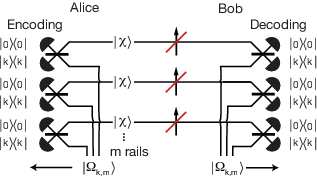
We now consider our protocol in detail. The protocol is shown in fig. 1. Consider two neighbouring nodes in a network, Alice and Bob, separated by a repeaterless link. Round one of our iterative protocol is identical to entanglement purification of Gaussian CV quantum states from Ref. Duan et al. 2000, however, our protocol includes an iterative procedure. Alice prepares copies of a pure two-mode squeezed vacuum (TMSV) state, in the Fock photon-number basis, with squeezing parameter . The unique entanglement measure, , for a bipartite pure state, , is given by the von Neumann entropy, , of the reduced state, i.e., , where . This means Alice initially prepares ebits of entanglement, where , where , , , and .
Alice shares the second mode of each of the pairs with Bob across the link. The error channel we consider is bosonic pure loss, modelled by mixing the data rails with vacuum modes of the environment, or a potential eavesdropper (Eve), on a beamsplitter with transmissivity .

Alice encodes the quantum information into a quantum-error-detecting code so that Bob can detect errors on his side. To do this, she performs a QND measurement of total photon number on the modes and obtains outcome (where the subscript refers to the round one of iteration), and shares this information with Bob via classical communication. Alice’s measurement projects the system before the channel onto a maximally-entangled state Duan et al. 2000
| (1) | ||||
| (2) |
where can be viewed as orthogonal basis states which form a quantum-error-detecting code, each composed of photons. We discuss the code in detail later. The pure maximally-entangled state has entanglement ebits with dimension , and the probability of Alice’s measurement outcome, , is . The dimension, , is the total number of ways identical photons can be arranged among the distinct rails.
Bob then performs a QND measurement of total photon number across the rails on his side to detect loss errors. If Bob obtains the outcome photons, and knows that Alice sent photons, then both Alice and Bob know that photons were lost. Bob’s QND measurement, with success probability , heralds a renormalised mixed state shared between Alice and Bob which does not depend on loss for any outcome . That is, together Alice’s and Bob’s QND measurements remove all dependence on loss and has exchanged success probability for entanglement, while they learn that photons were lost to the environment. All outcomes besides zero at Alice and Bob herald useful entanglement. If , they must do further rounds of purification (iteration) since the output state is not pure. If , then the output state is strictly pure and purification is complete in a single round. For a simpler protocol, Alice and Bob may post select on outcomes without further iteration. We show later in the paper that this single-shot protocol still gives excellent rates.
Explicitly, the global output state heralded by outcomes and is
| (3) |
where refer to the -rail quantum systems owned by Alice, Bob, and the environment, respectively, as shown in fig. 1. The full derivation of this state is in Supplementary Note 2. The factor is outside the sum, thus, we have the remarkable result that the renormalised output state shared between Alice and Bob does not depend on . Therefore, the entanglement shared between Alice and Bob also has no dependence on , which has been exchanged for probabilities.
Additional rounds of purification can purify more entanglement after the initial round. One approach is for Alice and Bob to locally perform QND measurements as in round one but on rails, and obtain outcomes , where refers to the round number. At round , there is no entanglement shared between Alice and Bob on the last rails and the photon number of each of these rails is completely known. At round , these last rails can be discarded while the rails should be kept.
Exact rate of iterative entanglement purification for finite numbers of rails. The rate of our purification protocol (in ebits per use) is maximised if Alice performs her first measurement offline (i.e., setting ) where she obtains outcome . For finite , there is a finite which optimises the rate. However, for large squeezing outcomes are dominated by with unity probability. Therefore, the large squeezing limit without pre-selection, is equivalent to with offline pre-selection.
Taking Alice’s first measurement to be done with result offline (which can be chosen in advance to optimise the rate or, for example, the practicality of the protocol), the rate for finite is
| (4) |
where the sum is constrained by
| (5) | ||||
| (6) | ||||
| (7) | ||||
| (8) | ||||
| (9) |
where the probability of success for a particular combination of outcomes, , for a given and is
| (10) |
where a maximally-entangled state is generated with entanglement
| (11) |
The rate for finite can be optimised over Alice’s initial outcome prepared offline and the number of rails as a function of . We numerically compute the rate in Supplementary Note 3 for small and . We show next that the highest rate of our iterative protocol achieves the capacity, , for and (i.e., ). We show this without having to compute eq. 4 directly which would be arduous.
Optimality of our protocol. The RCI Pirandola et al. 2009; García-Patrón et al. 2009, , gives an achievable lower bound on the distillable entanglement, , and on the optimal secret key rate. The RCI is defined in the Methods section. We will show that our protocol is optimal for entanglement distillation as and and that no entanglement is lost between rounds. We use the RCI as a benchmark to test the quality of our distillation procedure. The optimal distillation protocol implicit by the RCI is not required here since our scheme gives the same performance as the implicit optimal protocol round after round for large .
We require that the weighted average von Neumann entropy of the reduced pure states heralded after round one, , plus the average RCI of the failure states heralded after round one, , equals the RCI of the state before round one. Note that the RCI equals the von Neumann entropy for pure states. We have
| (12) |
in units of ebits per channel use, where
| (13) | ||||
| (14) |
where , where and . When the first round succeeds, the entanglement of the renormalised maximally-entangled pure-state shared between Alice and Bob heralded by outcomes is given by the von Neumann entropy of the reduced state:
| (15) |
which does not depend on the transmissivity, , nor the amount of two-mode squeezing, . When the first round fails, the RCI of the renormalised mixed state shared between Alice and Bob heralded by each pair of outcomes and is
| (16) |
which also does not depend on the transmissivity, , nor the amount of two-mode squeezing, . See Supplementary Note 2 for the derivation.
The amount of squeezing is scaled to infinity , such that Alice initially measures a large amount of photons and . Furthermore, from the fact that is a binomial distribution, Bob will most likely measure photons. Using these conditions, we show in Supplementary Note 3 that eq. 12 approaches
| (17) |
which ensures that round one of purification is optimal since there is no loss of rate after round one as , given that the average RCI at the end of the round equals the initial RCI of the protocol. Thus, there exists an optimal protocol to follow round one which can saturate the two-way assisted quantum capacity (the PLOB bound) using our protocol as an initial step. The entanglement is optimally exchanged for success probability.
Similarly, we prove in Supplementary Note 3 that round is optimal since there is no loss of rate at round as , up to the same factor, . This factor comes from Alice’s and Bob’s measurement of photon number.
To quantify this loss of entanglement, consider the protocol before the channel. We’ll see that for finite some entanglement is immediately lost after Alice’s QND measurement. Ref. Duan et al. 2000 defined the entanglement ratio, denoted by , as the average entanglement heralded by Alice’s QND measurement divided by the total initial entanglement , that is,
| (18) |
In the limit of a large number of rails for all , which means asymptotically Alice’s QND measurement heralds no loss of entanglement. However, for finite in the limit of large squeezing, . So, for finite number of rails some entanglement is lost since . This means we must take to get the highest rates.
Similarly, to quantify the entanglement lost at round , we define the entanglement ratio, , as the weighted average entanglement heralded at round over all outcomes normalised by the weighted entanglement heralded by outcome at the previous round, , that is,
| (19) |
where and . () and () are defined in eqs. 10 and 11, for a given (), and of course we can take for all since here we consider no loss channel. Many of the factors cancel giving the simple expression in eq. 19. Curiously, for large numbers of rails the amount of entanglement lost at round is the same as for round one, i.e., for all . This result ensures that “encoding” into photons is asymptotically optimal throughout the entire duration of our iterative procedure up to the factor , which approaches unity for large .
Achieving the capacity. The average rate in case of success of pure entanglement distilled at round in ebits per use of the channel is
| (20) |
and the average rate in case of failure of entanglement distilled at round in ebits per use of the channel is lower bounded by the average RCI
| (21) |
where is the probability from eq. 10 and is the RCI of the heralded states. Note is the Kronecker delta function. For the rate in case of success, the RCI equals the von Neumann entropy since the states are pure, . The entanglement in case of failure at round will be purified at a later round.
Since our protocol is optimal at round for and , we have the following expressions:
| (22) | ||||
| (23) |
for . We solve this system of equations by addition, and we find that the average rate in case of success of purification using our iterative procedure for and is
| (24) | ||||
| (25) | ||||
| (26) |
We achieve the capacity (PLOB) in the limit of a large number of rails, where and . See Supplementary Note 3 for the proof.
Achievable rates of repeater networks.
Our protocol purifies completely at the PLOB rate. Assuming ideal quantum memories are available, after teleportation (entanglement swapping) we achieve the the ultimate end-to-end rates of quantum communication networks by adopting the routing methods of Ref. Pirandola 2019. That is, the results can be extended beyond chains to consider more complex topologies and routing protocols Pirandola 2019. We describe details about entanglement swapping in Supplementary Note 4. We plot the highest rates of iterative purification as a function of total distance with no repeater and one repeater in fig. 2a (black lines) which coincide with the capacities. We also plot rates in fig. 2a for single-shot purification for finite where Alice and Bob stop after the first round which is a much more practical design. We discuss in detail those single-shot rates next.

Single-shot purification. Purification is complete after a single round if no photons are lost and Alice and Bob detect the same number of photons, . If Bob detects less photons than Alice, , further purification is required, however, it is most practical to disregard those outcomes and keep only the outcome which purifies in one shot. Alice’s measurement can be preselected and prepared offline, thus, improving the rate of a particular pair of outcomes. The single-shot rate for a given and can be quite close to the PLOB rate.
Recall that the optimal protocol implicit by the RCI is based on one-way classical communication García-Patrón et al. 2009, whereas, our iterative procedure requires two-way classical communication. Here, the single-shot protocol requires only one-way classical communication, like the implicit optimal protocol. Alice and Bob agree on the quantum-error-detecting code ( and ) in advance, so Alice does not need to send any classical information towards Bob. Bob only needs to send classical information towards Alice, telling her when the protocol succeeds. This greatly simplifies the required back-and-forth signalling in a quantum network.
Highest achievable rate for single-shot purification against the bosonic pure-loss channel. The rate of single-shot purification is as follows. The probability that Alice obtains outcome is , however, for the single-shot protocol we can incorporate this step into Alice’s state preparation and assume this is done offline such that . This means the rate will not depend on . When Bob obtains the outcome which matches Alice’s, , his probability is and the output state is pure with entanglement . Thus, the achievable rate of single-shot entanglement purification in ebits per use of the channel is
| (27) |
The rate is divided by the number of rails, , to compare directly with the PLOB bound Pirandola et al. 2017. This is required because Alice and Bob exploit a quantum channel whose single use involves the simultaneous transmission of distinct systems in a generally entangled state.
This rate is for a perfect implementation without any additional losses, errors, or noise. The protocol heralds pure states in a single attempt, so if we have ideal quantum memories, after entanglement swapping (see Supplementary Note 4 for details on entanglement swapping) we can distribute entanglement between ends of a network without any loss of rate, i.e., at the rate given by eq. 27 where is the transmissivity of the most destructive link.
Our optimised rate over and is shown in fig. 2a, without and with one quantum repeater (with a repeater, we assume ideal quantum memories). The PLOB bound can ultimately be broken at 46.3 km using single-shot purification between nodes and a single repeater for entanglement swapping. In fig. 2b, we show the ratio of our optimised single-shot rate with the PLOB bound, showing that at long distances the protocol falls short of the PLOB bound by just a factor of , and remarkably, our rate approaches at short distances. At short distances, the rate is optimised for larger while at long distances is always optimal since the probability that photons arrive scales like at long distances. The optimal number of rails is about at most distances (including long distances) since increasing the number of rails decreases the rate like . Larger is sometimes optimal at short distances.
The rate of our single-shot purification protocol is unable to saturate the ultimate limit because we postselect on Bob’s outcomes, throwing away useful entanglement when and . Keeping all measurement outcomes, the rate increases, however, it is less practical to do so.
Quantum error detection. In this section, we describe our single-shot purification protocol as quantum error detection. Consider encoding an arbitrary finite-dimensional single-rail state with dimension :
| (28) |
where .
The code is a subspace with dimensions (-dimensional), a subspace of the infinite-dimensional Hilbert space chosen to detect loss errors nondeterminisitically. It is represented by the projector onto the subspace
| (29) |
where are the orthogonal basis states (code words) which make up the code subspace (code space), where is the logical label. Note is the number of photons in the th rail, which depends on the logical label , as well as and where . There are code words, i.e., for a given code the set of code words is . Quantum information up to dimension can faithfully be transmitted to Bob, conditioned that he detects no errors. Photon loss (and photon gains) will result in states outside of code space, which we can distinguish as an error.
The set of logical states forming the -dimensional basis of the code consists of all possible ways identical photons can be arranged among the distinct rails. For example, . The code space is a subspace of the full Hilbert space of the rails which introduces the redundancy required for error detection, that is, photons and rails can encode -dimensional states. The dimension grows rapidly with and . For example, with just photons and rails, we can efficiently encode 70-dimensional states, i.e., truncated at Fock number , with success probability . This is a great advantage over noiseless linear amplification, for example, if we choose the gain of the amplifier to be to overcome the loss then the success probability is , totally impractical. Furthermore, noiseless linear amplification fails to purify completely and cannot completely overcome the loss.
The encoding step is
| (30) |
which maps Fock states, , from a single mode to the code words, . The combined operation of encoding, loss, and decoding is a completely-positive trace-non-increasing map
| (31) |
where is the map for independent applications of the pure-loss channel on the rails, the decoding step, , performs a QND measurement of the total photon number, and if photons arrive, then it successfully decodes back to single rail. The decoding step succeeds only if no photons are lost. The combined operation, , is a scaled identity map up to the th Fock state, thus, the protocol succeeds with success probability with unit fidelity.
The input state may be entangled with another mode. For example, we may consider encoding one arm of an arbitrary entangled state, . In this case, the operation, , acts on Bob’s mode only and Alice leaves her mode alone. The final state shared between Alice and Bob is , where is the initial state and is the identity on mode . Note there is still useful entanglement if photons are lost. The entanglement-distribution rate of single-shot error detection for a maximally-entangled initial state is given by eq. 27, showing that error detection and purification indeed are equivalent.
One might consider using purification to distribute Gaussian entanglement for long-distance CV QKD between trusted end users of a network, performing the entanglement-based CV-QKD protocol based on homodyne detection J. Cerf et al. 2001; Gottesman and Preskill 2001 or heterodyne detection Weedbrook et al. 2004. Consider the initial data state to be a truncated TMSV state with dimension given by
| (32) |
The state is Gaussian except for the hard truncation in Fock space. The protocol works as follows. First, truncated TMSV states, , are distributed using our single-shot purification scheme between all repeater nodes and held in quantum memories. Once successful, CV entanglement swapping is used to entangle the end users who use the entanglement to perform CV QKD. While the purification scheme can be complex (depending on the chosen protocol size), the CV entanglement swapping is simple. It works by performing dual-homodyne measurements on some of the modes, followed by conditional displacements, swapping the entanglement Hoelscher-Obermaier and van Loock 2011, see Supplementary Note 4 for details on how to compute the secret key rate.
A simple example: the qubit code. The simplest nontrivial code uses a single photon, , in two rails, , (i.e., unary dual-rail) and protects qubit systems, , from loss. It is equivalent to the original purification protocol from Ref. Bennett et al. 1996, but in this context we use it to purify entanglement completely from pure loss to first order in Fock space and we can protect arbitrary single-rail qubit states from loss. The code words can be defined and . The projector onto the code space is . The encoding step is
| (33) | ||||
| (34) |
which maps the vacuum component of the data mode onto a single photon of the second rail and the single-photon component of the data mode onto a single photon of the first rail. If either of these photons is lost, the protocol fails. The success probability is . The maximum single-shot rate in ebits per use is , as shown by the dashed line in fig. 2a (with and without a repeater).
Physical implementation. Entanglement purification (iterative and single shot) requires joint QND measurements on multiple rails. These measurements can be performed via controlled-SUM quantum gates and photon number-resolving measurements (see Supplementary Note 5, for example). Another technique is to use high finesse cavities and cross–Kerr nonlinearities Duan et al. 2000.
More simply, our scheme can be implemented using beamsplitters and photon-number-resolving detectors, however, it also requires an entangled resource state, . This is a common technique in linear optics Yan et al. 2021a; Yan et al. 2021b. See Ref. Kok et al. 2007 for a review of quantum information processing using linear optics. The resource state can also be generated using linear optics and photon-number measurements. That is, we have a simple method of implementing our protocol, though at some cost to the success probability.
We focus on the single-shot linear-optics protocol, shown in fig. 3. Alice shares entangled states, , with Bob. Note each rail could have a different , distilling different amounts of entanglement between Alice and Bob at the end of the protocol, however, maximal entanglement is heralded when all rails have the same value of . Alice and Bob each prepare locally multimode resource states, , consisting of modes. We assume they do this offline so it does not affect the quantum communication rate:
| (35) |
where are Fock states, are “anticorrelated” code words. Writing the usual code words in the Fock basis as , where is the number of photons in the th rail, and where , recalling that the code space was defined as the set of all states with this property, then . The coefficients, , are
| (36) |
The last modes of are fed into the beamsplitters with the distributed entanglement and are measured by photon-number detectors. The first mode is kept locally by the user and remains at the end of the protocol, as shown in fig. 3.
Detecting photons means there were no loss events since . That is, all photons are accounted for in the circuit and the output state is strictly pure. There may be useful entanglement for measurement outcomes other than at each pair of detectors, and further purification (iteration) can increase the rate, but we do not consider it due to practicality.
Adjusting the amount of entanglement prepared for each rail, adjusting the loss on each rail, or selecting different coefficients in the resource state, , results in a different output state, which may be useful for certain tasks. For example, if the entangled states prepared for each rail are identical and have the same amount of squeezing and is chosen as in eq. 36, then a maximally-entangled state will be heralded between Alice and Bob at the output. For another example, consider the dual-rail case (), if the second rail is maximally entangled and is chosen as in eq. 36, then the output state is the initial state of the top rail. This tuning of the circuit parameters is useful, for instance, for CV QKD where the target state is a truncated TMSV state.
The linear-optics scheme detects all errors and outputs a pure state. There is, however, an additional success probability penalty using linear optics because of Bob’s decoding measurement. We assume Alice prepares offline, then the success probability is
| (37) |
which depends on . Compare this with the ideal purification protocol where which does not depend on . The penalty paid for using linear optics is mainly due to the exponential factor, which is painful for anything other than , where . For more details we refer you to Supplementary Note 6.
The linear-optics circuit leads naturally to a controlled-SUM gate using linear optics and number measurements, albeit with distorted coefficients (this distortion ultimately has no effect in our protocol since we immediately measure the state). For the interested reader, we refer you to Supplementary Note 5 for more details.
Since Alice’s encoded state is prepared offline, it is useful to consider more generally that she encodes an arbitrary state into the code: .
Preparation of resource states. For our linear-optics and number measurement circuit, the resource state, , and Alice’s encoded state she prepares offline, are multi-mode entangled states. Once these states are prepared, our scheme requires just beamsplitters and photon detectors. One practical way to prepare these states is to use a Gaussian Boson Sampler (GBS) Hamilton et al. 2017 and postselecting on a specific photon-number-resolving measurement click pattern on some of the modes of the output Su et al. 2019; Quesada et al. 2019. This allows our scheme to be implemented entirely using linear-optics and number measurements. Using the GBS method for the simplest scheme with and , we have found the resource state, , can be prepared with high fidelity, , with success probability . This was found by optimising the parameters of a GBS network via a machine learning algorithm called “basin hopping” Sabapathy et al. 2019. In Jos, we have provided our code which implements this algorithm, as well as the parameter set we found that generates this resource state. Alternatively, adaptive phase measurements Ralph et al. 2005 can be used to prepare the needed resource states directly from dual-rail Bell pairs or GHZ-like states which may have a higher probability of success.
Experimental imperfections. Our linear-optics circuit is robust to loss. The quality of the state Alice sends can be managed since her encoding is done offline. In any case, we are interested in the noise introduced by the protocol, not the noise in the initial state we are trying to transmit. The measurement and detection scheme at Bob’s side is such that all photons are accounted for, so if Alice’s encoding is perfect, the protocol can correctly identify if any photons are lost in the channel or at the detectors. More details are presented in Supplementary Note 6, where we also perform a numerical simulation incorporating inefficient detectors with dark counts, and a thermal-noise channel. Our protocol is robust to practical values of these imperfections.
The directionality issue. Often in quantum communications it is best if quantum states propagate in one preferred direction (from Alice towards Bob) when reverse reconciliation is used. This is a persistent problem in CV quantum communications. For instance, CV measurement-device-independent protocols Ma et al. 2014; Zhang et al. 2014; Ottaviani et al. 2015; Pirandola et al. 2015 work only in an extremely asymmetric configuration, with the node (ineffective as a repeater) positioned close to one of the trusted parties. This directionality problem is also present in the repeater protocols considered in Ref Dias et al. 2020; Ghalaii and Pirandola 2020, where they work best in one direction, which for reverse reconciliation is again from Alice towards Bob. Our purification schemes allow states to propagate in any direction in a quantum network since the output states are pure. Using purification for CV-QKD works the same for both direct and reverse reconciliations. We have no directionality problem. This is an important requirement for large CV networks. Note that the memoryless CV repeater protocol introduced in Ref. Winnel et al. 2021 also fixes the directionality problem.
Discussion
We have presented a physical protocol which achieves the two-way assisted quantum capacity of the pure-loss channel Pirandola et al. 2017. Error correction requires short distances between neighbouring repeater nodes, while in contrast, we showed simple error detection can saturate the PLOB bound. An open question is what protocol can saturate the fundamental limits for added thermal noise and close the gap between the theoretical upper and lower bounds Pirandola et al. 2017. Furthermore, can error detection saturate the ultimate limits for other noise models, for instance, dephasing?
Our protocol is an optimal one and can be performed using CSUM quantum gates and measurements. However, it is unknown whether other gates and measurements may also achieve the capacity, and if they can do so more efficiently, i.e., approaching the PLOB bound more quickly with the number of iteration rounds, .
Our ultimate protocol is experimentally challenging since it requires iterative purification steps. However, we show that by simplifying our protocol to just a single round of purification, we can still achieve excellent rates. This is superior to other nondeterministic techniques such as noiseless linear amplification where it is impossible to remove all effects of loss.
Our purification protocol can be implemented using linear-optics and number measurements. This does introduce some probability penalty (which does not depend on the loss), however, having an all-optical design is experimentally convenient.
One limitation of our results is the requirement for high-performance quantum memories. However, purification outputs pure states which is extremely beneficial. Firstly, pure states can handle a higher amount of decoherence coming from nonideal quantum memories. Secondly, distributing pure states will prevent how much thermal noise builds up across a network during entanglement swapping. Finally, purity may be beneficial for both point-to-point and repeater-assisted CV QKD, improving the signal-to-noise ratio and decreasing Eve’s knowledge of the key, speeding up the classical post-processing part of the protocol.
Thus, purification is inherently a useful technique for overcoming the unavoidable losses in quantum communication networks. Remarkably, purification can be employed totally using linear optics and number measurements and is compatible with existing DV and CV infrastructure. Finally, we remark that since the lossy entanglement is completely purified, it can be used for exotic tasks, such as device-independent quantum key distribution and demonstrating Bell nonlocalities, over much longer distances than previously imagined.
Methods
Noise model. Bosonic pure loss is the dominant source of noise for many quantum communication tasks. The pure-loss channel is equivalent to introducing a vacuum mode and mixing the data state on a beamsplitter with transmissivity . The Kraus-operator representation of the single-mode pure-loss channel is Chuang et al. 1997
| (38) |
with Kraus operators associated with losing photons to the environment, where and are the single-mode annihilation and creation operators, respectively, and is the photon-number operator.
Reverse coherent information. Take a maximally entangled state of two systems and . Propagating the system through the quantum channel defines the Choi state of the channel. Then the reverse coherent information represents a lower bound for the distillable entanglement and for the optimal secret key rate. The reverse coherent information of a state is defined as García-Patrón et al. 2009
| (39) |
where and are von Neumann entropies of and respectively. The von Neumann entropy of is .
Acknowledgements.
We thank Ozlem Erkilic, Sebastian Kish, Ping Koy Lam, Syed Assad, Deepesh Singh, and Josephine Dias for valuable discussions during this investigation. We thank Deepesh Singh for an alternative proof given in Supplementary Note 7. This research was supported by the Australian Research Council (ARC) under the Centre of Excellence for Quantum Computation and Communication Technology (CE170100012).Author contributions
All authors contributed to this work extensively and to the writing of the manuscript.
Competing Interests statement
All authors reported no potential competing interests.
Data availability statement
The datasets generated during and analysed during the current study are available from the corresponding author on reasonable request.
References
- Gisin and Thew (2007) N. Gisin and R. Thew, “Quantum communication,” Nature Photonics 1, 165–171 (2007).
- Cerf et al. (2007) N. Cerf, G. Leuchs, and E. Polzik, Quantum Information With Continuous Variables of Atoms and Light (2007).
- Proctor et al. (2018) T. J. Proctor, P. A. Knott, and J. A. Dunningham, “Multiparameter estimation in networked quantum sensors,” Phys. Rev. Lett. 120, 080501 (2018).
- Ge et al. (2018) W. Ge, K. Jacobs, Z. Eldredge, A. V. Gorshkov, and M. Foss-Feig, “Distributed quantum metrology with linear networks and separable inputs,” Phys. Rev. Lett. 121, 043604 (2018).
- Zhuang et al. (2018) Q. Zhuang, Z. Zhang, and J. H. Shapiro, “Distributed quantum sensing using continuous-variable multipartite entanglement,” Phys. Rev. A 97, 032329 (2018).
- Van Meter and Devitt (2016) R. Van Meter and S. J. Devitt, “The path to scalable distributed quantum computing,” Computer 49, 31 (2016).
- Danos et al. (2007) V. Danos, E. D’Hondt, E. Kashefi, and P. Panangaden, “Distributed measurement-based quantum computation,” Electronic Notes in Theoretical Computer Science 170, 73 (2007), proceedings of the 3rd International Workshop on Quantum Programming Languages (QPL 2005).
- Pirandola et al. (2020) S. Pirandola, U. L. Andersen, L. Banchi, M. Berta, D. Bunandar, R. Colbeck, D. Englund, T. Gehring, C. Lupo, C. Ottaviani, and et al., “Advances in quantum cryptography,” Advances in Optics and Photonics 12, 1012 (2020).
- Xu et al. (2020) F. Xu, X. Ma, Q. Zhang, H.-K. Lo, and J.-W. Pan, “Secure quantum key distribution with realistic devices,” Reviews of Modern Physics 92 (2020), 10.1103/revmodphys.92.025002.
- Pirandola et al. (2009) S. Pirandola, R. García-Patrón, S. L. Braunstein, and S. Lloyd, “Direct and reverse secret-key capacities of a quantum channel,” Phys. Rev. Lett. 102, 050503 (2009).
- Takeoka et al. (2014) M. Takeoka, S. Guha, and M. M. Wilde, “Fundamental rate-loss tradeoff for optical quantum key distribution,” Nature Communications 5 (2014), 10.1038/ncomms6235.
- Kimble (2008) H. J. Kimble, “The quantum internet,” Nature 453, 1023–1030 (2008).
- García-Patrón et al. (2009) R. García-Patrón, S. Pirandola, S. Lloyd, and J. H. Shapiro, “Reverse coherent information,” Phys. Rev. Lett. 102, 210501 (2009).
- Pirandola et al. (2017) S. Pirandola, R. Laurenza, C. Ottaviani, and L. Banchi, “Fundamental limits of repeaterless quantum communications,” Nature Communications 8 (2017), 10.1038/ncomms15043.
- Pirandola (2019) S. Pirandola, “End-to-end capacities of a quantum communication network,” Communications Physics 2 (2019), 10.1038/s42005-019-0147-3.
- Munro et al. (2015) W. J. Munro, K. Azuma, K. Tamaki, and K. Nemoto, “Inside quantum repeaters,” IEEE Journal of Selected Topics in Quantum Electronics 21, 78 (2015).
- Muralidharan et al. (2016) S. Muralidharan, L. Li, J. Kim, N. Lütkenhaus, M. D. Lukin, and L. Jiang, “Optimal architectures for long distance quantum communication,” Scientific Reports 6, 20463 (2016).
- Giedke and Ignacio Cirac (2002) G. Giedke and J. Ignacio Cirac, “Characterization of gaussian operations and distillation of gaussian states,” Phys. Rev. A 66, 032316 (2002).
- Eisert et al. (2002) J. Eisert, S. Scheel, and M. B. Plenio, “Distilling gaussian states with gaussian operations is impossible,” Phys. Rev. Lett. 89, 137903 (2002).
- Namiki et al. (2014) R. Namiki, O. Gittsovich, S. Guha, and N. Lütkenhaus, “Gaussian-only regenerative stations cannot act as quantum repeaters,” Phys. Rev. A 90, 062316 (2014).
- Nielsen and Chuang (2011) M. A. Nielsen and I. L. Chuang, Quantum Computation and Quantum Information: 10th Anniversary Edition, 10th ed. (Cambridge University Press, USA, 2011).
- Braunstein and van Loock (2005) S. L. Braunstein and P. van Loock, “Quantum information with continuous variables,” Reviews of Modern Physics 77, 513–577 (2005).
- Yonezawa and Furusawa (2008) H. Yonezawa and A. Furusawa, “Continuous-variable quantum information processing with squeezed states of light,” (2008), arXiv:0811.1092 [quant-ph] .
- Weedbrook et al. (2012) C. Weedbrook, S. Pirandola, R. García-Patrón, N. J. Cerf, T. C. Ralph, J. H. Shapiro, and S. Lloyd, “Gaussian quantum information,” Reviews of Modern Physics 84, 621–669 (2012).
- Serafini (2017) A. Serafini, Quantum Continuous Variables: A Primer of Theoretical Methods (CRC Press, 2017).
- Kumar et al. (2015) R. Kumar, H. Qin, and R. Alléaume, “Coexistence of continuous variable QKD with intense DWDM classical channels,” New Journal of Physics 17, 043027 (2015).
- Dias and Ralph (2017) J. Dias and T. C. Ralph, “Quantum repeaters using continuous-variable teleportation,” Physical Review A 95 (2017), 10.1103/physreva.95.022312.
- Furrer and Munro (2018) F. Furrer and W. J. Munro, “Repeaters for continuous-variable quantum communication,” Physical Review A 98 (2018), 10.1103/physreva.98.032335.
- Seshadreesan et al. (2020) K. P. Seshadreesan, H. Krovi, and S. Guha, “Continuous-variable quantum repeater based on quantum scissors and mode multiplexing,” Phys. Rev. Research 2, 013310 (2020).
- Ghalaii and Pirandola (2020) M. Ghalaii and S. Pirandola, “Capacity-approaching quantum repeaters for quantum communications,” Physical Review A 102 (2020), 10.1103/physreva.102.062412.
- Dias et al. (2020) J. Dias, M. S. Winnel, N. Hosseinidehaj, and T. C. Ralph, “Quantum repeater for continuous-variable entanglement distribution,” Physical Review A 102 (2020), 10.1103/physreva.102.052425.
- Winnel et al. (2021) M. S. Winnel, J. J. Guanzon, N. Hosseinidehaj, and T. C. Ralph, “Overcoming the repeaterless bound in continuous-variable quantum communication without quantum memories,” (2021), arXiv:2105.03586 [quant-ph] .
- Ralph and Lund (2009) T. C. Ralph and A. P. Lund, “Nondeterministic noiseless linear amplification of quantum systems,” AIP Conference Proceedings 1110, 155 (2009), https://aip.scitation.org/doi/pdf/10.1063/1.3131295 .
- Winnel et al. (2020) M. S. Winnel, N. Hosseinidehaj, and T. C. Ralph, “Generalized quantum scissors for noiseless linear amplification,” Phys. Rev. A 102, 063715 (2020).
- Guanzon et al. (2021) J. J. Guanzon, M. S. Winnel, A. P. Lund, and T. C. Ralph, “Ideal quantum tele-amplification up to a selected energy cut-off using linear optics,” (2021), arXiv:2110.03172 [quant-ph] .
- Fiurášek (2021) J. Fiurášek, “Teleportation-based noiseless quantum amplification of coherent states of light,” (2021), arXiv:2110.06040 [quant-ph] .
- Blandino et al. (2012) R. Blandino, A. Leverrier, M. Barbieri, J. Etesse, P. Grangier, and R. Tualle-Brouri, “Improving the maximum transmission distance of continuous-variable quantum key distribution using a noiseless amplifier,” Phys. Rev. A 86, 012327 (2012).
- McMahon et al. (2014) N. A. McMahon, A. P. Lund, and T. C. Ralph, “Optimal architecture for a nondeterministic noiseless linear amplifier,” Phys. Rev. A 89, 023846 (2014).
- Blandino et al. (2015) R. Blandino, M. Barbieri, P. Grangier, and R. Tualle-Brouri, “Heralded noiseless linear amplification and quantum channels,” Phys. Rev. A 91, 062305 (2015).
- Pandey et al. (2013) S. Pandey, Z. Jiang, J. Combes, and C. M. Caves, “Quantum limits on probabilistic amplifiers,” Physical Review A 88 (2013), 10.1103/physreva.88.033852.
- Fowler et al. (2010) A. G. Fowler, D. S. Wang, C. D. Hill, T. D. Ladd, R. Van Meter, and L. C. L. Hollenberg, “Surface code quantum communication,” Physical Review Letters 104 (2010), 10.1103/physrevlett.104.180503.
- Gottesman (2009) D. Gottesman, “An introduction to quantum error correction and fault-tolerant quantum computation,” (2009), arXiv:0904.2557 [quant-ph] .
- Gottesman et al. (2001) D. Gottesman, A. Kitaev, and J. Preskill, “Encoding a qubit in an oscillator,” Physical Review A 64 (2001), 10.1103/physreva.64.012310.
- Noh et al. (2019) K. Noh, V. V. Albert, and L. Jiang, “Quantum capacity bounds of gaussian thermal loss channels and achievable rates with gottesman-kitaev-preskill codes,” IEEE Transactions on Information Theory 65, 2563–2582 (2019).
- Bennett et al. (1996) C. H. Bennett, G. Brassard, S. Popescu, B. Schumacher, J. A. Smolin, and W. K. Wootters, “Purification of noisy entanglement and faithful teleportation via noisy channels,” Physical Review Letters 76, 722–725 (1996).
- Duan et al. (2000) L.-M. Duan, G. Giedke, J. I. Cirac, and P. Zoller, “Entanglement purification of gaussian continuous variable quantum states,” Phys. Rev. Lett. 84, 4002 (2000).
- Horodecki et al. (2005) K. Horodecki, M. Horodecki, P. Horodecki, and J. Oppenheim, “Secure key from bound entanglement,” Physical Review Letters 94 (2005), 10.1103/physrevlett.94.160502.
- J. Cerf et al. (2001) N. J. Cerf, M. Lévy, and G. Van Assche, “Quantum distribution of gaussian keys using squeezed states,” Phys. Rev. A 63, 052311 (2001).
- Gottesman and Preskill (2001) D. Gottesman and J. Preskill, “Secure quantum key distribution using squeezed states,” Physical Review A 63 (2001), 10.1103/physreva.63.022309.
- Weedbrook et al. (2004) C. Weedbrook, A. M. Lance, W. P. Bowen, T. Symul, T. C. Ralph, and P. K. Lam, “Quantum cryptography without switching,” Phys. Rev. Lett. 93, 170504 (2004).
- Hoelscher-Obermaier and van Loock (2011) J. Hoelscher-Obermaier and P. van Loock, “Optimal gaussian entanglement swapping,” Phys. Rev. A 83, 012319 (2011).
- Yan et al. (2021a) P.-S. Yan, L. Zhou, W. Zhong, and Y.-B. Sheng, “Feasible measurement-based entanglement purification in linear optics,” Opt. Express 29, 9363 (2021a).
- Yan et al. (2021b) P.-S. Yan, L. Zhou, W. Zhong, and Y.-B. Sheng, “Measurement-based entanglement purification for entangled coherent states,” Frontiers of Physics 17, 21501 (2021b).
- Kok et al. (2007) P. Kok, W. J. Munro, K. Nemoto, T. C. Ralph, J. P. Dowling, and G. J. Milburn, “Linear optical quantum computing with photonic qubits,” Reviews of Modern Physics 79, 135–174 (2007).
- Hamilton et al. (2017) C. S. Hamilton, R. Kruse, L. Sansoni, S. Barkhofen, C. Silberhorn, and I. Jex, “Gaussian boson sampling,” Phys. Rev. Lett. 119, 170501 (2017).
- Su et al. (2019) D. Su, C. R. Myers, and K. K. Sabapathy, “Conversion of gaussian states to non-gaussian states using photon-number-resolving detectors,” Phys. Rev. A 100, 052301 (2019).
- Quesada et al. (2019) N. Quesada, L. G. Helt, J. Izaac, J. M. Arrazola, R. Shahrokhshahi, C. R. Myers, and K. K. Sabapathy, “Simulating realistic non-gaussian state preparation,” Phys. Rev. A 100, 022341 (2019).
- Sabapathy et al. (2019) K. K. Sabapathy, H. Qi, J. Izaac, and C. Weedbrook, “Production of photonic universal quantum gates enhanced by machine learning,” Phys. Rev. A 100, 012326 (2019).
- (59) https://github.com/JGuanzon/state-finder.
- Ralph et al. (2005) T. C. Ralph, A. P. Lund, and H. M. Wiseman, “Adaptive phase measurements in linear optical quantum computation,” Journal of Optics B: Quantum and Semiclassical Optics 7, S245–S249 (2005).
- Ma et al. (2014) X.-C. Ma, S.-H. Sun, M.-S. Jiang, M. Gui, and L.-M. Liang, “Gaussian-modulated coherent-state measurement-device-independent quantum key distribution,” Physical Review A 89 (2014), 10.1103/physreva.89.042335.
- Zhang et al. (2014) Y.-C. Zhang, Z. Li, S. Yu, W. Gu, X. Peng, and H. Guo, “Continuous-variable measurement-device-independent quantum key distribution using squeezed states,” Physical Review A 90 (2014), 10.1103/physreva.90.052325.
- Ottaviani et al. (2015) C. Ottaviani, G. Spedalieri, S. L. Braunstein, and S. Pirandola, “Continuous-variable quantum cryptography with an untrusted relay: Detailed security analysis of the symmetric configuration,” Physical Review A 91 (2015), 10.1103/physreva.91.022320.
- Pirandola et al. (2015) S. Pirandola, C. Ottaviani, G. Spedalieri, C. Weedbrook, S. L. Braunstein, S. Lloyd, T. Gehring, C. S. Jacobsen, and U. L. Andersen, “High-rate measurement-device-independent quantum cryptography,” Nature Photonics 9, 397 (2015).
- Chuang et al. (1997) I. L. Chuang, D. W. Leung, and Y. Yamamoto, “Bosonic quantum codes for amplitude damping,” Phys. Rev. A 56, 1114 (1997).
Supplementary Notes
Supplementary Note 1 Noiseless linear amplification and entanglement swapping cannot completely purify entanglement
Noiseless linear amplification is a distinguished technique for the distillation of continuous-variable (CV) entanglement but it is unable to purify completely from loss. It is unable to return a loss-attenuated entangled state back to its original loss-free entangled state.
To see this, consider pure loss acting on one mode of a CV two-mode squeezed vacuum (TMSV) state with the squeezing parameter . Pure loss is equivalent to interacting the data mode with vacuum on a beamsplitter with transmissivity . Consider ideal noiseless linear amplification Pandey et al. 2013 with gain applied to the lossy arm to correct the loss. The final state after ideal noiseless linear amplification of the lossy mode results in another lossy mixed TMSV state but with different parameters:
| (S1) |
where is the completely-positive trace-preserving (CPTP) map for the pure-loss channel with transmissivity . The new parameters, and , are related to the old parameters, and , in the following way: Blandino et al. 2012; McMahon et al. 2014; Blandino et al. 2015
| (S2) | ||||
| (S3) |
The effective loss is zero when which for finite gain is only possible when . This means that it is impossible to completely correct loss using noiseless linear amplification. Also, as , the success probability tends to zero.
Entanglement swapping is another technique that can distil entanglement, however, it can be thought of as noiseless linear amplification with some loss distributed across the measurement Winnel et al. 2021; Guanzon et al. 2021, thus, entanglement swapping is also unable to completely purify CV entanglement. Other distillation techniques such as photon subtraction are also strictly limited in their purification abilities Zhang and van Loock 2010.
Noiseless linear amplification is nondeterministic. Ideal noiseless linear amplification is unphysical since the success probability is zero. Physical noiseless linear amplification is possible with a non-zero success probability by considering an energy cutoff. For instance, consider noiseless linear amplification which amplifies and truncates the input state at Fock number (where is the dimension of the output state), then the success probability scales like . Our purification scheme uses the entanglement between multiple modes so larger states can be protected against loss with a much higher success probability than noiseless linear amplification. Our success probability depends on the number of photons in the code, not the dimension of the state that is encoded. Our single-shot purification scheme has the improved success probability where in general . Furthermore, purification removes completely the effect of pure loss since errors are detected, while noiseless linear amplification is unable to do this.
To summarise, noiseless linear amplification and entanglement swapping (i.e., techniques for the first and second generations of quantum repeaters) fail to saturate the ultimate rate limits under pure loss for two reasons: 1. the output entangled states are strictly non-pure for any amount of loss and for finite gain, and 2. the success probability depends on the energy cutoff and tends to zero for large input states. Whereas, our purification scheme purifies completely and has a success probability that scales optimally with loss in the sense that the highest average rate of entanglement purification saturates the capacity (the PLOB bound Pirandola et al. 2017).
Supplementary Note 2 Derivation of purified states generated between Alice and Bob
In this Supplementary Note, we derive the purified states heralded by Alice’s and Bob’s QND measurements.
Heralded states after round one of purification
In this section, we derive the heralded states (equation (3) of the main text) during round one.
Alice prepares copies of infinite-dimensional TMSV states, , where is the squeezing parameter. Then, she performs a mode-blind QND measurement on her side, and obtains an outcome of total photons. This measurement projects the TMSV states onto a maximally-entangled state, , with dimension , entanglement , and success probability . After Alice obtains outcome , Alice has the following maximally-entangled state:
| (S4) |
where refers to the quantum system Alice keeps and refers to the quantum system which will be sent to Bob.
Alice propagates Bob’s modes () across independent pure-loss channels. The pure loss is equivalent to introducing vacuum modes and mixing those with the data rails on beamsplitters of transmissivity . We label the beamsplitter transformations which interact modes and . The state after this interaction is
| (S5) | ||||
where is the number of photons lost from mode to .
Finally, Bob performs a QND measurement and obtains an outcome of total photons. The terms that survive in eq. S5 are those components where Bob’s modes have total photons which add up to , that is, . The total number of lost photons is the difference between Alice and Bob’s outcomes, . Thus, the unnormalised final state shared between Alice and Bob is
| (S6) |
which is equation (3) of the main text as required.
We can calculate the success probability (i.e., the probability to successfully get this output state) as follows
| (S7) | ||||
| (S8) | ||||
| (S9) | ||||
| (S10) | ||||
| (S11) |
We used the generalized Vandermonde identity to simplify the inner summation to ; this does not depend on the outer summation, which has terms. We can assign and , where we can interpret as a joint probability distribution. Remarkably, while this success probability depends on the transmissivity , the renormalised output state
| (S12) |
shared between Alice and Bob does not depends on .
Round two of purification
Recall that in the first round, Alice obtains outcome and Bob obtains outcome . They share the following state:
| (S13) |
Let us firstly consider the case when , then thus the output state is:
| (S14) |
We can see that the environment modes are all vacuum states and are separable from the state. When the state is purified in a single shot, and we do not need a second round.
Now, consider the case when , we will need further rounds of purification. In the second round, one option for further purification is to measure the total photon number on rails instead of all rails. This means they learn if some errors happened in the th rail, or in the first rails. If Alice obtains outcome and Bob obtains outcome , they share the state:
| (S15) |
If and , then no errors occurred in the first rails and the output state is , so the th rail is in a definite quantum state with no entanglement so this rail should be discarded. The rest of the modes are not entangled with the environment, so Alice and Bob’s state of these rails is pure.
Finally, if , we need still further purification rounds. After iterative rounds, we show next that we achieve the capacity as .
Supplementary Note 3 Optimality of our protocol and rates
In this Supplementary Note, we show that our protocol is optimal for entanglement distillation and achieves the two-way assisted capacity of the pure-loss channel (the PLOB bound) as and .
Proof that the first round is optimal
In this section, we show that the first round is optimal in the limit that and provide a lower bound on the distillable entanglement by directly calculating the average reverse coherent information (RCI).
The RCI gives a lower bound on the distillable entanglement and is given by (see Methods and Ref. García-Patrón et al. 2009)
| (S16) |
where and are the von Neumann entropies of and respectively, where .
For our iterative purification protocol, the average RCI per channel use is
| (S17) |
where is the probability of Alice and Bob obtaining outcomes and , heralding a state with RCI, . is the average entanglement of the pure states where the RCI is equal to the von Neumann entropy (when ):
| (S18) |
and is the average RCI of the failed terms (when ):
| (S19) |
The sum over terminates at since Bob cannot obtain outcomes . Notice the Kronecker delta in these equations highlights that the only difference between eq. S18 and eq. S19 is the constraint: for S18 and for S19. That way, it is easy to see that the total weighted average rate of success and failure is , without constraint.
We calculate the RCI, , of the normalised state shared between Alice and Bob conditioned on measurement outcomes at Alice and at Bob, where refers to the -mode system of the environment. The entropy of Alice’s system is , where the dimensionality is the number of ways photons can be arranged in modes, i.e., . Furthermore, since the global state is pure, we can use the self-duality property of the von Neumann entropy to calculate the entropy of Alice and Bob’s system
| (S20) |
That is, the environment holds the purification of Alice and Bob’s state. The entropy of the environment modes is , where is the number of ways photons can be arranged in modes, i.e., . This follows from the fact that the QND measurement is mode blind and we know for certain that photons were lost to the environment, but we do not know on which modes these losses occurred.
The output state , shown in equation (3) of the main text, shows that the arrangements of photons do not depend on or and are distributed with equal weights. We confirmed this directly by computing Eve’s information from the density matrix for the simplest cases.
Therefore, using eq. S16, the RCI for the renormalised state is
| (S21) |
This dimension ratio can be rewritten in a more useful form
| (S22) |
Alice is free to prepare her state offline. Hence, let us further simplify the rate expression by conditioning on Alice having already measured photons (i.e., fixed value),
| (S23) |
Note this rate does not depend on , since this conditional probability means only Bob’s measurement probability contributes to the rate .
For small , the most likely outcomes of Alice’s QND measurement is a small number of photons. As squeezing increases, Alice will more often detect a larger number of photons. We are interested in the large energy limit , since our aim is to saturate the PLOB bound. In this limit, the squeezed states become , hence Alice obtains large numbers of photons with unit probability. We have proven in section Supplementary Note 7 the following asymptotic relation
| (S24) |
Thus, our rate expression simplifies to
| (S25) | ||||
| (S26) |
At this point, we note that is a binomial distribution; this means that both the expected value and the most likely value Bob will measure is photons. From this physical intuition, we expect only terms near are important, hence the sum should simplify to . We can confirm this formally by firstly noting the binomial distribution moments are
| (S27) |
where we note only the term in the summation has the factor required to survive the limit. Note that are the Stirling numbers of the second kind (i.e., an integer independent of ), and resolves to for the relevant case. Thus, from the Taylor series expansion of the logarithm we have
| (S28) | ||||
| (S29) | ||||
| (S30) | ||||
| (S31) |
Finally, in the limit that , we have shown that the first step of our protocol is optimal since the average RCI equals the channel capacity of the pure-loss channel (the PLOB bound).
Optimality of our protocol at each round
In this section, we show that our protocol is optimal at each round .
After the first step of our protocol, the dependence on and on the transmissivity of the lossy channel, , is removed from the state. That is, for some number of rails, , we herald a state, , conditioned on measurement outcomes at Alice and Bob, and respectively. When , the state is pure and purification is successful in the first round. The rate of this success is simply . If , the state is not pure and further purification is necessary. Then, the achievable rate of further purification is given by the RCI of which is . This quantity specifies the asymptotically-achievable rate in ebits per use of the channel of an optimal entanglement distillation protocol given infinite uses of these unsuccessful mixed states for outcomes where .
We proved in the previous section that the average rate of the successful attempt plus the optimal distillation rate equals the PLOB bound. That is, after the first round, we have the state and we proved the average rate (over all outcomes and ) is given by
| (S32) | ||||
| (S33) | ||||
| (S34) |
where the sum over is constrained by since Bob cannot detect more photons than Alice. If , we have a success, otherwise if , it fails and needs further rounds of purification. Equation S34 means we must have in order to saturate the PLOB bound. Going from eq. S32 to eq. S33 shows the connection between the without pre-selection protocol and with pre-selection protocol. This equality connection is physically justified, since in the limit of large amounts of squeezed light , Alice should measure large amounts of photons with unity probability. Going from eq. S33 to eq. S34 was proven in the previous section.
The explicit and practical entanglement distillation protocol continues in the same way as the first step, that is, Alice and Bob perform total photon number measurements on smaller subset of rails and compare results. After each successive step, the state is sometimes purified (when Alice and Bob obtain the same outcome) and sometimes it fails.
Recall that the RCI gives the achievable rate of entanglement distillation by some optimal distillation protocol. We can use it at each round, to confirm our protocol stays optimal.
Given that Alice already obtained , and Bob already obtained , the RCI multiplied by the success probability heralded at the th round with outcomes , for a given number of rails, , is
| (S35) |
where we have the constraints:
| (S36) | ||||
| (S37) | ||||
| (S38) | ||||
| (S39) | ||||
| (S40) |
Intuitively, the first (second) constraint () just says Alice (Bob) can’t measure more photons in the next round compared to the current round . The third constraint simply says the amount of photons in the left-over rail (i.e. the rail we are throwing away) can’t have more photons on Bob’s side compared to Alice’s side . The fourth constraint is the condition where we continue the distillation process. If then the RCI is equal to the von Neumann entropy since the state is pure. This counts as a successes, otherwise further purification is required.
Then, the average RCI of the th round, , over all outcomes of that round only, and , consists of pure terms (von Neumann entropies) and mixed terms (RCI), and should be equal to the RCI of the previous round in the limit of large . That is, we must have that no entanglement is lost at each round. So we must have in the limit of large , i.e., we must have:
| (S41) |
where we have the usual constraints on all the outcomes. We have numerically verified that this is true. Numerically we have verified that the left hand side approaches the right hand side of eq. S42 multiplied by the factor , i.e., . The factor comes from the combinatorics of counting photons at Alice’s and Bob’s side.
We cancel the common factors and explicitly write the limits on :
| (S42) |
We may consider the asymptotic behaviour for a large number of rails.
Note that for large the most important term is when Alice measures , which means Bob measures . This term is the following
| (S43) | ||||
| (S44) |
where we used the following identity . We can then consider the ratio between this final term and the RHS of Eq. eq. S42 as follows
| (S45) |
This ratio approaches one in the limit as (note that we also require ), because we can show that we have
| (S46) | ||||
| (S47) | ||||
| (S48) | ||||
| (S49) |
Thus we have shown that no entanglement is lost at the th round, in the limit that we have a large amount of rails .
This optimally can be motivated by considering the environment. We showed that for , we have that no RCI is lost after every round:
| (S50) |
When the protocol succeeds, it decouples the environment from Alice and Bob, and when it fails it does not (but may succeed in a later round). Alice and Bob’s measurement tells them how many photons were lost to the environment. If we consider the environment we do not need to average over the particular outcomes at Alice and Bob so we can avoid having to compute the complicated sum over many outcomes. If Alice and Bob forget the particular outcomes but keep the environment outcome (whether the photon number at Alice and Bob was the same or different) then effectively they have measured the environment with either a success or failure: Our quantum measurement is defined by the set of operators acting on the environment, where and , satisfying . So, after the first round, the global successful and failed density matrices shared between Alice, Bob, and the environment are:
| (S51) | ||||
| (S52) |
where (i.e., vacuum modes), is the identity on modes, and is the global system of the initial copies of lossy TSMV state with squeezing and transmissivity . Equation S51 projects the system onto vacuum of the environment, purifying completely Alice and Bob’s state, while eq. S52 does not. The density matrix transforms as unnormalised density matrix , where is the probability. We have (for ):
| (S53) |
which agrees with what we found earlier, that the first round is optimal and loses no rate as .
Before round two, we have the failed density matrix from round one: . After round two, it either succeeds or fails (while the th mode is left alone and is completely decoupled from the system anyway), and we have:
| (S54) | ||||
| (S55) |
So we have
| (S56) |
which can be shown to be true if we write in terms of its eigenvalues.
After the th round, we have:
| (S57) | ||||
| (S58) |
and we have
| (S59) |
Proof that the highest rate of our iterative purification protocol achieves the PLOB bound
There is a straight-forward recurrence relation in determining the average RCI for success and failure at the th round of purification
| (S60) | ||||
| (S61) |
where and means asymptotic equivalence given a large number of rails . Intuitively, this relationship simply says that about fraction of the left-over rate is lost at each round. We want to show that the total rate of our iteration protocol, which is the sum of all the success rates
| (S62) |
will add up to the capacity given infinite resources . This is not a trivial question to answer, as the subtraction of of these terms has the possibility of significantly reducing the rate of our protocol, even in limit. However, we show here that this is not the case, and hence our protocol can achieve the PLOB bound capacity .
Now, starting from the recurrence expression in eq. S61, we can derive the following closed-form expression for the failure rate at the th round
| (S63) |
The sum of these rates can be simplified as follows
| (S64) | ||||
| (S65) | ||||
| (S66) |
In the asymptotic limit, this reduces down to
| (S67) |
Hence, we can show that the total rate of our iteration protocol gives
| (S68) | ||||
| (S69) |
Thus we have proven that our iteration protocol can achieve the PLOB bound.
Entropy argument for achieving the PLOB bound
In this section, we give a simpler argument that our protocol is optimal based on von Neumann entropies.
The RCI gives the achievable rate of entanglement distillation of an optimal protocol:
| (S70) |
For the lossy channel we have
| (S71) |
Our goal is to specify a protocol which achieves (PLOB).
Imagine that Alice and Bob perform the following purification protocol. Alice shares entanglement with Bob in the form of TMSV states across a lossy channel then they both locally count total photon number on multiple modes and compare outcomes. Next, they keep the times they obtained the same outcome but forget what the particular outcomes were. This decouples the environment and Alice and Bob share mixed states. This procedure is equivalent to Eve performing a QND measurement on the environment and heralding states shared between Alice and Bob corresponding to no lost photons in some subset of rails. In the th iterative round, all parties, Alice, Bob, and Eve, learn if any photons were lost to the environment in the first rails. We only keep the times no photons were lost. We must take because the RCI is asymptotic in and it is not optimal to operate and perform measurements on less than infinite copies of states. Then we must at least achieve the RCI in the limit as since we argue elsewhere that no entanglement is lost after each round, and we have the rate of our protocol
| (S72) |
where is the probability of success of the th round, and is the mixed state shared between Alice and Bob which is decoupled from Eve. is Alice’s reduced state.
Finally, is there a simple protocol which purifies the states at a rate at least as high as that given by the RCI? Counting photons purifies at this rate as since the states heralded by Alice and Bob’s outcome, , at the th round are pure with entanglement , and we have that for all . Thus, for and , the achievable rate of our protocol is
| (S73) |
so we purify completely at the PLOB rate. The equality follows from the fact that the states are pure so no more entanglement can be purified from them. This makes sense since the PLOB is an upper bound. We do not need to know the values of to achieve our goal. Obtaining a simple expression for seems intractable because the sum over all outcomes is complicated.
Numerical results for the exact rate of our iterative purification protocol (finite )
The rate of our purification protocol (in ebits per use) is maximised if Alice performs her first measurement offline, where she obtains outcome . For finite , there is an optimal choice of .
We numerically compute the rate for finite (and include up to rounds in the sum shown by equation (4) of the main text). We plot it in fig. 1. Iteration becomes useful for . Even for small , the rates are quite close to the PLOB bound.

Supplementary Note 4 Entanglement swapping
In this Supplementary Note, we discuss how our repeaterless purification scheme can be used to distribute entanglement between nodes of a larger quantum network.
Consider a linear quantum network for simplicity, as shown in fig. 2, where untrusted quantum repeaters divide the total distance between the end users into links. Neighbouring nodes perform purification and store the purified states in ideal quantum memories. The quantum memories allow the probabilistic purification schemes of each link to succeed independently from each other. Once purification is complete, pure entanglement is shared between all neighbouring nodes of the network.

To distribute entanglement between the end users the nodes simply perform entanglement swapping via Bell-state measurements. The swapping happens in parallel assuming many copies of the protocol are available. For the iterative scheme, the dimension of the states will most likely be different so the nodes should link up the states with the same dimension. This is always possible if they have access to many copies held in quantum memories. Otherwise, if the states have different dimensions then entanglement swapping is limited to the smallest dimension.
Alternatively, the nodes could transfer all pure entanglement onto qubits before the swapping. Clearly, single-shot purification is more practical since all states have dimension and -dimensional swapping is done on those states.
The entanglement swapping can be DV or CV. For DV, the heralded pure maximally-entangled output states have dimension , then the DV Bell-state measurement at the node projects the pure input state onto one of the known Bell states with success probability . Hence, with a success probability of one, a maximally entangled state is heralded between non-neighbouring nodes. The nodes communicate classically which Bell-state measurement outcome was obtained and based on this information the non-neighbouring nodes can perform the required correction. Eventually, the end users share pure entanglement. Crucially, the entanglement swapping is deterministic, therefore, assuming ideal quantum memories and perfect entanglement-swapping operations, the highest rates of our purification scheme saturate the ultimate end-to-end rates of lossy quantum communications.
For CV, first, assume that non-maximally pure entangled states are shared between all neighbouring nodes of the network which are copies of the approximately-Gaussian truncated TMSV state
| (S74) |
Our single-shot purification scheme (quantum error detection) can be used to distribute between any two neighbouring nodes of a lossy quantum network for a given and .
Next, require that is sufficiently Gaussian by choosing large enough for a given . This allows us to use the covariance-matrix formalism. Then, we consider a deterministic CV Bell-state measurement in the relay consisting of dual homodyne, i.e., mixing the two incoming modes on a 50:50 beamsplitter and performing orthogonal quadrature measurements. The nodes communicate the outcomes of the dual-homodyne measurements so that the required displacement-correction operations can be performed. Since the state is sufficiently Gaussian, the covariance matrix is all that is required to calculate the rate of distilled entanglement or estimate the secret key rate. The covariance matrix does not depend on the particular outcome of the dual-homodyne measurement, and it can be calculated easily via the symplectic transformations for the dual-homodyne measurements as follows.
Assuming the dimension, , is sufficiently large, then the state is approximately Gaussian and the state is fully characterised by the following covariance matrix Weedbrook et al. 2012:
| (S75) |
where with .
We start with two copies of this state, i.e., two links connected by a single repeater. Mode 1 is entangled with mode 2 and mode 3 is entangled with mode 4. Dual-homodyne consists of a 50:50 beamsplitter followed by orthogonal quadrature measurements. Let modes 1 and 4 be the two modes input to the quantum repeater and modes 2 and 3 be non-neighbouring nodes in the network. Modes 2 and 3 will remain and be entangled after the entanglement swapping operation. Modes 1 and 4 are input on a 50:50 beamsplitter transforms the four-mode covariance matrix like
| (S76) |
where
| (S77) |
After the beamsplitter, the four-mode quantum system becomes
| (S78) |
For a matrix written in block form:
| (S79) |
measuring a quadrature of subsystem via homodyne detection, where is a real matrix, transforms the covariance matrix of subsystem as follows Weedbrook et al. 2012:
| (S80) |
where for quadrature and for quadrature, and is a pseudoinverse. Note that the output covariance matrix does not depend on the measurement outcome.
For our four-mode system, we homodyne modes 1 and 4 in the repeater, one in quadrature and one in quadrature. We use eq. S80 twice since we perform two measurements. Performing homodyne in quadrature of mode 1 and quadrature of mode 4, the resulting covariance matrix is
| (S81) |
so we can see that the output state is a TMSV state with reduced squeezing, quantified by the reduced noise variance . That is, where previously two non-neighbouring nodes were not entangled, now they share deterministically a pure TMSV state with reduced squeezing. We keep doing this over all repeater nodes such that eventually the end users share deterministically a TMSV state with covariance matrix of the same form with a new noise variance which depends on the number of repeater nodes and initial squeezing. This covariance matrix shared between the end users allows us to estimate the asymptotic secret key rate.
A lower bound on the asymptotic secret key rate in the case of reverse reconciliation for collective attacks is given by the Devetak-Winter rate Devetak and Winter 2005
| (S82) |
where is the classical (Shannon) mutual information between the trusted end users, which we now call end-user Alice and end-user Bob, is the Holevo quantity, the maximal quantum mutual information between Eve and end-user Bob (the reference side of the information reconciliation), and is the reconciliation efficiency. Conveniently, for our purification protocol the end-users are identical so can be swapped (i.e., there is no difference between reverse reconciliation and direct reconciliation).
The upper bound on the information extractable by Eve is given by the Holevo quantity Holevo 1973
| (S83) |
where is the von Neumann entropy of Eve’s state, and is the von Neumann entropy of Eve’s state conditioned on end-user Bob’s homodyne measurement.
The Holevo information is obtained by allowing Eve access to the purification of the state shared between the end-users . The global state is pure and we can use the self-duality property of the von Neumann entropy to write and , where is end-user Alice’s mode conditioned on a measurement on end-user Bob’s mode.
For Gaussian states, may be calculated from the symplectic eigenvalues of the covariance matrices of and in the entanglement-based CV-QKD protocol. Thus, Eve’s information is given by
| (S84) |
i.e., the Holevo quantity is given in terms of von Neumann entropies which can be calculated using the symplectic eigenvalues of the covariance matrix of the state Holevo et al. 1999, i.e., and , via the relation where is the number of modes.
Entanglement is lost when distributing approximate TMSV states, captured by the covariance matrix transformation in eq. S80 and by the secret key rate formula in eq. S84. However, advantages of the CV scheme over the DV scheme is that CV entanglement swapping is “easy”. The “difficult” parts of the protocol like counting many photons and preparing Fock states concern the purification step only. For key distribution, CV is also straightforward where the end users do quadrature measurements on their final shared state and can distil a secret key after classical error correction and privacy amplification.
Supplementary Note 5 Controlled-sum quantum gates
Purification using controlled-sum quantum gates
Purification works by doing QND measurements of total photon number on multiple modes. One can do this using a controlled-SUM (CSUM) quantum gate followed by photon-number measurements. The CSUM gate is a two-qudit gate which maps the basis states
![[Uncaptioned image]](2203.13924v4/CSUM.png)
,
where are basis states of the control and of the target and where is the dimension of each rail.
Consider that Alice shares infinite-dimensional maximally-entangled states () with Bob across a lossy channel. Alice and Bob each apply CSUM gates between each of their rails (except the th rail) as control and the final th rail as target. For infinite-dimensional CV states, . Alice and Bob destructively measure the photon number of the th rail which is effectively a QND measurement of total photon number of all rails. For instance, the following circuit locally counts the total number of photons contained in all modes at Alice and Bob, respectively.
![[Uncaptioned image]](2203.13924v4/CSUM_0.png)
,
where Alice obtains outcome and Bob obtains outcomes . This is equivalent to round one of our protocol. Similarly, further gates and measurements can be performed on subsets of rails to iteratively purify entanglement.
Since we provide a linear-optics implementation of our protocol, we naturally have an approximate CSUM gate using linear optics and photon-number measurements (without mod ). Unfortunately, the CSUM gate is distorted, that is, the coefficients on the output state are not ideal. This distortion, however, does not impact purification since we measure the output state right away, and the linear-optics implementation of purification is ideal.
Using linear optics we can do the distorted CSUM:
![[Uncaptioned image]](2203.13924v4/CSUM_linear_optics.png)
,
where are in general unwanted factors.
For , the basis states of the control and target are mapped as follows
| (S85) | ||||
| (S86) | ||||
| (S87) | ||||
| (S88) |
There is an unwanted factor on the term. For purification this is not an issue since we remove this term via postselection.
Similarly, for , we have
| (S89) | ||||
| (S90) | ||||
| (S91) | ||||
| (S92) | ||||
| (S93) | ||||
| (S94) | ||||
| (S95) | ||||
| (S96) | ||||
| (S97) |
The coefficients of are selected so that although the distorted CSUM gate is distorted (which is unavoidable) the purification protocol succeeds perfectly (without distortion).
Single-shot purification via two-mode quantum gates
The encoding and decoding steps of single-shot purification can be implemented via two-mode quantum gates and photon counting. The code detects loss errors and purifies completely against pure loss in a single shot. For instance, here is the dual-rail () encoding/decoding circuit for all :
![[Uncaptioned image]](2203.13924v4/dual_rail_CSUM_protocol.png)
,
where “mod ” plays no role here in the CSUM gate.
Here is the decoding circuit for , :
![[Uncaptioned image]](2203.13924v4/three_rail_CSUM_protocol.png)
where the CSUM gates are “mod 2”.
Supplementary Note 6 Implementation using linear optics and photon-number measurements
Derivation of the circuit
In this section, we consider how to implement our protocol in an experimentally tractable platform. In this regard, we show that a linear-optical network, coupled with an entangled resource state, implements the required decoding action at Bob’s side. We also derive the success probability of this decoding action.
First, consider our ideal single-shot error-detection protocol. Alice prepares the two-mode entangled state and encodes the second mode into our quantum-error-detecting code to send to Bob. Recall that the encoding step is
| (S98) |
where are the -rail code words of the code. Alice applies it to mode of her initial state resulting in
| (S99) |
After the lossy channels, if Bob detects no loss errors then he successfully decodes, and Alice and Bob share the initial state at the end of the protocol.
Now let us consider the linear-optics circuit, focusing on Bob’s side since Alice can encode in a similar way to how Bob decodes, since it is simply the complex conjugate transformation. Alice’s encoding is assumed to be done offline and we assume that she has perfectly encoded the quantum information into the -rail code, , and then Bob performs the following action:
![[Uncaptioned image]](2203.13924v4/linear_optics_derivation.png)
This decoding action can be written operationally as follows
| (S100) | ||||
| (S101) |
where are the required measurements on pairs of modes (sent from Alice through the channel) and (from Bob’s resource state), and is the resource state at Bob’s side. The measurements, , consist of mixing modes and on a balanced beamsplitter and post-selecting photons at one output and vacuum at the other
| (S102) |
This expression can be derived by considering how evolves through a 50:50 beamsplitter, then taking the complex conjugate (see Eq. S2 of Guanzon et al. 2021). Recall that the code words in the Fock basis are . Then we define our entanglement resource state as
| (S103) |
where , and is some free scaling factor which we will determine later.
Now, writing eq. S101 in full we get
| (S104) |
Here, modes labelled and are left alone, while the measurement operators act on pairs of modes, one from the channel and one from Bob’s resource state.
The only non-zero terms in eq. S104 are for and , which means that . Thus, we have shown that these measurement actions and resource entangled state can perform the required decoding action
| (S105) | ||||
| (S106) |
in which we get back our original entangled state (but with one arm now at Bob). However, this requires that we set our resource state to have the following factors
| (S107) |
Finally, we note that the success probability of this action, Bob’s measurements after loss characterised by transmissivity , is given by
| (S108) |
We have an factor from the beamsplitter measurements , as well as a factor from the normalised resource state
| (S109) |
The final rate of entanglement purification depends on the probability of Bob’s side but not Alice’s side since her encoding step is assumed to have been prepared offline:
| (S110) | ||||
| (S112) |
which for is
| (S113) |
In the next section we derive closed expressions for for .
Success probability linear-optics closed expressions
Let us consider simplifying the following summation
We note that many of these terms in the summation will be the same value, given a fixed value. Hence we can get closed expressions by counting the number of terms for each unique value. Note that in this following section, the notation is shorthand for the set of all distinct permutations of .
Given :
Given :
Given :
Given :
In summary, we have shown that has closed expressions for fixed as
In general, it is clear that , however for small values will scale more like . This means that the success probability cost of using linear optics will be dominated by the factor.
Experimental imperfections
Our purification technique is robust to additional losses such as using inefficient detectors. If we consider that Alice has done her encoding offline and has a perfect state preparation, then additional losses at Bob’s side, at the resource states and at the detectors, affects the success probability of Bob’s side but not the purity of the output state. Therefore, the circuit is robust to both losses in the channel and at the resource state and detectors on Bob’s side. All photons must arrive at Bob’s detectors in order for the device to succeed, otherwise it fails.
To show this, recall that the output state of the circuit after Bob’s measurement is given by eq. S104 and we must have that and , which means that . Additional losses anywhere on the rails (i.e., in the channel, at the detectors, or resource state) will decrease the success probability since it is less likely that and for all , but it will not decrease the purity when the protocol succeeds. Losses on the modes Alice and Bob keep do affect the purity of course.
Interestingly, if the losses are not the same on all the rails, the output state is still pure, but the amount of entanglement is increased or decreased depending on the ratio of the losses on each rail.
While the linear-optics circuit is robust to losses at Bob’s detectors and resource states, unfortunately, dark counts, thermal noise, and the use of bucket detectors will in general decrease the purity and fidelity of the output state, however, numerical simulations suggest that practical values still result in good rates. We analyse these effects next.
Here, we analyse the implementation of our single-shot protocol for and using linear optics and photon-number measurements under a thermal-loss channel and with inefficient detectors and dark counts. These imperfections mostly affect the high-loss regime. The linear-optics probability is dominated by the factor which favours . is usually optimal, furthermore, is always optimal in the high-loss regime. So, we only consider .
Recall that the rate of the protocol using linear optics and photon-number measurements for a pure loss channel and no imperfections is
| (S114) |
With inefficient detectors, dark counts, and thermal noise, we perform a numerical calculation of the RCI and the results are shown in fig. 3. We simulate the thermal-loss channel using the Kraus-operator representation for the channel Ivan et al. 2011; Gagatsos et al. 2017 with mean photon number . We model dark counts and detector inefficiencies (additional losses) by a thermal-loss channel before each detector at Bob’s side with efficiency and dark-count rate . The protocol seems to be tolerant to these imperfections, especially at short distances. Eventually, the thermal noise in the channel overwhelms the protocol. The upper and lower bounds on the channel capacity are also shown Pirandola et al. 2017.

Supplementary Note 7 Binomial coefficient ratio asymptotics
Here, we will prove the asymptotic relation in eq. S24, and clearly state the assumptions which contribute to this relation. First, consider the binomial coefficient ratio based on the factorial definition
| (S115) | ||||
| (S116) |
We will now consider two different methods of proving the required relation.
Supplementary Note 7.1 Stirling’s approximation proof
Note that Stirling’s approximation is asymptotically equivalent as . Since we are looking at , we can freely apply Stirling’s approximation to these factorials
| (S117) | ||||
| (S118) | ||||
| (S119) | ||||
| (S120) |
Recall that we are interested in the large squeezing limit regime, which has two effects. First, Alice will measure a large amount of photons in the first round . Second, the scaling is done such that there are initially more photons than modes where is some polynomial of (for example, ). Using this, we can show that the second and third brackets together will go to one. In particular, note that and . Since both these limits exist, then . Note with respect to the first brackets in eq. S120 that , the amount of photons measured by Bob, is not independent of Alice’s measurement, . The most likely outcome that Bob will measure is , where is the transmissivity of the channel. Hence as the limit is taken, the binomial coefficient ratio will approach
| (S121) |
as needed to be shown.
Supplementary Note 7.2 Direct proof
There exists a more direct proof SUP_dsingh2022, starting from eq. S116 we can show
| (S122) |
Now assuming, in the limit of large squeezing, that (i.e. is still non-zero in this limit) and that (i.e. in the first round there are more photons than modes), then we can see that
| (S123) |
as needed to be shown.
Supplementary References
- Pandey et al. (2013) S. Pandey, Z. Jiang, J. Combes, and C. M. Caves, “Quantum limits on probabilistic amplifiers,” Physical Review A 88 (2013), 10.1103/physreva.88.033852.
- Blandino et al. (2012) R. Blandino, A. Leverrier, M. Barbieri, J. Etesse, P. Grangier, and R. Tualle-Brouri, “Improving the maximum transmission distance of continuous-variable quantum key distribution using a noiseless amplifier,” Phys. Rev. A 86, 012327 (2012).
- McMahon et al. (2014) N. A. McMahon, A. P. Lund, and T. C. Ralph, “Optimal architecture for a nondeterministic noiseless linear amplifier,” Phys. Rev. A 89, 023846 (2014).
- Blandino et al. (2015) R. Blandino, M. Barbieri, P. Grangier, and R. Tualle-Brouri, “Heralded noiseless linear amplification and quantum channels,” Phys. Rev. A 91, 062305 (2015).
- Winnel et al. (2021) M. S. Winnel, J. J. Guanzon, N. Hosseinidehaj, and T. C. Ralph, “Overcoming the repeaterless bound in continuous-variable quantum communication without quantum memories,” (2021), arXiv:2105.03586 [quant-ph] .
- Guanzon et al. (2021) J. J. Guanzon, M. S. Winnel, A. P. Lund, and T. C. Ralph, “Ideal quantum tele-amplification up to a selected energy cut-off using linear optics,” (2021), arXiv:2110.03172 [quant-ph] .
- Zhang and van Loock (2010) S. L. Zhang and P. van Loock, “Distillation of mixed-state continuous-variable entanglement by photon subtraction,” Physical Review A 82 (2010), 10.1103/physreva.82.062316.
- Pirandola et al. (2017) S. Pirandola, R. Laurenza, C. Ottaviani, and L. Banchi, “Fundamental limits of repeaterless quantum communications,” Nature Communications 8 (2017), 10.1038/ncomms15043.
- García-Patrón et al. (2009) R. García-Patrón, S. Pirandola, S. Lloyd, and J. H. Shapiro, “Reverse coherent information,” Phys. Rev. Lett. 102, 210501 (2009).
- Weedbrook et al. (2012) C. Weedbrook, S. Pirandola, R. García-Patrón, N. J. Cerf, T. C. Ralph, J. H. Shapiro, and S. Lloyd, “Gaussian quantum information,” Reviews of Modern Physics 84, 621–669 (2012).
- Devetak and Winter (2005) I. Devetak and A. Winter, “Distillation of secret key and entanglement from quantum states,” Proceedings of the Royal Society A: Mathematical, Physical and Engineering Sciences 461, 207 (2005), https://royalsocietypublishing.org/doi/pdf/10.1098/rspa.2004.1372 .
- Holevo (1973) A. S. Holevo, “Bounds for the quantity of information transmitted by a quantum communication channel,” Problems Inform. Transmission 9, 3 (1973).
- Holevo et al. (1999) A. S. Holevo, M. Sohma, and O. Hirota, “Capacity of quantum gaussian channels,” Phys. Rev. A 59, 1820 (1999).
- Ivan et al. (2011) J. S. Ivan, K. K. Sabapathy, and R. Simon, “Operator-sum representation for bosonic gaussian channels,” Phys. Rev. A 84, 042311 (2011).
- Gagatsos et al. (2017) C. N. Gagatsos, B. A. Bash, S. Guha, and A. Datta, “Bounding the quantum limits of precision for phase estimation with loss and thermal noise,” Phys. Rev. A 96, 062306 (2017).
- (16) D. Singh, personal communication (2022) .