AutoML for Deep Recommender Systems: A SurveyJournal: TOISVolume: 1111Price: 15.00DOI: XXXXXXX.XXXXXXXThanks: This work was supported by the Australian Research Council Future Fellowship (Grant No. FT210100624), the Discovery Project (Grant No. DP190101985), the National Natural Science Foundation of China (Grant No. 61761136008), the Shenzhen Fundamental Research Program (Grant No. JCYJ20200109141235597), the Guangdong Basic and Applied Basic Research Foundation (Grant No. 2021A1515110024), the Shenzhen Peacock Plan (Grant No. KQTD2016112514355531), the Program for Guangdong Introducing Innovative and Entrepreneurial Teams (Grant No. 2017ZT07X386).CCS: Information systems Recommender systems
Abstract.
Recommender systems play a significant role in information filtering and have been utilized in different scenarios, such as e-commerce and social media. With the prosperity of deep learning, deep recommender systems show superior performance by capturing non-linear information and item-user relationships. However, the design of deep recommender systems heavily relies on human experiences and expert knowledge. To tackle this problem, Automated Machine Learning (AutoML) is introduced to automatically search for the proper candidates for different parts of deep recommender systems. This survey performs a comprehensive review of the literature in this field. Firstly, we propose an abstract concept for AutoML for deep recommender systems (AutoRecSys) that describes its building blocks and distinguishes it from conventional AutoML techniques and recommender systems. Secondly, we present a taxonomy as a classification framework containing feature selection search, embedding dimension search, feature interaction search, model architecture search, and other components search. Furthermore, we put a particular emphasis on the search space and search strategy, as they are the common thread to connect all methods within each category and enable practitioners to analyze and compare various approaches. Finally, we propose four future promising research directions that will lead this line of research.
Keywords:
AutoML, survey, taxonomy1. Introduction
The amount of information has increased tremendously due to the fast expansion of the internet. Users find it challenging to choose what interests them among many options due to the abundance of information. Recommender systems (Lü et al. 2012; Zhang et al. 2019) have been utilized in different scenarios, such as e-commerce (Zhou et al. 2018; Li and Karahanna 2015) and social media (Xu et al. 2015; Covington et al. 2016), to improve the user experience. Users count on recommender systems to help them deal with information overload problems and find what they are interested in among the immense sea of options. An effective recommender system predicts users’ preferences based on users’ previous engagements (Chen et al. 2022a; Lin et al. 2022; Wang et al. 2022).
Over the last several years, the primary model framework of recommender systems has been developed from neighborhood techniques (Bell and Koren 2007; Linden et al. 2003; Sarwar et al. 2001) to representation learning (Covington et al. 2016; Koren et al. 2022; Koren et al. 2009; Sedhain et al. 2015; Wang et al. 2015). Item-based neighborhood approaches (Bell and Koren 2007; Linden et al. 2003; Sarwar et al. 2001) proactively recommend items that are similar to consumers’ previous interacted items. Neighborhood techniques have been proven effective in real-world applications due to interpretability and simplicity. In comparison, representation-based methods represent the users and items in the latent embedding space. As the most classic representation-based methods, matrix factorization methods (Koren et al. 2022; Koren et al. 2009) are designed to handle the data sparsity problem with dimensionality reduction.
With the prosperity of deep learning (LeCun et al. 2015), deep neural networks (DNN) generate more complicated and informative representations. Theoretically, one single-layer perceptron can mimic any function with enough computation source, and data (Lu et al. 2017). Deep recommender systems that integrate deep learning techniques into recommender systems have been proposed to capture the non-linear information and item-user relationships (Okura et al. 2017; Trung et al. 2020). Therefore, they have become favored in the industrial and academic world.

Deep recommender systems (Cheng et al. 2016; Covington et al. 2016) typically have four components. The input layer generates the binary features from raw data. The embedding layer maps the binary features into low-dimensional feature space. The interaction layer finds the powerful feature interaction that benefits the model’s performance, and the prediction layer generates the model’s prediction. Section 2 will introduce the mathematical form of these four components in detail.
Although deep recommender systems show promising and encouraging results, they heavily require human experiences, and the lack of careful design for different components leads to sub-optimal performance. For example, in the embedding layer, most existing methods (Guo et al. 2017; Covington et al. 2016) simply assign a uniform embedding dimension for all features, which suffers from the issues such as resource consumption, computation cost, and model representation ability. In the interaction layer, all the order feature interactions are calculated (Rendle 2010; Qu et al. 2016; Cheng et al. 2016; Guo et al. 2017), which introduces excessive noise to the model and complicates the training procedure. Automatically designed methods for different components of the deep recommender systems are urgently needed to alleviate humans from complicated and time-consuming work.
Recently, Automated Machine Learning (AutoML) (Yao et al. 2018) has emerged as a promising way to automate some components or the whole machine learning pipeline. Compared with conventional recommender systems, which require experts to develop a specific model, AutoML for deep recommender systems (AutoRecSys) outputs the well-performed deep recommender systems in a data-oriented and task-specific manner by automatically designing different opponents and alleviating human effort. It is more capable of discovering a well-performed model when encountering various application scenarios and outperforming traditional methods. It focuses on the challenges brought by the design of compact search space and efficient search strategy rather than developing one single recommender system model.
As shown in Fig. 1, AutoML automatically designs the representation components, such as pooling, convolution, and the number of layers, in computer version applications (Saikia et al. 2019; Yang et al. 2021). However, AutoRecSys is not simply an application of AutoML techniques but is faced with unique challenges (Cheng et al. 2020). Most existing AutoML methods primarily concentrate on the automatic design of representation learning components, and input components have received little attention because the majority of research is conducted on image understanding issues (Liu et al. 2018; Pham et al. 2018; Xie et al. 2018; Zoph et al. 2018), where the pixels of the image as the input component do not require creating features from the data since they are already in floating-point form. However, for deep recommender systems, the input component like the embedding matrix is the primary factor of memory consumption (Wang et al. 2020c) in comparison with other parameters such as biases and weights. How to properly learn the features from the raw data dramatically influences other components and is crucial to the final model performance. AutoML does not reveal universal or principled approaches to learning features from data and only makes limited progress in this direction (Yao et al. 2018).
In industry, AutoRecSys has been deployed in large-scale real-world applications to provide discriminative and informative recommendation results. For example, Huawei Noah’s Ark Lab implements AutoFIS (Liu et al. 2020c) to automatically search for beneficial feature interactions (Liu et al. 2020c) and illustrates the significant improvements in the Huawei App Store recommender task by a 10-day online A/B test.
Given the significant growth rate of AutoRecSys, we believe it is essential to synthesize and describe representative techniques within a uniform and comprehensible paradigm. To the extent of our knowledge, the most relevant survey about automated machine learning for deep recommender systems published formally is a short paper (Chen et al. 2022a). Our work has the following difference from the above one: (1) Our survey includes more representative AutoRecSys methods from top venues, including MDE (ISIT’2021), SSEDS (SIGIR’2022), -SIGN (AAAI’2021), HIRS (KDD’2022), NASR (WWW’2022), OptInter (ICDE’2022). (2) Our work is the first survey to comprehensively review AutoRecSys and present a taxonomy, which appeared on Arxiv on March 25, 2022. (3) Our work includes search space complexity and experiments, which horizontally compare AutoRecSys methods mathematically and empirically. (4) We summarize the core steps of AutoRecSys, and elaborate our analysis on the strengths and defects of AutoRecSys methods instead of generally introducing every model.
The contributions of this survey paper are threefold:
- •
We propose an abstract concept AutoML for Deep Recommender Systems (AutoRecSys) that clarifies its procedures and differences from conventional AutoML and conventional recommender systems. It states that AutoML for deep recommender systems outputs the well-performed deep recommender systems in a data-oriented and task-specific manner by automatically designing different opponents and alleviating human effort. To our best knowledge, this is the first survey that proposes the abstract concept and systematically reviews the literature of AutoRecSys.
- •
The second contribution is the introduction of a taxonomy that classifies AutoML methods for recommendation systems. It contains feature selection search, embedding dimension search, feature interaction search, model architecture search, and other components search, as shown in Fig. 2. Moreover, we put a specific emphasis on the search space and search strategy, as they are the common thread to connect all methods within each category and enable practitioners to analyze and compare various approaches.
- •
We state our own opinions on existing works and discuss their potential drawbacks. Furthermore, we propose four future promising research directions leading this line of research.
This survey paper aims to equip potential new users of AutoML for deep recommender systems with proven and practical techniques. As we plan to survey a broad range of techniques in this field, we cannot cover every methodical detail, and we do not claim to include all available research. Instead, we tend to analyze and summarize common grounds as well as the diversity of approaches. Thus, the prevailing research directions in AutoRecSys can be outlined.
The rest of the paper is organized as follows. Section 2 describes how we categorized the approaches. Section 3 introduces the background of deep recommender systems and frequently-used skills in AutoML for deep recommender systems inspired by Neural Architecture Search (NAS). The five categories in taxonomy: automated feature selection search, automated embedding dimension search, automated feature interaction search, automated model architecture search, and automated other components search, are presented from Section 4 to Section 8. In Section 9, horizontal comparison and empirical analysis for AutoRecSys are performed. In Section 10, future directions are discussed, followed by the conclusions in Section 11.
2. Classification of Approaches
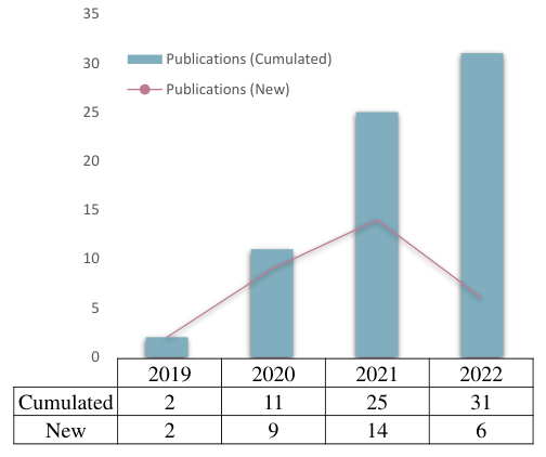
To understand how the concept of AutoML for deep recommender systems is implemented, we developed a comprehensive classification of existing methodologies. We do not claim to include all available research since our goals are to analyze different methods and determine their similarities or distinctions. The representative methods are selected from top computer science journals or conferences, such as KDD and WWW. The count of papers published per year is illustrated in Fig. 3. In this section, we describe the analysis questions, which determine our classification, and then our literature surveying procedure.
2.1. Analysis Questions
Our guiding question is how can the different components of the deep recommender systems be automatically designed to fit various scenarios and data. Under the guiding question, our survey paper focuses on the following three questions. (1) Which components of the models are automatically designed? (2) How is the compact search space designed so that it is general enough to include popular human-crafted models and not too general to prevent the success of the search for the new models? (3) How is the search algorithm designed so that exploration and exploitation can be balanced to enhance search efficiency and effectiveness?
2.2. Literature Surveying Procedure
To comprehensively answer the above analysis questions, we reviewed a wide range of papers discussing AutoML for deep recommender systems. A comparative and iterative literature review process is implemented. In the first round, a set of publications is inspected and summarized based on their answers to our analysis questions. We found that many papers automatically design the same component and encounter similar challenges. Therefore we classified those papers in the same category. The second round focuses on similar challenges within the same category and analyses the proposed methods to deal with similar challenges. In the third cycle, we sorted publications and enlarged our set of publications. Consequently, there is an extensive literature review where a distilled taxonomy includes various papers.

3. Backgrounds
3.1. Deep Recommender Systems
The frequently used notations are listed in Table 1. Deep learning has been widely applied to recommender systems because it captures the non-linear information and item-user relationships. Deep recommender systems (Meng et al. 2021) typically have four layers, as shown in Fig. 4: input layer, embedding layer, interaction layer, and prediction layer. We will give an introduction to the above components.
3.1.1. Input Layer
The input data usually contains three types of information, namely, the user profile (user ID, age, city, etc.), the item profile (category, item ID, etc.), and the context information (position, weekday, etc.) (Zhu et al. 2020). The input data for deep recommender systems is commonly in tabular format, i.e., numerical, categorical, or multi-valued features of multiple fields, as opposed to other forms of information like texts or images. The sample size of the tabular data is typically immense, with a highly sparse feature space (Cheng et al. 2016). It is common to apply one-hot or multi-hot encoding to map the raw features as binary features into high-dimensional feature space. For categorical feature field , binary feature is obtained by one-hot encoding. For numeric feature field, the numeric values are bucketed into discrete features manually (e.g. [0, 0, 0, 1] for ) or by training decision trees (e.g., GBDT (He et al. 2014)), and encoded as categorical feature field. Multi-valued fields are encoded by multi-hot encoding. The concatenation of binary features consists of a user-item interaction data instance (Zhao et al. 2021a):
where is the number of feature fields and is the binary vector for feature field.
3.1.2. Embedding Layer
The binary vectors are usually high-dimensional and sparse, which can be transformed into low-dimensional and dense vectors by feature embeddings. The embedding process is presented as follows:
For the binary feature generated from categorical or numeric feature field, feature embedding is obtained by:
| (1) |
where is the embedding matrix transforming the binary feature to condensed feature embedding . For feature field, is the size of pre-defined low-dimensional embedding and is the number of distinctive feature values.
For multi-valued feature field , is the embedding matrix. The embedding is obtained by:
| (2) |
where every feature is represented as a sequence, as the one-hot encoded binary vector, and is the maximal length of the sequence. The embedding can be aggregated to a dimensional vector by mean or sum pooling.
The output of embedding layer is the concatenation of all feature embeddings:
| (3) |
3.1.3. Interaction Layer
After the raw features are mapped in the low-dimensional space, an interaction layer is proposed to capture the feature interaction information between different feature fields. There are two types of feature interactions: explicit feature interactions and implicit feature interactions. Explicit feature interactions implement interaction functions among specific features, which are interpretable, and people acknowledge which features play an essential role in the model performance. Implicit feature interactions use multi-layer perceptron (MLP) to learn the non-linear information from all the feature embeddings.
Based on the convention definition (Lian et al. 2018), and the mathematical definition proposed in (Lyu et al. 2021), the result of explicit order of feature interaction is obtained by the feature embedding group :
| (4) |
where every in is searched from the concatenation of all feature embeddings , and is a feature interaction function, commonly designed by human experts. For example, Factorization Machines (FM) (Rendle 2010; Chen et al. 2020) implements the inner product of feature embeddings to explicitly model the order feature interactions, and define order interaction as the binary vector . In this scenario, the output of the interaction layer will be the output of FM:
| (5) |
where is the weight for binary vector , is the low dimensional feature embedding of field, and is the inner product of vector and vector . In theory, FM can explicitly model any order of feature interactions by the inner product of the corresponding feature embeddings. However, high order ( order with ) feature interaction introduces exponentially grown computation with respect to .
Multi-layer perceptron (MLP) can both learn the implicit feature interactions and integrate different orders of feature interaction and various types of embeddings, by extracting non-linear information with fully-connected layers and activation functions. The output of every layer is:
| (6) |
where is the activation function, is the weight, is the outputs of the previous layers, and is the bias. In many hand-crafted models, the output of MLP is combined with other embeddings before being taken as the output of the multi-interaction ensemble layer. DeepFM (Guo et al. 2017) concatenates the output of order feature interaction and the output of MLP on the embedding matrix, denoted as . IPNN (Qu et al. 2016) feeds explicit feature interactions and embedding matrix to MLP, and the output of feature interaction layer is denoted as .
3.1.4. Prediction Layer
The prediction layer yields the prediction based on the output of the feature interaction layer:
| (7) |
where is the weight, and is the bias. The specific recommendation task drives the choice of activation function . For instance, is preferred for the binary classification task (Guo et al. 2017), whereas is selected for multi-class classification (Song et al. 2019). The loss is calculated for the backpropagation steps based on the ground truth label :
| (8) |
where is the loss function, such as cross-entropy and mean-squared-error, usually determined by human experts (Zhao et al. 2021a).
3.2. Neural Architecture Search (NAS)
Neural Architecture Search (NAS) (Elsken et al. 2019; Pham et al. 2018) is proposed to search for the data-oriented and task-specific ideal deep learning architecture from the search space, alleviating considerable human effort in the architecture design procedure. Most works explore well-performed convolutional neural network architectures for different tasks like image classification (Chen et al. 2018a) and Natural language processing (Klyuchnikov et al. 2020). The NAS methods are determined by two significant factors: search space and search strategy. The set of all possible architectures is search space, which is broad enough to encompass existing well-performed architectures but still maintains a reasonable size to prevent increasing search costs. Within the search space, the search strategy efficiently searches for the preferred architecture and is expected to balance exploration and exploitation.
There are primarily three kinds of methodologies in the NAS field. (1) Sample-based approaches (Cai et al. 2018) explore new architecture by selecting from search space or mutating existing promising ones. (2) Reinforcement learning-based approaches (Liu et al. 2017; Real et al. 2017) implement a recurrent neural network as a policy controller to produce a sequence of actions to determine the architecture design. (3) Gradient-based approaches (Xie et al. 2018; Liu et al. 2018) convert the discrete search space to continuous and optimize the search architecture with the gradient descent calculated from the performance on the validation set. Differentiable Architecture Search (DARTS) employs continuous relaxation to search over the non-differentiable and discrete search space as a favored gradient descent-based NAS method.
3.2.1. Continuous Relaxation
Let represents the set of operations (e.g., the set of feature interaction candidate functions). To convert the search space continuous, a weight vector indicates the contribution of individual operation to the model performance, where , and is the number of positions waiting to be put a selected operation. The original one operation at position is replaced by the mixed operation with a softmax over all candidates (Maddison et al. 2016):
| (9) |
The task of searching for a well-performed discrete architecture with needed operations at positions is altered to jointly learn the architecture set , and the weight set of all operators. After learning procedure, the operator at position of the outputted discrete architecture is the one with the largest weight in the vector :
| (10) |
3.2.2. Gumbel-Softmax Operation
Like the above continuous relaxation, the Gumbel-Softmax operation substitutes a differentiable sample for the original non-differentiable categorical variable with a Gumbel-Softmax distribution (Jang et al. 2016). Thus stochastic neural networks can perform backpropagation through examples. Given the continuous distribution over the candidates, a hard selection is drawn by the Gumbel-Max trick (Gumbel 1954):
| (11) |
where are independent and identically distributed (i.i.d) noise samples drawn from and . However, the sampling is non-differentiable due to operation. The softmax function replaces as a continuous and differentiable approximation. Gumbel-Softmax generates , the probability of selecting the candidate as:
| (12) |
where is the temperature parameter that controls the smoothness of the operation. The Gumbel-Softmax operation’s output turns into a one-hot vector as gets closer to zero.
3.2.3. Bi-level Optimization
Similar to sample-based NAS (Cai et al. 2018) and reinforcement learning-based NAS (Liu et al. 2017; Real et al. 2017) using the model performance over the validation set as the fitness or reward, DARTS (Liu et al. 2018) utilizes the validation set to guide the learning procedure of and by optimizing the validation loss and training loss in a gradient descent manner. The output of NAS is acquired by minimizing the loss on the validation set, while the weight set is attained by minimizing the loss on the training set, which can be formulated as a bi-level optimization problem (Anandalingam and Friesz 1992; Colson et al. 2007):
| (13a) | ||||
| (13b) | ||||
where and represent the validation loss and training loss. is the upper-level parameter and is the lower-level parameter.
3.2.4. Architecture Gradient Approximation
After constructing the NAS problem as a bi-level optimization, DARTS introduces a straightforward approximation strategy to overcome the costly internal variable optimization in equation 13. Instead of solving the internal optimization entirely by training to convergence, is approximated by varying with one training step only (Liu et al. 2018). Thus this trick can also be called a one-step approximation:
| (14a) | ||||
| (14b) | ||||
where represents the learning rate for one step in the internal variable optimization, and indicates the contemporary weights acquired by the optimization. If reaches the local optimum for the internal optimization, and equation 14 degenerates to:
| (15) |
After the approximate architecture gradient is applied with the chain rule, it becomes:
| (16) |
where indicates the weights of the one-step forward model. accelerates the optimization procedure by neglecting the second order derivative, which is called first order approximation. Second order approximation refers to the scenario where . The choice of different approximation methods is the trade-off between accuracy and efficiency.
| Notations | Descriptions |
|---|---|
| set of users/items | |
| set of user-item examples | |
| set of feature interaction functions | |
| number of users | |
| feature field | |
| binary vector for feature field | |
| one user-item example | |
| feature embedding for binary vector | |
| vector of mixed embedding dimensions | |
| embedding matrix | |
| number of features fields | |
| pre-defined embedding dimension | |
| embedding dimension for feature field | |
| number of distinctive feature values for feature field | |
| pre-defined highest order for interaction | |
| Interaction between feature A and feature B | |
| element-wise product between and | |
| trainable weight | |
| feature interaction function | |
| activation function | |
| inner product of and | |
| loss function | |
| calculated loss value |
4. Automated Feature Selection Search (Auto-FSS)
As mentioned above, the input for deep recommender systems is binary vectors of feature fields. Most existing works (Guo et al. 2017; He et al. 2017) collect and use as many features as possible, regardless of whether the features are helpful for recommendation or not. This paradigm frequently calls for extra computations cost for feature embedding learning, additional inference time, and sub-optimal performance caused by the redundant or irrelevant features (Nadler and Coifman 2005). Therefore, selecting a subset of principal feature fields for deep recommender systems is highly demanded. The traditional feature selection methods such as hand-crafted by human experts, grid search (Glorot and Bengio 2010; Hinton 2012), or filter methods (Yu and Liu 2003) cannot be seamlessly integrated with deep recommender systems. For instance, filter methods omit the connection between subsequent models and feature selection. Therefore, automatically selecting features specifically as the input of recommendation models has attracted much attention in recent years, which is termed the automated feature selection search (Auto-FSS) in this paper. Auto-FSS faces the following two challenges. (1) Huge search space: Real-world recommender systems possess a vast number of unique features (e.g., more than a billion user IDs on YouTube) (Covington et al. 2016). These features and their cross features that are generated by operations over the unique features define the huge search space. Efficiently performing a search on the huge search space is a challenging problem. (2) Dynamic feature significance: In the recommendation tasks, the significance of a particular feature field may vary widely for different user-item interaction instances. Discovering the same useful feature subset for all instances limits the recommendation performance. It is worth mentioning that we only survey Auto-FSS for deep recommender systems as shown in Table 2, focusing on the above challenges since our main scope is AutoRecSys.
Methods Search Space Search Strategies Search Level Tasks AutoField (WWW’2022) (Wang et al. 2022) Gradient-based Raw Feature CTR AdaFS (KDD’2022) (Lin et al. 2022) MLP Raw Feature CTR GLIDER(ICLR’2020) (Tsang et al. 2020) Gradient-based Generated Feature CTR AutoCross (KDD’2019) (Luo et al. 2019) Beam Search Generated Feature CTR
AutoField (Wang et al. 2022) combines the feature selection process with the downstream recommendation tasks by implementing two-dimensional controller vectors to learn the contribution of each feature to the CTR prediction, where denotes the possibility of neglecting a feature filed, and represents the possibility of choosing a feature filed, , and . After parameters of controller vectors and deep recommender models are jointly learned by DARTS in a bi-level optimization manner, the Gumbel-Max trick simulates the hard feature selection process according to the controller parameters.
Following the idea of the controller in AutoField, AdaFS (Lin et al. 2022) provides an adaptive feature selection method for dynamic data instances rather than a static set. It utilizes a controller network with several fully-connected layers to output weights , revealing the importance of different feature fields for a data instance. Before the feature embedding is fed to the MLP as the input, BatchNorm (Ioffe and Szegedy 2015) is implemented to make the feature embedding with various magnitude comparable:
| (17) |
where represents a index for data instance in the batch, is a mini-batch mean, represents a variance, and is a small constant.
In addition to selecting relevant features from raw feature sets, some literature finds and produces useful combinatorial features (i.e., cross features), such as statistical features. GLIDER (Tsang et al. 2020) utilizes gradient-based Neural Interaction Detection (NID) (Tsang et al. 2017) to detect statistical feature interactions that span globally across multiple data instances from a source recommender model with a perturbation model called LIME (Ribeiro et al. 2016). Then, GLIDER explicitly encodes the generated features (i.e., searched global interaction) into a target recommendation model. The target recommendation model can be any classical recommender system, and the generated features are explored in search space.
AutoCross (Luo et al. 2019) enables feature selection from generated cross features, and performs the search in a tree-structured search space by implementing greedy beam search. It is different from feature interactions, as the output of AutoCorss is the useful feature sets, which can be fed to different recommendation models such as Wide&Deep (Cheng et al. 2016). The search space is tree-structured with the original feature set as the root and other nodes as the feature interaction set. If one node contains feature interactions, including original features, the number of children of that node is . Every child node is the parent node set, adding one feature interaction from the parent node set. The size of the search space is , growing exponentially with the maximum number of generated feature interactions .
To deal with the immense search space, the beam search, as a greedy strategy, is implemented in the tree-structured search space to traverse it from the root efficiently, by only exploring the most promising child node after evaluating all the children feature interaction sets for one node. In this greedy manner, it expands linearly with parameter , since only nodes will be evaluated in the search space.
In the feature set evaluation stage, field-wise logistic regression is applied to accelerate the process. It approximates the actual performance with mini-batch gradient descent. The model prediction is:
| (18) |
where and represent newly added interactive feature and features in the current set, respectively. Only the weight of the newly added feature interaction will be learned in the model training stage, while weights of current feature interactions stay fixed.
In the data processing stage, AutoCross proposes multi-granularity discretization, which discretizes one numerical feature with several levels of granularity rather than pre-defined granularity. It evaluates different discretized features, and only the best one is kept.
We analytically compare the above Auto-FSS methods as follows. AutoField and AdaFs search in the raw feature level within compact search spaces, while others search in the high-order generated cross feature level. There is no absolute winner among these two categories. Searching for raw features enables the task-specific subsequent recommender systems to discover the interactions and correlations within the original input features. It works well when the recommendation systems are expressive and have adequate computation resources. When the data distribution is rapidly changing in the scenario, or the significance of the high-order cross feature alters, the former is preferred since the downstream recommendation system can be finetuned, and the re-search procedure for the latter is time-consuming.
Within the raw feature search category, AdaFs selects different features for different data instances to address the second challenge, while AutoField outputs constant feature sets. Within the generated feature search category, AutoCross searches the explicit high-order feature interactions and can be fully deployed on the distributed systems to fit industrial needs. Both traditional recommender systems and deep neural models can be implemented after AutoCross constructs the feature interaction set. The drawback is also apparent. Exploring the high-order interaction feature space in a trial-and-error manner to prune the search pace leads to sub-optimal results.
5. Automated Embedding Dimension Search (Auto-EDS)

As mentioned above, the typical inputs of recommender systems involve many feature fields, and each field consists of a certain number of unique features ranging from a few to hundreds of millions. Since these original features are generally encoded as high-dimensional and sparse vectors, most modern deep recommender systems (Cheng et al. 2016; Covington et al. 2016; Rendle 2010; Guo et al. 2017) map them into the low-dimensional and dense feature representations (a.k.a., embeddings) for better capturing the implicit feature information. However, most of these methods assign a uniform embedding dimension for all features, suffering from the following issues. (1) Resources consumption: The huge number of parameters in the embedding matrix consume a large amount of storage and computational resources of the model. (2) Unappealing performance: The features generally follow a long-tail distribution in recommender systems (Park and Tuzhilin 2008), so setting the same dimension for head features and tail features may lead to sub-optimal performance. In particular, the high-frequency features need more parameters to express their rich information, and over-parameterizing the low-frequency features could cause overfitting due to the limited training data.
Thus, assigning embedding dimensions to each feature (field) automatically has attracted much attention in recent years, which is termed the automated embedding dimension search (Auto-EDS) in this paper. Concretely, as shown in Fig. 5, we introduce an overview of Auto-EDS architecture. The key component of Auto-EDS is the mixed dimension (MD) embedding layer, which consists of variable embedding sizes for each feature (fields). Then these MD embeddings are aligned into the same dimension via alignment operators (e.g., projection matrices (Ginart et al. 2021)) in the aligned embedding layer in order to satisfy the further operations (e.g., the dot product) in the interaction layer.
Existing methods in this research line could be categorized into heuristic, hyper-parameter optimization (HPO), and embedding pruning methods. We summarize these methods in Table 3.
5.1. Heuristic Methods
The heuristic methods generally assign embedding dimensions for each feature (field) based on the pre-defined human rules. For example, MDE (Ginart et al. 2021) introduces a mixed dimension (MD) embedding layer which assigns the embedding dimension based on the feature’s popularity. In particular, the MD layer consists of blocks corresponding to feature fields for the CTR task, and each block is defined by the embedding matrix and the projection matrix , respectively. The former stores embedding vectors for block (field) with dimension , and is the number of unique features in the field. The latter aligns the dimension into a base dimension for the further feature operations (e.g., the inner product) requiring consistent embedding dimensions. Thus, the question is how to assign mixed embedding dimensions for blocks. To this end, MDE first defines the block-level probability vector , and then the mixed embedding dimensions could be obtained as follows:
| (19) |
where is the hyperparameter controlling the degree of popularity influencing the embedding dimension.
Although such heuristic methods provided a simple scheme for assigning mixed embedding dimensions, the assumptions, i.e., the spectral decay following the power law, behind it were not guaranteed always to be satisfied, thus limiting its generalization on complex tasks.
5.2. HPO Methods
Inspired by the recent success of neural architecture search (NAS) (Zoph and Le 2016; Elsken et al. 2019) for automatically searching architectures for deep neural networks, another research line in Auto-EDS is to consider it as the hyper-parameter optimization (HPO) problem that searches embedding dimensions from a pre-defined candidate dimension set.
For example, NIS (Joglekar et al. 2020) (Neural Input Search) is the first HPO-based Auto-EDS work to automatically learn embedding dimensions and vocabulary sizes for each unique feature. In particular, it first sorts the unique features in decreasing order based on their frequency in the dataset resulting in a embedding matrix, where is the pre-defined maximum embedding dimension. Then, the is divided into a grid of submatrices (embedding blocks) with and , and the submatrix is of size such that and . In order to learn a MD embeddings, inspired by ENAS (Pham et al. 2018), a controller is employed to make a sequence of choices, and each choice is an , where means that the -dimensional embedding is removed. In this way, the search space size is , and the reward of the controller is defined by the combination of the quality reward (i.e., the metric values of the model evaluation on the validation set.) and the memory cost. Finally, the model is first trained by a warm-up phase to ensure that embedding blocks are expressive; after that, the main model (i.e., the recommendation model) and the controller are trained alternatingly by A3C (Mnih et al. 2016).
Inspired by the differentiable NAS (DARTS) (Liu et al. 2018), DNIS (Cheng et al. 2020) proposes a differential NIS framework to improve the search efficiency. Specifically, unlike NIS, which searches for embedding dimensions from pre-defined discrete dimension sets, DNIS argues that this restriction will hurt the flexibility of dimension selection and relax the search space to be continuous via the soft selection layer. In particular, for unique features, it uses binary dimension index vectors to maintain the ordered locations of the feature’s existing dimensions from the pre-defined dimension set , and then uses the similar feature sorting method as NIS to divide features into blocks such that features within the same block share the same binary dimension index vector. Thus, the total search space is . To learn efficiently, the is relaxed to be a continuous variable within the range of , named the soft selection layer, which is inserted between the embedding layer and the interaction layer. In this way, the relaxed dimension vectors could be jointly optimized with the embedding matrix by gradient descent. Furthermore, the gradient normalization operation is utilized to avoid numerical overflow. After training, the final output embedding matrix is obtained as follows:
| (20) |
where is the element-wise product. Finally, to obtain the MD embeddings, we could prune the by a pre-defined threshold.
AutoEmb (Zhaok et al. 2021) proposes an AutoML-based end-to-end framework in streaming recommendations that could automatically and dynamically select embedding dimensions for users/items based on their popularity changes. Specifically, each user and item are defined in the embedding spaces with embeddings ,, respectively, where are the corresponding embedding dimensions. Then, embeddings in different spaces are unified into the same space via the linear transform as follows:
| (21) |
where and are the weight matrix and bias vector, respectively. In order to make the magnitude of the transformed embeddings comparable, the Batch-Norm (Ioffe and Szegedy 2015) with the Tanh activation function (Karlik and Olgac 2011) is utilised to normalize the transform embeddings resulting in the magnitude-comparable user embedding vectors and item embedding vectors . Thus, the search space is , where and are the numbers of users and items, respectively. Furthermore, two MLP-based controller networks are used to choose dimensions from the above candidates for users and items based on their popularity and contextual information separately. In order to make the whole framework end-to-end differentiable, the soft selection layer that employs weighted sum of is utilised to obtain the final representations and of users and items as follow:
| (22) | ||||
where and are the weights for user representation and item representation,respectively. Finally, to jointly optimize parameters in embedding matrix and parameters in controllers, it introduces a variant of DARTS that leverage the first order approximation as equation 16.
AutoDim (Zhao et al. 2021b) extends the AutoEmb to the field-aware embedding dimension search, which aims to automatically assign embedding dimensions for different feature fields instead of users/items. In particular, similar to AutoEmb, each feature field is defined in the embedding space and then unified and normalized into the same space. The major difference is that it utilizes the Gumbel-softmax operation (Jang et al. 2016) with architecture weights to select embedding dimensions, which could also deal with the end-to-end indifferentiable issue due to the hard dimension selection. Finally, the DARTS-based optimization algorithm is also employed to optimize the embedding matrix and the architectural weights jointly.
Categories Methods Search Space Search Strategies Search Levels Tasks Heuristic MDE (ISIT’2021) (Ginart et al. 2021) — Human Rules Feature Fields CTR HPO NIS (KDD’2020) (Joglekar et al. 2020) ENAS-based Features Top-K Recommendation & CTR DNIS (ArXiv’2020) (Cheng et al. 2020) DARTS-based Features Rating Prediction & Top-K Recommendation & CTR AutoEmb (ICDM’2021) (Zhaok et al. 2021) DARTS-based Users/Items Rating Prediction AutoDim (WWW’2021) (Zhao et al. 2021b) DART-based Feature Fields CTR ESAPN (SIGIR’2020) (Liu et al. 2020b) ENAS-based Users/Items CTR & Rating Prediction Embedding Prunning PEP (ICLR’2021) (Liu et al. 2021) — Soft Threshold Reparameterization Features CTR AMTL (CIKM’2021) (Yan et al. 2021) — Adaptively-Masked Layer Features CTR RULE (KDD’2021) (Chen et al. 2021) Evolutionary Search Items Top-K Recommendation DeepLight (WSDM’2021) (Deng et al. 2021) — Greedy Algorithm Features/DNN CTR SSEDS (SIGIR’2022) (Qu et al. 2022) — Dimension Salience Criterion Feature Fields CTR
ESAPN (Liu et al. 2020b) aims to search embedding dimensions for users and items dynamically based on their popularity by an automated reinforcement learning agent. However, unlike AutoEmb using a soft selection strategy, ESAPN performs a hard selection on candidate embedding dimensions, which could effectively reduce the storage space. Specifically, it consists of a deep recommendation model performing personalized recommendations and two policy networks learning embedding dimensions for users and items from a discrete candidate dimension set. The deep recommendation component is similar to AutoEmb which the embeddings of users/items are defined in various embedding spaces and then are transformed into the largest dimension via linear transformations and batch normalization. For policy networks which are multi-layer perceptrons with multiple hidden layers, they take the frequency and current embedding dimension of users/items as inputs (i.e., states for reinforcement learning agent) and output two possible actions: enlarging the current dimension to the next larger dimension or unchanging the current dimension. The design of such actions is because they assume that users/items with a higher frequency have larger embedding dimensions. Furthermore, the reward of policy networks is defined based on the difference between the current prediction loss and the previous losses. Finally, inspired by ENAS (Pham et al. 2018), the recommendation model and policy networks are optimized in an alternative fashion, which optimizes policy networks using the sampled validation data and uses training data to optimize the recommendation model.
Although HPO-based Auto-EDS methods could effectively learn MD embeddings in different levels (i.e., features, feature fields, and users/items), such kinds of methods still suffer from several issues. (1) Resources consumption: to maintain embeddings on different embedding spaces (Zhaok et al. 2021; Zhao et al. 2021b; Liu et al. 2020b), they have to maintain additional embedding matrixes with different dimensions, which consumes a huge amount of storage space. (2) Expensive optimization: the model overall model optimization is time-consuming due to optimizing the extra parameters in controllers (Liu et al. 2020b; Joglekar et al. 2020). (3) Severe assumption: the assumption that the high-frequency features (users/items) should be assigned with the larger embedding dimensions (Liu et al. 2020b; Joglekar et al. 2020) might not always be satisfied due to the complex situations in recommendations.
5.3. Embedding Pruning Methods
Another research line in this field considers the Auto-EDS as the embedding pruning problem, which performs embedding pruning over the whole embedding matrix using different pruning strategies such that the MD embeddings are automatically obtained. Thus, the key idea of such kinds of methods is to build memory-efficient models by identifying and removing the redundant parameters in the embedding matrix and keeping the recommendation as accurate as possible.
For example, PEP (Liu et al. 2021) introduces the learnable thresholds to identify the importance of parameters in the embedding matrix. In particular, inspired by Soft Threshold Reparameterization (Kusupati et al. 2020), it directly performs adaptively pruning as follows:
| (23) |
where and are the re-parameterized embedding matrix and original embedding matrix, respectively. is the absolute operation. is learnable threshold(s) that could be updated by gradient descent, and is sign function. Furthermore, the sub-gradient is utilized to solve the non-differentiability of equation (23) as below:
| (24) |
where denotes -th step learning rate, and is element-wise product. and are the loss function (e.g., the cross-entropy loss) and the dataset, respectively. is the indicator function. In this way, the threshold(s) and embedding matrix could be jointly trained by gradient descent. After that, it could mask those dropped parameters in to obtain a pruned embedding matrix which could be utilized to re-train the based model according to the Lottery Tickey Hypothesis (Frankle and Carbin 2018).
ATML (Yan et al. 2021) proposes to use an Adaptively-Masked Twins-based layer (i.e., AMTL) behind the original embedding layer to learn a mask vector which is utilized to mask those redundant dimensions in the embedding matrix. Specifically, to leverage the feature frequency knowledge, the AMTL takes the feature frequency vectors as input and then uses two branches (i.e., h-AML and l-AML) to handle high-frequency and low-frequency samples, respectively, so that the parameters in l-AML will not be dominated by the high-frequency samples. Moreover, it introduces a soft decision strategy to determine the high- or low- frequency samples, which uses a weighted sum of outputs of h-AML and l-AML as follows:
| (25) | ||||
where and are the -th outputs of l-AML and h-AML, respectively, and is the weight which is influenced by the feature frequency . Then, a temperated softmax function (Hinton et al. 2015) is applied on to obtain the probability to select different embedding dimensions.
RULE (Chen et al. 2021) proposes an on-device recommendation paradigm with elastic embeddings dealing with various memory budgets for devices. The paradigm is divided into learning full embeddings and searching elastic embeddings for items with an evolutionary algorithm. As argued by the authors, the learning time of embedding is far beyond the searching time, leading to a once-for-all paradigm, which adapts the learned embedding table to local on-device recommenders with heterogeneous resource budgets. In the learning phase, Bayesian personalized ranking (BPR) (Rendle et al. 2012) loss is applied to optimize the full embedding and regularization terms maintaining the diversity of the learned embedding blocks, benefiting the subsequent search procedure. In the deployment phase, the evolutionary algorithm (Real et al. 2019) with a single-layer feed-forward network estimator is adopted to search the desired embedding blocks under the memory budgets. The search space is , where the hyper-parameters , represent the number of embedding blocks for an item, and the number of item groups respectively. The embedding pruning is done by maintaining the searched embeddings by evolutionary algorithms.
Deeplight (Deng et al. 2021) proposes to prune both parameters in the embedding layer and DNN layer to solve the high-latency issues in CTR prediction. The weight matrices of the DNN component are pruned to remove the connections. Thus, the sparse DNN component with less computation complexity contributes to the training acceleration. The field pair interaction matrix is pruned as field pair selection. Moreover, the elements in the embedding vectors are pruned to be sparse embedding vectors. Considering the majority of the parameters in deep learning models for click prediction are feature embeddings, Deeplight is classified into Auto-EDS in our taxonomy. The model is trained for a few epochs, and weights with the smallest values are removed based on adaptive sparse rate. The search strategy can be summarized as the variant of the greedy algorithm with weak sub-modular optimization (Das and Kempe 2011).
SSEDS (Qu et al. 2022) proposes a single-shot embedding pruning method named SSEDS. In particular, it first pre-trains a traditional CTR model with unified embedding dimensions, and then utilizes the proposed criterion which could measure the importance of embedding dimensions only in one forward-backward pass to obtain the salience scores of each dimension. In this way, the redundant dimensions could be removed based on the dimension importance ranking and the parameter budget. Furthermore, since the obtained mixed-dimensional embeddings could not be directly applied to traditional CTR models due to some feature interaction operations (e.g., the dot product) requiring all embeddings with the same dimension, SSEDS utilizes the additional transform matrices to align all dimensions and re-trains the slim model.
Although the embedding pruning-based Auto-EDS methods could build the memory-efficient model via selectively reducing parameters in the embedding matrix, these methods generally require an iterative optimization procedure for both parameters in the embedding matrix and additional parameters used to prune, which is time-consuming.
6. Automated Feature Interaction Search (Auto-FIS)

Feature interactions combine individual features of users, items, and other context information. For instance, the user’s age and generic of the downloaded application can be combined together as the order feature interactions and contribute to the users’ preference prediction in the application recommendation scenario. The order implements the number of combined features. The effectiveness of order feature interactions has been proved in Factorization Machines (FMs) (Rendle 2010) and their variants (Pasricha and McAuley 2018)(Juan et al. 2016). Meanwhile, the high-order ( order with ) feature interactions is approximated by Higher-order Factorization Machine (HOFM) (Blondel et al. 2016).
With the prosperity of deep neural networks, many deep learning recommender models have been proposed due to their better performance than traditional models. Product-based Neural Network (PNN) (Qu et al. 2016) extracts the high-order feature interactions and discards the lower ones. Wide&Deep (Cheng et al. 2016) and DeepFM (Guo et al. 2017) learn the low-order and high-order feature interactions by a shallow component and a deep component and state that both the low-order and high order feature interactions play a significant role in context-aware recommender systems.
However, enumerating all high-order feature interactions is time and space-consuming. When there are features in total, the number of order interaction terms is . Even for order feature interactions, simply listing all combinations may introduce useless interactions as noise and disturb the model performance. Therefore, how to keep the necessary feature interactions and filter out the useless ones arouse people’s interest. We summarize these methods in Table 4. Many automated feature interaction search methods are proposed to deal with the following three challenges mainly. (1) The desired beneficial feature interaction sets are discrete. (2) Both lower and higher order feature interactions are highly correlated. (3) The priorities of the low- and high-order interactions in the search procedure should be considered. Concretely, as shown in Fig. 6, we introduce an overview of Automated Feature Interaction Search (Auto-FIS) architecture. The key components are the set containing all possible order feature interactions and the discarded connections, which are determined by the search procedure.
Sparse Factorization Machines (SFMs) (Zhao et al. 2017) determine the relevant user features and item features based on their contributions to the prediction model by sparsity regularization (Tibshirani 1996). If one feature does not contribute to the predictive modeling, entire feature interactions related to it will be deactivated. If some significant high-order feature interactions play a role in the prediction only as a whole rather than individuals, SFMs may discard them even it has a recovery procedure to cover features that are relevant to user-item prediction. Moreover, the feature interaction selection strategy of SFMs is identical for all users. Same interactions may play a more important role to one user than others. The most intuitive solution is to build distant SFMs for every user, which does not preserve the benefit of collaborative filtering.
Thus, Bayesian Personalized Feature Interaction Selection (BP-FIS) (Chen et al. 2019) is proposed to adaptively select interactions for individual users by Bayesian Variable Selection (Mitchell and Beauchamp 1988). The prediction is modified as below:
| (26) |
where is the bias for user . The single feature interaction weights are learned for all users, while personalized feature interaction selection variables indicate the order and order feature interaction selection for individual user . is the number of users. Due to the immense search space , BP-FIS proposes Hereditary Spike-and-Slab Prior (HSSP) based on Spike-and-Slab Priors (SSPs) (Bernardo et al. 2003) to attain the heredity property of feature interaction. Strong heredity indicates that if the order interactions and are chosen, their combination, i.e., the order interaction would be selected, while weak heredity indicates the selection possibility of their combination to be when only one of the order interactions is selected. To be specific, the HSSP is stated as:
| (27) | ||||
where are constant values. Inspired by Variational Auto-Encoder (VAE) (Kingma and Welling 2013), Stochastic Gradient Variational Bayes (SGVB) estimator is proposed to approximate posteriors of the latent variables and optimize the model. BP-FIS can be combined with both linear FM and neural FM.
AutoFIS (Liu et al. 2020c) is proposed to learn the feature interactions in recommender system models by adding an attention gate to every potential feature interaction, rather than simply enumerating all the two-order feature interactions like Factorization Machines. There are two stages for AutoFIS: the search stage and the re-train stage.
In the search stage, equation 28 shows the interaction layer of the factorization model in AutoFIS.
| (28) |
Instead of searching the desired discrete combination set from search space for two-order feature interactions, the wight represents the importance of the interaction between vector and vector , and determinates whether preserve or delete this interaction. After feeding the output of the interaction layer as the input of multi-layer perceptron (MLP), the user’s preference for item can be calculated via:
| (29) |
Architecture parameters reveal the contribution of every feature interaction towards the final prediction. Furthermore, the architecture parameters are trained by generalized regularized dual averaging (GRDA) optimizer (Chao and Cheng 2019), while other parameters (such as in equation 28 ) are updated by Adam optimizer (Kingma and Ba 2014). These two optimizations are conducted jointly in one gradient descent step, unlike the bi-level optimization algorithm in DARTS (Liu et al. 2018).
In the re-train stage, architecture parameters are fixed as after search stage. Feature interactions that benefit the final prediction have higher values. The feature interaction layer in equation 28 is modified as:
| (30) |
where depicting the gate status is set as 0 when = 0, otherwise 1. With attention unit , the model is further trained by relative important interactions, and all the parameters are learned by Adam optimizer (Kingma and Ba 2014).
Unlike AutoFIS simply focusing on two-order feature interaction selections, AutoGroup (Liu et al. 2020a) considers the high-order feature interaction search as a structural optimization problem to identify the useful high-order interactions. The search space is , where pre-defined represents the maximum order of feature interactions. Firstly, for order of feature interactions, it selects feature sets. represents the feature set for order. Every feature is possible to be included in indicated by the structural parameter .
After the automatic feature grouping stage, the representation of a feature set is defined as the weighted sum of feature embedding within it:
| (31) |
where is the embedding of feature and is trainable weight parameter. Inspired by FM (Rendle 2010), the time complexity is reduced from to , owning to feature interaction calculation method within one feature set .
| (32) |
where represents the sum of all the embedding components of the embedding generated by times the element-wise product of with itself. There are interaction results in total. All the interactions are concatenated and fed into an MLP. The prediction is calculated by:
| (33) |
AutoGroup optimizes the structural parameters and network weights (e.g., embedding parameters and MLP parameters) alternatively by gradient descent, similar to DARTS (Liu et al. 2018), since two kinds of trainable parameters are highly dependent on each other.
Methods Search Space Search Strategies Order Tasks BP-FIS (SIGIR’2019) (Chen et al. 2019) Bayesian Optimization Explicit Low Order Top-K Recommendation AutoFIS (KDD’2020) (Liu et al. 2020c) Gradient-based Explicit Low Order CTR AutoGroup (SIGIR’2020) (Liu et al. 2020a) Gradient-based Explicit High Order CTR FIVES (KDD’2021) (Xie et al. 2021) Gradient-based Explicit High Order CTR FROFIT (NeurIPS’2021) (Gao et al. 2021) Gradient-based Explicit High Order CTR -SIGN (AAAI’2021) (Su et al. 2021) MLP Explicit Low Order CTR HIRS (KDD ’2022) (Su et al. 2022) MLP Explicit High Order Top-K Recommendation
With the prosperity of Graph Neural Network (GNN), -SIGN (Su et al. 2021) implements GNN techniques to tackle the feature interaction search problem. Given a Graph , where represents feature , edge from the edge set represents whether select the feature interaction between feature and feature . Initially, the edge set is empty , and the task of searching for beneficial feature interactions is converted to the edge prediction in graph . Therefore, the complexity of the search space is . -SIGN implements an MLP to predict the edge:
| (34) |
where the feature embedding and are obtained by equation 1 and 2. Set including all detected edges , is performed with an activation regularization to minimize the number of searched beneficial interactions. After determining the edge set , the embedding is updated iteratively times by a linear aggregation function (e.g. element-wise summation/mean):
| (35) |
where is the iteration index, and is the set of statistical interaction analysis outcomes between (i.e. the embedding of node at iteration) and embeddings of its neighbours. The final prediction is calculated as:
| (36) |
where the linear function (e.g., weighted sum function) converts the node embedding to a scalar value, and is the bias term.
While -SIGN can only search for the -order feature interaction, HIRS (Su et al. 2021) extends it to arbitrary order of feature interaction by introducing the hyper-edge set , where hyper-parameter represents the number of intended search feature interaction. Each hyper-edge is -dimensional binary vector , where represents that the hyper-edge links to feature . The hyper-edge prediction module contains a multi-layer perceptron, looking through the search space with complexity .
Under the same settings of graph , FIVES (Xie et al. 2021) extends the interaction search to high-order with a graph neural network and an adjacency tensor. Adjacency tensor indicates the interactions at every order . is the representation for node at order , and . Based on the proposition that the interaction of uninformative ones is unlikely to build an informative feature, when is active, is calculated as:
| (37) |
where "MEAN" is the aggregator, is the element-wise product, and represents the transformation matrix for node . Under the assumption that can express feature interaction , the node representation matches the order feature interactions, and adjacency tensor determines which features to be selected. Thus, the search space is .
The search problem of FIVES is a Bi-level optimization where is the upper-level variable, and other model variables are the lower-level ones,
Following the settings in AutoFIS, where gradient descent NAS method with relaxation turns the search space into symmetric parameter matrix , PROFIT (Gao et al. 2021) finds that parameter matrix has several dominant singular values, and exhibits a low-rank property. Therefore, PROFIT proposes a distilled search space by symmetric CP decomposition (Kolda and Bader 2009), extending to order interactions:
| (38) |
where approximated vector is updated by gradient descent, and the distilled search space is based on low-rank approximation with a positive integer . The authors state that the complexity is . Following the idea that different orders of feature interactions are highly correlated, PROFIT proposes a progressive gradient descent to learn the high-order after the low one. Specifically, when learning the order interaction, the architecture parameters are fixed.
BP-FIS has two major drawbacks. (1) BP-FIS limits the interactions up to two orders. (2) Selection for every user may be a waste of resources. Group-level penalization could be an efficient manner to control the size of the search space.
AutoFIS, AutoGroup, and AutoCross adopt NAS on the continuous search space with the help of continuous relaxation. The search problem is modified from choosing one interaction to calculating the weight of that interaction. The complexity of search space is reduced from the original search space to the number of the weight parameters . However, they still encounter several issues. (1) Slow optimization procedure: The number of weight parameters is significantly greater than existing gradient-based NAS methods (Liu et al. 2018; Xie et al. 2018), which usually have less than one hundred parameters. (2) Ignorance on the order-priority property: They neglect the relations between different order interactions.
Both implementing GNN techniques to search for beneficial feature interactions, -SIGN focuses on order feature interactions. In contrast, FIVES extends to high-order under the proposition that it is improbable to produce the instructive feature interactions from the uninformative interactions, which may miss particular significant interactions in some scenarios. Although the search space of PROFIT has been dramatically reduced, the choice of hyper-parameter influences the final performance.
Methods Search Space Search Strategies Tasks AutoCTR (KDD’2020) (Song et al. 2020) Multi-Objective Evo CTR AMEIR (IJCAI’2021) (Zhao et al. 2021c) One-shot Random Search CTR AutoIAS (CIKM’2021) (Wei et al. 2021) MLP CTR NASR (WWW’2022) (Cheng et al. 2022) Greedy Search Top-K Recommendation
7. Automated Model Architecture Search (Auto-MAS)
Numerous classical approaches (Lian et al. 2018; Wang et al. 2017) have demonstrated the significance and effectiveness of feature interactions in coping with high-cardinality feature attributes and large-scale datasets. They discover the explicit low-order feature interactions and combine them with explicit or implicit high-order feature interactions. For instance, Wide&Deep (Cheng et al. 2016) and DeepFM (Guo et al. 2017) learn the explicit low-order and implicit high-order feature interactions by a shallow and a deep component. The section on feature interaction search methods systematically reviews various techniques to identify beneficial feature interactions. However, existing methods search for one particular layer and leave other components of the deep recommender systems hand-crafted, causing three problems. (1) An integrated recommender system model cannot be directly obtained by the above-mentioned automated search methods, and domain experts are needed to design other components manually. (2) An whole well-performed architecture is less likely to be acquired due to other hand-crafted components, even the searched one finding the best candidate. (3) The generalization capacity is decreased by the limited search space for one specific layer rather than the whole architecture.
Moreover, the design of MLP layers in classical approaches may not be optimal both in efficiency and effectiveness. Diamond MLP frameworks may outperform rectangular, and triangle frameworks (Zhang et al. 2016), which aroused people’s interest in the MLP design. Experts cannot attempt all the potential design architecture. Therefore, automated model architecture search methods are employed to mitigate human efforts and search for an automatically designed task-specific architecture that organically combines informative embeddings and various feature interactions. There are mainly three challenges. (1) Accurate search space: The search space of automated model architecture search methods should be carefully designed, which includes popular and effective human-crafted architectures. In the meantime, the search space cannot be exceedingly general. (2) Search Efficiency: Automated model architecture search methods should be efficient, especially for the design of the recommender system architecture. A practical model encounters a billion-level of user-item data in the industry, for example, the private dataset in AutoFIS (Liu et al. 2020c) from Huawei App Store. (3) Ability to distinguish: Recommender systems with diverse architecture may lead to similar performance on the validation dataset since minor improvements to the experiment contribute to significant refinements in practice. Automated model architecture search methods should be sensitive to slight progress. We summarize these methods in Table 5.
AutoCTR (Song et al. 2020) proposes a two-level hierarchical search space, which includes the popular human-crafted deep recommender system architectures by abstracting different feature interaction methods into virtual blocks. The inner search space contains the choice of virtual blocks and detailed hyperparameters inside each of those blocks. Based on the existing literature, the virtual blocks can be selected from FM, MLP, and dot products. Instead of simply stacking the blocks sequentially, AutoCTR implements a direct acyclic graph (DAG) to connect different feature interaction blocks organically, rather than directly stacking different components sequentially. A block may receive outputs from any preceding block, including numerous unexplored architectures. The outer search space contains all the possible block combination choices. Let represent the number of virtual blocks, controlling the complexity of the architectures. There are four basic candidate operators for blocks, and possible connections for blocks. Therefore the search space is .
A multi-objective evolutionary search is used to explore the two-level hierarchical search space. The first procedure is survivor selection. Only top- architectures survive according to the metric :
| (39) |
where is the hyperparameter larger than , and the indicator function filters out architectures older than q. Three objectives of the architecture : age , performance , and complexity are balanced by parameters , , and . To tackle the third challenge mentioned above, the probability of being selected as the parents in the second procedure is denoted as:
| (40) |
where hyperparameter balances exploitation and exploration. In the last procedure, a learning-to-rank strategy is adopted to guide the mutations by the gradient boosted tree learner and a pairwise ranking loss named LambdaRank (Burges 2010).
AMEIR (Zhao et al. 2021c) divides the recommendation models into three stages: behavior modeling, feature interaction, and MLP aggregation. Behavior modeling networks encapsulate users’ specific and dynamic interests based on the sequential input features. Behavior modeling networks have three components: normalization, specific layer, and activation function, respectively selected from three candidate sets: {layer normalization, None}, {convolutional, recurrent, pooling, attention}, {ReLU, GeLU, Swish, Identity}. The search subspace of feature interactions is , containing all possible combinations of order feature interactions. For the MLP aggregation stage, the number of hidden units has ten candidate values, and the activation function is chosen from {ReLU, Swish, Identity, Dice}. Therefore the complexity of the overall search is , where and represent the number of layers for behavior modeling and MLP respectively.
A one-shot random search is implemented to incorporate industrial requirements rather than a one-shot weight-sharing paradigm. It randomly samples child models from the search space and reserves the one with the best performance on the validation set. By gradually increasing the order of interactions, effective feature interactions are discovered. Beneficial interaction set with the fixed size is initialized with feature matrix and updated by interacting with . New interactions with the highest validation fitness are retained in the interaction set.
AutoIAS (Wei et al. 2021) provides a more fine-grained search space including six components with number of candidates, where . First component represents the embedding size for each binary feature vector . determines the unified projection embedding size before interaction for every order interaction pair, and the third component decides the feature interaction function. inserts the result of one interaction into the layer of MLP to mix the low- and high-order of feature interactions. The input of layer is the concatenation between the interaction result and the output of layer. The output of layer is calculated as:
| (41) |
where . decides the number of layers in MLP. AutoIAS implements architecture generator network to search through the immense search space with complexity . The Deep Neural Network (DNN) models the dependencies among different components by taking in previous components’ states and generating the current component’s selection probability on the candidate set. The performance prediction of a particular architecture is fastened by the ordinal parameter sharing on the supernet whose embedding size for different components is the largest one over the corresponding candidate set.
Unlike the above methods, NASR (Cheng et al. 2022) is an Auto-MAS model, searching hybrid architectures for the sequential recommendation. To alleviate the dilemma where increasing the number of depth layers leads to difficult training for neural networks (He et al. 2016), NASR adds one trainable parameter to the residual connection:
| (42) |
where and indicate the input and output for -th residual block. is the learnable residual mapping, and represent all the parameters for -th block. The trainable parameter boosts convergence and improves sequential recommendation performance. The search space consists of deep layers. For each layer, there are four candidates: two transformer block variants, and two temporal convolutional network variants. A greedy search strategy is utilized, accompanied by an unsupervised evaluation metric, which estimates the performance for each candidate layer.
One of the biggest challenges in automated model architecture search is the immense search space. All three methods suffer from this issue and propose distinct solutions to deal with it. AutoCTR implements multi-objective evolutionary search rather than gradient descent methods to parallelly explore the vast search space. AMEIR employs a one-shot random search to accelerate the search process, while AutoIAS utilizes DNN to model the dependencies among different components. Although the automated model architecture search is appealing and directly outputs well-performed recommender systems, simply stacking all the possible candidates leads to huge search space and is not practical in real-world applications. The inner relation between different components should be discovered, or some rule should be implemented to shrink the search space and serve as a search strategy guideline.

8. Automated Other Components Search (Auto-OCS)
8.1. Loss Function Search
Deep neural networks (DNN) show promising results in recommender systems. One pivotal part of DNN training is the backpropagation, calculating the gradient based on the pre-defined loss function. However, choosing distinct loss functions is not universal and does not guarantee good performance. More appropriate gradients with a carefully-designed loss function may contribute to a better deep model.
People manually designed loss functions for specific tasks and purposes. A loss function with a higher value at the boundary position is proposed to improve the boundary metrics and satisfy the scenario when the boundary region is more significant (Qin et al. 2019). A large-margin softmax loss function in the image processing field is proposed to replace the common softmax loss function for desired feature discrimination learning (Liu et al. 2016).
Despite the effectiveness of manually-designed loss functions, the exhausting design process requires human experts and a heavy workload. As shown in Fig. 7, the automated loss search method selects the proper loss function concerning different tasks and goals from the set of loss function candidates.
Given a set of loss function candidates with size , the complexity of search space is . Stochastic loss function (SLF) (Liu and Lai 2020) calculates the overall loss value as follows:
| (43) |
where a set of weights represents the contributions of individual loss functions, while and represent the ground truth and prediction, respectively. However, this soft fusing strategy cannot prohibit the sub-optimal loss function from depreciating the loss value . To tackle this problem, AutoLoss (Zhao et al. 2021a) simulates the hard selection with Gumbel-softmax operation on the weight set . Moreover, diverse user-item interaction examples exhibit different convergence behaviors. The weight set for every example cannot be initialized by the same static probability. AutoLoss uses a controller network with several fully-connected layers like equation 6, taking the pair as input and outputting the weight set. Therefore, the weight set is adaptively produced for different examples depending on distinct convergence behavior patterns.
Although seldom works implement loss function search in recommendation scenario. Automated loss function search itself is not a brand new field direction. In the image semantic segmentation application, AUTO SEG-LOSS (Li et al. 2020) searches particular surrogate losses and enhances the model performance on distinct metrics. In the face recognition task, a search space and a reward-guided search method (Wang et al. 2020b) are presented to acquire the best loss function candidate. Those papers validate the effectiveness of the automated loss function search. Perhaps some methodologies can be transferred to recommendation tasks, or new methods can be explicitly proposed for recommendation scenarios. The training efficiency of recommender system models can be further improved.
Categories Methods Search Space Search Strategies Tasks Loss Function Search AutoLoss (KDD’2021) (Zhao et al. 2021a) MLP CTR & 5-star ratings Feature Interaction Function Search SIF (WWW’2020) (Yao et al. 2020a) Gradient based Top-K recommendation OptInter (ICDE’2022) (Lyu et al. 2021) Gradient based CTR AutoFeature (CIKM’2020) (Khawar et al. 2020) Naive Bayes tree CTR AutoPI (SIGIR’2021) (Meng et al. 2021) Gradient based CTR
8.2. Feature Interaction Function Search
The effectiveness of feature interaction has been addressed in recent techniques, and various search methods for beneficial interactions are introduced above. However, most literature uses the same feature interaction function to model all the feature interactions while neglecting their distinction. Wide&Deep (Cheng et al. 2016) implements a shallow component and MLP to model low- and high-order interactions. Attention networks distinguish the contributions of order interaction in AFM (Xiao et al. 2017) and DIN (Zhou et al. 2019a). Only simple inner product operations are employed in PNN (Qu et al. 2016) and DeepFM (Guo et al. 2017). PIN (Zhang et al. 2016) presents a net-in-net architecture to model the pairwise interactions, accompanied by a product-based neural network. All the literature mentioned above implements the same network architecture or inner product to learn interactions regardless of the input data change, which leads to sub-optimal performance. Therefore, feature interaction search methods are needed to search for suitable interaction functions according to different datasets and tasks as shown in Fig. 7. We summarize these methods in Table 6.
Simple neural interaction functions (SIF) (Yao et al. 2020a) has been proposed to automatically select interaction function for collaborative filtering (CF) (Koren et al. 2022). Within the search space, interaction function between user and item is designed as . is the simple non-linear element-wise operation (small MLP with fixed architecture) and is the vector-wise operations selected from five candidates. Let denote the number of selected operations. The search space is , including popular human-designed interaction functions. Moreover, inspired by an efficient NAS method based on proximal iterations (NASP) (Yao et al. 2020b), SIF implements a one-shot search algorithm jointly searching interaction functions and updating the learning parameters through stochastic gradient descent.
Unlike SIF searches proper functions for all feature interactions. OptInter (Lyu et al. 2021) divides the potential feature function into three categories for every order feature interaction: element-wise product, MLP, and memorized methods, which regard interactions as a new feature and assign trainable weights. There are three function candidates for each interaction, and order feature interactions exist. Therefore, the complexity of the search space is . The element-wise product for and is represented as:
| (44) |
Gradient descent-based NAS search method with Gumbel-softmax operation is implemented to make the discrete search space continuous, and the architecture parameters can be learned by Adam optimizer (Kingma and Ba 2014).
AutoPI (Meng et al. 2021) introduces the computational graph to search space. The computational graph is a directed acyclic graph (DAG) comprising input nodes, intermediate nodes, and the output node in an ordered sequence. is the pre-defined parameter that controls the complexity of the computational graph. Every node contains a feature matrix stacked by feature embeddings with size , and every directed edge between node and node represents an interaction function , which transforms the feature matrix . Every intermediate node is calculated using all of its predecessors’ values:
| (45) |
There are edges, and for each edge, one interaction function is searched from an interaction function set , including six candidates. Therefore, the search space is . Six feature interaction functions candidates are Skip-connection, SENET layer (Huang et al. 2019), Self-attention (Song et al. 2019), FM (Rendle 2010), Single-layer Perceptron, and 1d Convolution. Skip-connection outputs the same feature matrix as the input. Single-layer Perceptron uses a linear transformation to transform a flattened feature into a feature matrix , and 1d Convolution outputs a feature matrix through kernel matrices.
In the search stage, inspired by DARTS (Liu et al. 2018), a gradient descent NAS method converts the combinatorial search problem to a bi-level optimization with continuous relaxation. Node-level parameters show the weights of different interaction functions, where is a vector with size . Since the value of one node is determined by all its predecessors, edge-level weights represent the contributions of the node to the node , where is a scalar. The bi-level optimization is formulated with as the upper-level parameters and other weights as the lower-level parameters. The one-step approximation (Liu et al. 2018) is implemented to tackle the expensive inner optimization problem by approximating the architecture gradient.
AutoFeature (Khawar et al. 2020) extends the search of proper interaction function for every interaction to high-order with a distinct DAG sub-network structure. The DAG contains a pre-defined number of operations selected from five interaction functions: pointwise addition, Hadamard product, concatenation, generalized product, and none. The search space is , where represents the number of operations in the sub-network, represents the number of features, and represents the interaction order. Due to the immense search space, a tree of Naive Bayes classifiers (NBTree) with thresholds indicating the percentile of explored space partitions the search space of architectures recursively. As for the search strategy, the likelihood of selecting from a node is proportionate to the number of samplings formerly selected from that node.
SIF (Yao et al. 2020a) chooses the proper feature interaction function for all order interactions while neglecting that different feature interactions may require different methodologies to model. Based on SIF, AutoFeature (Khawar et al. 2020) searches individual functions for every interaction and extends the order of interactions, including most interaction modeling techniques, but high-order interaction and complex DAG components lead to immense search space. Besides, the search strategy of AutoFeature (Khawar et al. 2020) can be trapped in the local optimal. OptInter (Lyu et al. 2021) balances the efficiency and the generalization of the search space, searching distinct functions for every interaction limited to order, and introduces memorized methods as the candidate of feature interaction functions. Taking feature interactions as new features benefits the model performance since this action makes the correlated patterns of some interactions with strong signals more accessible to be captured. It is worth mentioning that the abuse of memorized methods may depreciate the overall performance due to the overfitting problem accompanied by sparse new features.
9. Horizontal Comparison for AutoRecSys
The empirical analysis aims to help practitioners investigate the bottlenecks and strengths of current AutoRecSys models from different aspects (e.g., number of parameters, training time, etc.). Then researchers can evaluate the applicability of the existing method to their unique problems or scenarios. Therefore, we select the representative AutoRecSys methods to perform the empirical analyses for two tasks: click-through prediction (CTR) and Top-K recommendation.
9.1. Experiment details and hyper-parameter setting
Following the experiment settings in the original papers, we employ commonly-used metrics, Recall@10 (i.e., recall at rank 10) and NDCG@10 (i.e., normalized discounted cumulative gain at rank 10) for Top-K recommendation, and Area Under the ROC Curve (AUC) for click-through prediction (CTR). To gauge the complexity of the model space, we additionally count the number of model parameters, represented as , and measure the training time in seconds. All the methods are implemented by the codes provided by the authors, and the hyper-parameters are set relying on the authors’ suggestions. DeepFM (Guo et al. 2017) is set as the base model. Reduce-LR-on-Plateau scheduler and early stopping (Zhu et al. 2021) are employed on all methods. For a fair comparison, the same machine with 32G memory and GeForce RTX 2080Ti is utilized for the experiment.
9.2. Datasets
For the CTR task, AutoRecSys are horizontally compared on Criteo, and Avazu (Qu et al. 2022) by selecting three methods: MDE, PEP, and DeepLight. For Top-K recommendation, AutoFIS, -SIGN, and HIRS as representative methods are evaluated on MovieLens 1M (Harper and Konstan 2015), and Book-crossing (Ziegler et al. 2005). All four datasets are widely used in surveyed papers and related publications (Ginart et al. 2021; Deng et al. 2021; Liu et al. 2020c). Data pre-processing and dataset splitting strictly follow the setting in (Liu et al. 2021; Su et al. 2022).
- •
Criteo: It is a real-world industry dataset for CTR prediction, which consists of 45 million users’ click records on ads over one month. Each click record contains 13 numerical feature fields and 26 categorical feature fields.
- •
Avazu: It consists of 40 million users’ click records on ads over 11 days, and each record contains 22 categorical features.
- •
MovieLens 1M: It contains users’ ratings on movies. Each data sample contains a user and a movie with their corresponding attributes as features.
- •
Book-crossing: It contains users’ implicit and explicit ratings of books. Each data sample contains a user and a book with their corresponding features.
CTR Top-K Recommendation Datasets Methods AUC #Params(M) Time(s) Datasets Methods R@10 N@10 #Params(M) Time(s) Criteo MDE 0.7814 85.8481 11281 MovieLens 1M AutoFIS 0.8827 0.8585 1.9805 15120 PEP 0.7924 21.7152 4327 -SIGN 0.9125 0.8913 0.2445 35380 DeepLight 0.8001 18.3606 8917 HIRS 0.9542 0.9461 1.9747 1920 Avazu MDE 0.7712 81.6852 13310 Book-crossing AutoFIS 0.8751 0.8504 5.4815 10917 PEP 0.7825 18.6045 7834 -SIGN 0.9009 0.8803 1.6214 30641 DeepLight 0.7818 15.5404 9656 HIRS 0.9252 0.9043 12.9902 918
9.3. Results and Analysis
Results of representative models on CTR and Top-K Recommendation tasks are shown in Table 7. The best result under each metric is shown in bold. We acquire several useful insights from the horizontal comparison for AutoRecSys.
- •
For CTR task, the embedding pruning-based AutoEDS methods PEP and Deeplight can outperform the heuristic-based method MDE. The possible explanation is that, unlike heuristic approaches, pruning-based AutoEDS methods estimate the importance of various dimensions at a lower level (i.e., the embedding level) as opposed to a higher level (i.e., the dimension level).
- •
For the Top-K recommendation task, GNN-based models -SIGN outperform AutoFIS, demonstrating the power of GNNs for interaction modeling. The model that takes into account higher-order feature interactions (i.e., HIRS) beats work that takes into account pairwise interactions. Therefore, incorporating high-order feature interactions helps to improve prediction performance.
- •
The results of some methods are not satisfying compared with the reported scores in their papers. They are mostly caused by the fact that various data pre-processing and splitting methods are commonly used, even on the same datasets. This indicates that uniform data splitting and preparation are urgently expected in order to directly compare the outcomes of different models and save researchers in this community from repeatedly realizing the baselines on their own.
- •
Model efficiency is a significant aspect in real-world recommendation tasks, where the industrial recommender systems must be updated often (for example, once per hour) due to the continuous changes in feature distribution (Qu et al. 2022). The training time for each model is usually omitted in the original paper, but plays an essential role in the industry. Excessive training time prevents them from deployment in daily lives. Some models with slow training procedures may be on account of code implementations. Based on the time in Table 7, HIRS achieves decent recommendation performance while retaining the least training time.
- •
Memory consumption is a vital metric when practitioners pay attention to memory-efficient recommender systems (Joglekar et al. 2020; Shi et al. 2020) because there has been a recent spike in the migration of data and models from cloud servers side to edge devices (Shi et al. 2016) to preserve privacy and timeliness. In this circumstance, edge devices (e.g., smartphones) have limited resources. If a little recommendation performance drop is acceptable, models with a small number of parameters (such as -SIGN) would be more favored.
10. Future Directions
Feature Cold Start Although existing methods could efficiently and adaptively assign feature dimensions to features (fields), new features (fields) may be added in real time in practical recommender systems. How to efficiently assign embedding dimensions to these new features is still an open question. For example, IncCTR (Wang et al. 2020a) sets a unified embedding dimension for all features and initializes feature embeddings. It is worth mentioning that feature cold start problem is not the unique direction for Auto-EDS, but influences many categories in our AutoRecSys taxonomy. For instance, Auto-FSS should consider not only the data distributions but also the users’ interest shifts and newly emerged features since new contents and new labels are created from individuals or companies daily (Chen et al. 2018b). How to quickly evaluate the new incoming features based on the existing feature selection model still needs more discussions and experiments from the community.
Long-tail Features Generally, most existing Auto-EDS methods assume that high-frequency users/items should have a larger embedding dimension than low-frequency users/items. This is because low-frequency users/items have lesser training data. However, PEP (Liu et al. 2021) illustrates that simply assigning larger dimensions for high-frequency features is sub-optimal. Thus, the dimension assignment for those long-tail users/items is still a challenging problem due to their sparse data.
Theory analysis Most existing AutoML methods for deep recommender systems show competitive recommendation performance and promising results in finding the model’s suitable component. However, seldom works provide solid theory analysis to guarantee the effectiveness of the search strategy. MED (Ginart et al. 2021) provides a close solution based on strict assumptions, which is not practical in a real-world application. -SIGN (Su et al. 2021) ensures the success of valuable interaction search by revealing its relation with the information bottleneck principle (Tishby et al. 2000) and spike-and-slab distribution (Mitchell and Beauchamp 1988). The gap between the theory and application scenarios should be bridged so that the concrete theory analysis could provide prior knowledge to guide the design of search space and search strategy.
AutoML for on-device recommender systems Most existing AutoML for deep recommender systems focuses on models deployed on a centralized cloud server, which is universal. These centralized deep recommender systems introduce privacy issues when the information of users is shared with the could server and other users. Therefore on-device recommender systems have aroused people’s interest, where the recommender systems are deployed on the users’ devices rather than the could. There are mainly two challenges. (1) Issue of heterology: They assume all the devices implement the same architectures of the recommender systems or neglect the difference between devices, such as memory size, computation ability, and latency. (2) Issue of limited resources: Unlike the centralized recommender system, implementing millions of parameters in the model, it is impractical to deploy the immense recommender systems on the devices. AutoML for on-device recommender systems automatically designs heterogeneous recommender systems for heterogeneous devices with several restrictions. To deal with one of the limitations: memory budget, RULE (Chen et al. 2021) is proposed to learn the diversified embedding blocks and customize elastic item embeddings for various devices with different memory constraints. AutoML for on-device recommender systems is challenging and distinctive from traditional AutoML or on-device recommender systems, where it emphasizes the automated input components and heterology.
AutoML for Various Important Recommendation Tasks. Different recommendation tasks such as social recommendation (Yu et al. 2021; Yin et al. 2019), sequential recommendation (Guo et al. 2021; Xia et al. 2022), POI recommendation (Long et al. 2022), and multi-modality recommendations (Sun et al. 2018) have different data inputs. However, the recommender models designed for each specific task have seldom been integrated with automated machine learning to save experts from overloaded model architecture design. For instance, the fusion function selection for multi-modality RecSys is non-trivial and requires domain experts, especially for heterogeneous sources (Hoang et al. 2022). AutoSTG (Pan et al. 2021), which made the first attempt to combine automated neural architecture search with the spatio-temporal graph prediction, could provide helpful insight into AutoML for POI recommendation. Applying AutoML to various recommendation tasks and conquering the unique challenges in each recommendation scenario with specific input data remain open questions.
AutoML for GNNs-based Recommendations. Many GNN-based recommendation models (He et al. 2020; Guo et al. 2021; Qiu et al. 2020) have emerged recently due to the fast development of GNNs. Despite the success, many parameters of the graph neural architectures need to be tuned by heavy manual work and domain knowledge. Therefore, some recent works, such as GraphNAS (Gao et al. 2019), and Auto-GNN (Zhou et al. 2019b), integrate AutoML with GNN to automatically design GNN models. However, in recommendation scenarios, the graph construction plays an essential role in the final performance (Wu et al. 2022). More work should be conducted on choosing different graph construction (e.g., adding edges between two consecutive items (Wu et al. 2019), adjusting the current sequence graph (Ma et al. 2020)) with AutoML. AutoGSR (Chen et al. 2022b) only searches for the proper graph and layer aggregators, not unique for recommendation tasks, to construct a well-performed model. The search space of AutoML for GNN RecSys should be compact and extensive to cover the handcraft and unknown GNN-based recommendation models.
11. Conclusion
Over the past few years, deep recommender systems have become powerful and practical tools for both the academic world and industry applications, and AutoML has emerged as a promising way to automate the design of some components or the entirety of the machine learning pipeline. This survey has conducted a comprehensive review of AutoML methodologies for deep recommender systems and provided a new taxonomy to classify those methods into five categories according to the encountered issues. Finally, we have proposed six potential future research directions.
References
- (1)
- Anandalingam and Friesz (1992) G Anandalingam and Terry L Friesz. 1992. Hierarchical optimization: An introduction. Annals of Operations Research 34, 1 (1992), 1–11.
- Bell and Koren (2007) Robert M Bell and Yehuda Koren. 2007. Scalable collaborative filtering with jointly derived neighborhood interpolation weights. In Seventh IEEE international conference on data mining (ICDM 2007). IEEE, 43–52.
- Bernardo et al. (2003) JM Bernardo, MJ Bayarri, JO Berger, AP Dawid, D Heckerman, AFM Smith, and M West. 2003. Bayesian factor regression models in the “large p, small n” paradigm. Bayesian statistics 7 (2003), 733–742.
- Blondel et al. (2016) Mathieu Blondel, Akinori Fujino, Naonori Ueda, and Masakazu Ishihata. 2016. Higher-order factorization machines. In Advances in Neural Information Processing Systems, Vol. 29. 3351–3359.
- Burges (2010) Christopher JC Burges. 2010. From ranknet to lambdarank to lambdamart: An overview. Learning 11, 23-581 (2010), 81.
- Cai et al. (2018) Han Cai, Tianyao Chen, Weinan Zhang, Yong Yu, and Jun Wang. 2018. Efficient architecture search by network transformation. In Proceedings of the AAAI Conference on Artificial Intelligence, Vol. 32. 2787–2794.
- Chao and Cheng (2019) Shih-Kang Chao and Guang Cheng. 2019. A generalization of regularized dual averaging and its dynamics. arXiv preprint arXiv:1909.10072 (2019).
- Chen et al. (2022a) Bo Chen, Xiangyu Zhao, Yejing Wang, Wenqi Fan, Huifeng Guo, and Ruiming Tang. 2022a. Automated Machine Learning for Deep Recommender Systems: A Survey. arXiv preprint arXiv:2204.01390 (2022).
- Chen et al. (2022b) Jingfan Chen, Guanghui Zhu, Haojun Hou, Chunfeng Yuan, and Yihua Huang. 2022b. AutoGSR: Neural Architecture Search for Graph-Based Session Recommendation. In Proceedings of the 45th International ACM SIGIR Conference on Research and Development in Information Retrieval (Madrid, Spain) (SIGIR ’22). Association for Computing Machinery, New York, NY, USA, 1694–1704. https://doi.org/10.1145/3477495.3531940
- Chen et al. (2018a) Liang-Chieh Chen, Maxwell Collins, Yukun Zhu, George Papandreou, Barret Zoph, Florian Schroff, Hartwig Adam, and Jon Shlens. 2018a. Searching for Efficient Multi-Scale Architectures for Dense Image Prediction. In Advances in Neural Information Processing Systems, S. Bengio, H. Wallach, H. Larochelle, K. Grauman, N. Cesa-Bianchi, and R. Garnett (Eds.), Vol. 31. Curran Associates, Inc., 8699–8710. https://proceedings.neurips.cc/paper/2018/file/c90070e1f03e982448983975a0f52d57-Paper.pdf
- Chen et al. (2020) Tong Chen, Hongzhi Yin, Quoc Viet Hung Nguyen, Wen-Chih Peng, Xue Li, and Xiaofang Zhou. 2020. Sequence-Aware Factorization Machines for Temporal Predictive Analytics. In 2020 IEEE 36th International Conference on Data Engineering (ICDE). 1405–1416. https://doi.org/10.1109/ICDE48307.2020.00125
- Chen et al. (2021) Tong Chen, Hongzhi Yin, Yujia Zheng, Zi Huang, Yang Wang, and Meng Wang. 2021. Learning Elastic Embeddings for Customizing On-Device Recommenders. In Proceedings of the 27th ACM SIGKDD Conference on Knowledge Discovery & Data Mining (Virtual Event, Singapore) (KDD ’21). Association for Computing Machinery, New York, NY, USA, 138–147. https://doi.org/10.1145/3447548.3467220
- Chen et al. (2018b) Xu Chen, Hongteng Xu, Yongfeng Zhang, Jiaxi Tang, Yixin Cao, Zheng Qin, and Hongyuan Zha. 2018b. Sequential Recommendation with User Memory Networks. In Proceedings of the Eleventh ACM International Conference on Web Search and Data Mining (Marina Del Rey, CA, USA) (WSDM ’18). Association for Computing Machinery, New York, NY, USA, 108–116. https://doi.org/10.1145/3159652.3159668
- Chen et al. (2019) Yifan Chen, Pengjie Ren, Yang Wang, and Maarten de Rijke. 2019. Bayesian Personalized Feature Interaction Selection for Factorization Machines. In Proceedings of the 42nd International ACM SIGIR Conference on Research and Development in Information Retrieval (Paris, France) (SIGIR ’19). Association for Computing Machinery, New York, NY, USA, 665–674. https://doi.org/10.1145/3331184.3331196
- Cheng et al. (2016) Heng-Tze Cheng, Levent Koc, Jeremiah Harmsen, Tal Shaked, Tushar Chandra, Hrishi Aradhye, Glen Anderson, Greg Corrado, Wei Chai, Mustafa Ispir, Rohan Anil, Zakaria Haque, Lichan Hong, Vihan Jain, Xiaobing Liu, and Hemal Shah. 2016. Wide & Deep Learning for Recommender Systems. In Proceedings of the 1st Workshop on Deep Learning for Recommender Systems (Boston, MA, USA) (DLRS 2016). Association for Computing Machinery, New York, NY, USA, 7–10. https://doi.org/10.1145/2988450.2988454
- Cheng et al. (2022) Mingyue Cheng, Zhiding Liu, Qi Liu, Shenyang Ge, and Enhong Chen. 2022. Towards Automatic Discovering of Deep Hybrid Network Architecture for Sequential Recommendation. In Proceedings of the ACM Web Conference 2022 (Virtual Event, Lyon, France) (WWW ’22). Association for Computing Machinery, New York, NY, USA, 1923–1932. https://doi.org/10.1145/3485447.3512066
- Cheng et al. (2020) Weiyu Cheng, Yanyan Shen, and Linpeng Huang. 2020. Differentiable neural input search for recommender systems. arXiv preprint arXiv:2006.04466 (2020).
- Colson et al. (2007) Benoît Colson, Patrice Marcotte, and Gilles Savard. 2007. An overview of bilevel optimization. Annals of operations research 153, 1 (2007), 235–256.
- Covington et al. (2016) Paul Covington, Jay Adams, and Emre Sargin. 2016. Deep Neural Networks for YouTube Recommendations. In Proceedings of the 10th ACM Conference on Recommender Systems (Boston, Massachusetts, USA) (RecSys ’16). Association for Computing Machinery, New York, NY, USA, 191–198. https://doi.org/10.1145/2959100.2959190
- Das and Kempe (2011) Abhimanyu Das and David Kempe. 2011. Submodular Meets Spectral: Greedy Algorithms for Subset Selection, Sparse Approximation and Dictionary Selection. In Proceedings of the 28th International Conference on International Conference on Machine Learning (Bellevue, Washington, USA) (ICML’11). Omnipress, Madison, WI, USA, 1057–1064.
- Deng et al. (2021) Wei Deng, Junwei Pan, Tian Zhou, Deguang Kong, Aaron Flores, and Guang Lin. 2021. DeepLight: Deep Lightweight Feature Interactions for Accelerating CTR Predictions in Ad Serving. In Proceedings of the 14th ACM International Conference on Web Search and Data Mining (Virtual Event, Israel) (WSDM ’21). Association for Computing Machinery, New York, NY, USA, 922–930. https://doi.org/10.1145/3437963.3441727
- Elsken et al. (2019) Thomas Elsken, Jan Hendrik Metzen, and Frank Hutter. 2019. Neural architecture search: A survey. The Journal of Machine Learning Research 20, 1 (2019), 1997–2017.
- Frankle and Carbin (2018) Jonathan Frankle and Michael Carbin. 2018. The lottery ticket hypothesis: Finding sparse, trainable neural networks. arXiv preprint arXiv:1803.03635 (2018).
- Gao et al. (2021) Chen Gao, Yinfeng Li, Quanming Yao, Depeng Jin, and Yong Li. 2021. Progressive Feature Interaction Search for Deep Sparse Network. In Advances in Neural Information Processing Systems, M. Ranzato, A. Beygelzimer, Y. Dauphin, P.S. Liang, and J. Wortman Vaughan (Eds.), Vol. 34. Curran Associates, Inc., 392–403. https://proceedings.neurips.cc/paper/2021/file/03b2ceb73723f8b53cd533e4fba898ee-Paper.pdf
- Gao et al. (2019) Yang Gao, Hong Yang, Peng Zhang, Chuan Zhou, and Yue Hu. 2019. Graphnas: Graph neural architecture search with reinforcement learning. arXiv preprint arXiv:1904.09981 (2019).
- Ginart et al. (2021) A.A. Ginart, Maxim Naumov, Dheevatsa Mudigere, Jiyan Yang, and James Zou. 2021. Mixed Dimension Embeddings with Application to Memory-Efficient Recommendation Systems. In 2021 IEEE International Symposium on Information Theory (ISIT). 2786–2791. https://doi.org/10.1109/ISIT45174.2021.9517710
- Glorot and Bengio (2010) Xavier Glorot and Yoshua Bengio. 2010. Understanding the difficulty of training deep feedforward neural networks. In Proceedings of the Thirteenth International Conference on Artificial Intelligence and Statistics (Proceedings of Machine Learning Research, Vol. 9), Yee Whye Teh and Mike Titterington (Eds.). PMLR, Chia Laguna Resort, Sardinia, Italy, 249–256. https://proceedings.mlr.press/v9/glorot10a.html
- Gumbel (1954) Emil Julius Gumbel. 1954. Statistical theory of extreme values and some practical applications: a series of lectures. Vol. 33. US Government Printing Office.
- Guo et al. (2017) Huifeng Guo, Ruiming Tang, Yunming Ye, Zhenguo Li, and Xiuqiang He. 2017. DeepFM: A Factorization-Machine Based Neural Network for CTR Prediction. In Proceedings of the 26th International Joint Conference on Artificial Intelligence (Melbourne, Australia) (IJCAI’17). AAAI Press, 1725–1731.
- Guo et al. (2021) Lei Guo, Li Tang, Tong Chen, Lei Zhu, Quoc Viet Hung Nguyen, and Hongzhi Yin. 2021. DA-GCN: a domain-aware attentive graph convolution network for shared-account cross-domain sequential recommendation. arXiv preprint arXiv:2105.03300 (2021).
- Harper and Konstan (2015) F. Maxwell Harper and Joseph A. Konstan. 2015. The MovieLens Datasets: History and Context. ACM Trans. Interact. Intell. Syst. 5, 4, Article 19 (dec 2015), 19 pages. https://doi.org/10.1145/2827872
- He et al. (2016) Kaiming He, Xiangyu Zhang, Shaoqing Ren, and Jian Sun. 2016. Deep residual learning for image recognition. In Proceedings of the IEEE conference on computer vision and pattern recognition(CVPR’16). 770–778.
- He et al. (2020) Xiangnan He, Kuan Deng, Xiang Wang, Yan Li, YongDong Zhang, and Meng Wang. 2020. LightGCN: Simplifying and Powering Graph Convolution Network for Recommendation. In Proceedings of the 43rd International ACM SIGIR Conference on Research and Development in Information Retrieval (Virtual Event, China) (SIGIR ’20). Association for Computing Machinery, New York, NY, USA, 639–648. https://doi.org/10.1145/3397271.3401063
- He et al. (2017) Xiangnan He, Lizi Liao, Hanwang Zhang, Liqiang Nie, Xia Hu, and Tat-Seng Chua. 2017. Neural Collaborative Filtering. In Proceedings of the 26th International Conference on World Wide Web (Perth, Australia) (WWW ’17). International World Wide Web Conferences Steering Committee, Republic and Canton of Geneva, CHE, 173–182. https://doi.org/10.1145/3038912.3052569
- He et al. (2014) Xinran He, Junfeng Pan, Ou Jin, Tianbing Xu, Bo Liu, Tao Xu, Yanxin Shi, Antoine Atallah, Ralf Herbrich, Stuart Bowers, and Joaquin Quiñonero Candela. 2014. Practical Lessons from Predicting Clicks on Ads at Facebook. In Proceedings of the Eighth International Workshop on Data Mining for Online Advertising (New York, NY, USA) (ADKDD’14). Association for Computing Machinery, New York, NY, USA, 1–9. https://doi.org/10.1145/2648584.2648589
- Hinton et al. (2015) Geoffrey Hinton, Oriol Vinyals, and Jeff Dean. 2015. Distilling the knowledge in a neural network. arXiv preprint arXiv:1503.02531 2, 7 (2015).
- Hinton (2012) Geoffrey E. Hinton. 2012. A Practical Guide to Training Restricted Boltzmann Machines. Springer Berlin Heidelberg, Berlin, Heidelberg, 599–619. https://doi.org/10.1007/978-3-642-35289-8_32
- Hoang et al. (2022) Duc Hoang, Haotao Wang, Handong Zhao, Ryan Rossi, Sungchul Kim, Kanak Mahadik, and Zhangyang Wang. 2022. AutoMARS: Searching to Compress Multi-Modality Recommendation Systems. In Proceedings of the 31st ACM International Conference on Information & Knowledge Management (Atlanta, GA, USA) (CIKM ’22). Association for Computing Machinery, New York, NY, USA, 727–736. https://doi.org/10.1145/3511808.3557242
- Huang et al. (2019) Tongwen Huang, Zhiqi Zhang, and Junlin Zhang. 2019. FiBiNET: Combining Feature Importance and Bilinear Feature Interaction for Click-through Rate Prediction. In Proceedings of the 13th ACM Conference on Recommender Systems (Copenhagen, Denmark) (RecSys ’19). Association for Computing Machinery, New York, NY, USA, 169–177. https://doi.org/10.1145/3298689.3347043
- Ioffe and Szegedy (2015) Sergey Ioffe and Christian Szegedy. 2015. Batch Normalization: Accelerating Deep Network Training by Reducing Internal Covariate Shift. In Proceedings of the 32nd International Conference on Machine Learning (Proceedings of Machine Learning Research, Vol. 37), Francis Bach and David Blei (Eds.). PMLR, Lille, France, 448–456. https://proceedings.mlr.press/v37/ioffe15.html
- Jang et al. (2016) Eric Jang, Shixiang Gu, and Ben Poole. 2016. Categorical reparameterization with gumbel-softmax. arXiv preprint arXiv:1611.01144 (2016).
- Joglekar et al. (2020) Manas R. Joglekar, Cong Li, Mei Chen, Taibai Xu, Xiaoming Wang, Jay K. Adams, Pranav Khaitan, Jiahui Liu, and Quoc V. Le. 2020. Neural Input Search for Large Scale Recommendation Models. In Proceedings of the 26th ACM SIGKDD International Conference on Knowledge Discovery & Data Mining (Virtual Event, CA, USA) (KDD ’20). Association for Computing Machinery, New York, NY, USA, 2387–2397. https://doi.org/10.1145/3394486.3403288
- Juan et al. (2016) Yuchin Juan, Yong Zhuang, Wei-Sheng Chin, and Chih-Jen Lin. 2016. Field-Aware Factorization Machines for CTR Prediction. In Proceedings of the 10th ACM Conference on Recommender Systems (Boston, Massachusetts, USA) (RecSys ’16). Association for Computing Machinery, New York, NY, USA, 43–50. https://doi.org/10.1145/2959100.2959134
- Karlik and Olgac (2011) Bekir Karlik and A Vehbi Olgac. 2011. Performance analysis of various activation functions in generalized MLP architectures of neural networks. International Journal of Artificial Intelligence and Expert Systems 1, 4 (2011), 111–122.
- Khawar et al. (2020) Farhan Khawar, Xu Hang, Ruiming Tang, Bin Liu, Zhenguo Li, and Xiuqiang He. 2020. AutoFeature: Searching for Feature Interactions and Their Architectures for Click-through Rate Prediction. In Proceedings of the 29th ACM International Conference on Information & Knowledge Management (Virtual Event, Ireland) (CIKM ’20). Association for Computing Machinery, New York, NY, USA, 625–634. https://doi.org/10.1145/3340531.3411912
- Kingma and Ba (2014) Diederik P Kingma and Jimmy Ba. 2014. Adam: A method for stochastic optimization. arXiv preprint arXiv:1412.6980 (2014).
- Kingma and Welling (2013) Diederik P Kingma and Max Welling. 2013. Auto-encoding variational bayes. arXiv preprint arXiv:1312.6114 (2013).
- Klyuchnikov et al. (2020) Nikita Klyuchnikov, Ilya Trofimov, Ekaterina Artemova, Mikhail Salnikov, Maxim Fedorov, and Evgeny Burnaev. 2020. NAS-Bench-NLP: neural architecture search benchmark for natural language processing. arXiv preprint arXiv:2006.07116 (2020).
- Kolda and Bader (2009) Tamara G Kolda and Brett W Bader. 2009. Tensor decompositions and applications. SIAM review 51, 3 (2009), 455–500.
- Koren et al. (2009) Yehuda Koren, Robert Bell, and Chris Volinsky. 2009. Matrix factorization techniques for recommender systems. Computer 42, 8 (2009), 30–37.
- Koren et al. (2022) Yehuda Koren, Steffen Rendle, and Robert Bell. 2022. Advances in Collaborative Filtering. Springer US, New York, NY, 91–142. https://doi.org/10.1007/978-1-0716-2197-4_3
- Kusupati et al. (2020) Aditya Kusupati, Vivek Ramanujan, Raghav Somani, Mitchell Wortsman, Prateek Jain, Sham Kakade, and Ali Farhadi. 2020. Soft Threshold Weight Reparameterization for Learnable Sparsity. In Proceedings of the 37th International Conference on Machine Learning (Proceedings of Machine Learning Research, Vol. 119), Hal Daumé III and Aarti Singh (Eds.). PMLR, 5544–5555. https://proceedings.mlr.press/v119/kusupati20a.html
- LeCun et al. (2015) Yann LeCun, Yoshua Bengio, and Geoffrey Hinton. 2015. Deep learning. nature 521, 7553 (2015), 436–444.
- Li et al. (2020) Hao Li, Chenxin Tao, Xizhou Zhu, Xiaogang Wang, Gao Huang, and Jifeng Dai. 2020. Auto seg-loss: Searching metric surrogates for semantic segmentation. arXiv preprint arXiv:2010.07930 (2020).
- Li and Karahanna (2015) Seth Siyuan Li and Elena Karahanna. 2015. Online recommendation systems in a B2C E-commerce context: a review and future directions. Journal of the Association for Information Systems 16, 2 (2015), 2.
- Lian et al. (2018) Jianxun Lian, Xiaohuan Zhou, Fuzheng Zhang, Zhongxia Chen, Xing Xie, and Guangzhong Sun. 2018. XDeepFM: Combining Explicit and Implicit Feature Interactions for Recommender Systems. In Proceedings of the 24th ACM SIGKDD International Conference on Knowledge Discovery & Data Mining (London, United Kingdom) (KDD ’18). Association for Computing Machinery, New York, NY, USA, 1754–1763. https://doi.org/10.1145/3219819.3220023
- Lin et al. (2022) Weilin Lin, Xiangyu Zhao, Yejing Wang, Tong Xu, and Xian Wu. 2022. AdaFS: Adaptive Feature Selection in Deep Recommender System. In Proceedings of the 28th ACM SIGKDD Conference on Knowledge Discovery and Data Mining (Washington DC, USA) (KDD ’22). Association for Computing Machinery, New York, NY, USA, 3309–3317. https://doi.org/10.1145/3534678.3539204
- Linden et al. (2003) Greg Linden, Brent Smith, and Jeremy York. 2003. Amazon. com recommendations: Item-to-item collaborative filtering. IEEE Internet computing 7, 1 (2003), 76–80.
- Liu et al. (2020a) Bin Liu, Niannan Xue, Huifeng Guo, Ruiming Tang, Stefanos Zafeiriou, Xiuqiang He, and Zhenguo Li. 2020a. AutoGroup: Automatic Feature Grouping for Modelling Explicit High-Order Feature Interactions in CTR Prediction. In Proceedings of the 43rd International ACM SIGIR Conference on Research and Development in Information Retrieval (Virtual Event, China) (SIGIR ’20). Association for Computing Machinery, New York, NY, USA, 199–208. https://doi.org/10.1145/3397271.3401082
- Liu et al. (2020c) Bin Liu, Chenxu Zhu, Guilin Li, Weinan Zhang, Jincai Lai, Ruiming Tang, Xiuqiang He, Zhenguo Li, and Yong Yu. 2020c. AutoFIS: Automatic Feature Interaction Selection in Factorization Models for Click-Through Rate Prediction. In Proceedings of the 26th ACM SIGKDD International Conference on Knowledge Discovery & Data Mining (Virtual Event, CA, USA) (KDD ’20). Association for Computing Machinery, New York, NY, USA, 2636–2645. https://doi.org/10.1145/3394486.3403314
- Liu et al. (2017) Hanxiao Liu, Karen Simonyan, Oriol Vinyals, Chrisantha Fernando, and Koray Kavukcuoglu. 2017. Hierarchical representations for efficient architecture search. arXiv preprint arXiv:1711.00436 (2017).
- Liu et al. (2018) Hanxiao Liu, Karen Simonyan, and Yiming Yang. 2018. Darts: Differentiable architecture search. arXiv preprint arXiv:1806.09055 (2018).
- Liu et al. (2020b) Haochen Liu, Xiangyu Zhao, Chong Wang, Xiaobing Liu, and Jiliang Tang. 2020b. Automated Embedding Size Search in Deep Recommender Systems. In Proceedings of the 43rd International ACM SIGIR Conference on Research and Development in Information Retrieval (Virtual Event, China) (SIGIR ’20). Association for Computing Machinery, New York, NY, USA, 2307–2316. https://doi.org/10.1145/3397271.3401436
- Liu and Lai (2020) Qingliang Liu and Jinmei Lai. 2020. Stochastic Loss Function. Proceedings of the AAAI Conference on Artificial Intelligence 34, 04 (Apr. 2020), 4884–4891. https://doi.org/10.1609/aaai.v34i04.5925
- Liu et al. (2021) Siyi Liu, Chen Gao, Yihong Chen, Depeng Jin, and Yong Li. 2021. Learnable Embedding Sizes for Recommender Systems. arXiv preprint arXiv:2101.07577 (2021).
- Liu et al. (2016) Weiyang Liu, Yandong Wen, Zhiding Yu, and Meng Yang. 2016. Large-Margin Softmax Loss for Convolutional Neural Networks. In Proceedings of The 33rd International Conference on Machine Learning (Proceedings of Machine Learning Research, Vol. 48), Maria Florina Balcan and Kilian Q. Weinberger (Eds.). PMLR, New York, New York, USA, 507–516. https://proceedings.mlr.press/v48/liud16.html
- Long et al. (2022) Jing Long, Tong Chen, Nguyen Quoc Viet Hung, and Hongzhi Yin. 2022. Decentralized Collaborative Learning Framework for Next POI Recommendation. arXiv preprint arXiv:2204.06516 (2022).
- Lü et al. (2012) Linyuan Lü, Matúš Medo, Chi Ho Yeung, Yi-Cheng Zhang, Zi-Ke Zhang, and Tao Zhou. 2012. Recommender systems. Physics reports 519, 1 (2012), 1–49.
- Lu et al. (2017) Zhou Lu, Hongming Pu, Feicheng Wang, Zhiqiang Hu, and Liwei Wang. 2017. The Expressive Power of Neural Networks: A View from the Width. In Advances in Neural Information Processing Systems, I. Guyon, U. Von Luxburg, S. Bengio, H. Wallach, R. Fergus, S. Vishwanathan, and R. Garnett (Eds.), Vol. 30. Curran Associates, Inc., 6231–6239. https://proceedings.neurips.cc/paper/2017/file/32cbf687880eb1674a07bf717761dd3a-Paper.pdf
- Luo et al. (2019) Yuanfei Luo, Mengshuo Wang, Hao Zhou, Quanming Yao, Wei-Wei Tu, Yuqiang Chen, Wenyuan Dai, and Qiang Yang. 2019. AutoCross: Automatic Feature Crossing for Tabular Data in Real-World Applications. In Proceedings of the 25th ACM SIGKDD International Conference on Knowledge Discovery & Data Mining (Anchorage, AK, USA) (KDD ’19). Association for Computing Machinery, New York, NY, USA, 1936–1945. https://doi.org/10.1145/3292500.3330679
- Lyu et al. (2021) Fuyuan Lyu, Xing Tang, Huifeng Guo, Ruiming Tang, Xiuqiang He, Rui Zhang, and Xue Liu. 2021. Memorize, Factorize, or be Na" ive: Learning Optimal Feature Interaction Methods for CTR Prediction. arXiv preprint arXiv:2108.01265 (2021).
- Ma et al. (2020) Chen Ma, Liheng Ma, Yingxue Zhang, Jianing Sun, Xue Liu, and Mark Coates. 2020. Memory augmented graph neural networks for sequential recommendation. In Proceedings of the AAAI conference on artificial intelligence, Vol. 34. 5045–5052.
- Maddison et al. (2016) Chris J Maddison, Andriy Mnih, and Yee Whye Teh. 2016. The concrete distribution: A continuous relaxation of discrete random variables. arXiv preprint arXiv:1611.00712 (2016).
- Meng et al. (2021) Ze Meng, Jinnian Zhang, Yumeng Li, Jiancheng Li, Tanchao Zhu, and Lifeng Sun. 2021. A General Method For Automatic Discovery of Powerful Interactions In Click-Through Rate Prediction. In Proceedings of the 44th International ACM SIGIR Conference on Research and Development in Information Retrieval (Virtual Event, Canada) (SIGIR ’21). Association for Computing Machinery, New York, NY, USA, 1298–1307. https://doi.org/10.1145/3404835.3462842
- Mitchell and Beauchamp (1988) Toby J Mitchell and John J Beauchamp. 1988. Bayesian variable selection in linear regression. Journal of the american statistical association 83, 404 (1988), 1023–1032.
- Mnih et al. (2016) Volodymyr Mnih, Adria Puigdomenech Badia, Mehdi Mirza, Alex Graves, Timothy Lillicrap, Tim Harley, David Silver, and Koray Kavukcuoglu. 2016. Asynchronous Methods for Deep Reinforcement Learning. In Proceedings of The 33rd International Conference on Machine Learning (Proceedings of Machine Learning Research, Vol. 48), Maria Florina Balcan and Kilian Q. Weinberger (Eds.). PMLR, New York, New York, USA, 1928–1937. https://proceedings.mlr.press/v48/mniha16.html
- Nadler and Coifman (2005) Boaz Nadler and Ronald R Coifman. 2005. The prediction error in CLS and PLS: the importance of feature selection prior to multivariate calibration. Journal of Chemometrics: A Journal of the Chemometrics Society 19, 2 (2005), 107–118.
- Okura et al. (2017) Shumpei Okura, Yukihiro Tagami, Shingo Ono, and Akira Tajima. 2017. Embedding-Based News Recommendation for Millions of Users. In Proceedings of the 23rd ACM SIGKDD International Conference on Knowledge Discovery and Data Mining (Halifax, NS, Canada) (KDD ’17). Association for Computing Machinery, New York, NY, USA, 1933–1942. https://doi.org/10.1145/3097983.3098108
- Pan et al. (2021) Zheyi Pan, Songyu Ke, Xiaodu Yang, Yuxuan Liang, Yong Yu, Junbo Zhang, and Yu Zheng. 2021. AutoSTG: Neural Architecture Search for Predictions of Spatio-Temporal Graph. In Proceedings of the Web Conference 2021 (Ljubljana, Slovenia) (WWW ’21). Association for Computing Machinery, New York, NY, USA, 1846–1855. https://doi.org/10.1145/3442381.3449816
- Park and Tuzhilin (2008) Yoon-Joo Park and Alexander Tuzhilin. 2008. The Long Tail of Recommender Systems and How to Leverage It. In Proceedings of the 2008 ACM Conference on Recommender Systems (Lausanne, Switzerland) (RecSys ’08). Association for Computing Machinery, New York, NY, USA, 11–18. https://doi.org/10.1145/1454008.1454012
- Pasricha and McAuley (2018) Rajiv Pasricha and Julian McAuley. 2018. Translation-Based Factorization Machines for Sequential Recommendation. In Proceedings of the 12th ACM Conference on Recommender Systems (Vancouver, British Columbia, Canada) (RecSys ’18). Association for Computing Machinery, New York, NY, USA, 63–71. https://doi.org/10.1145/3240323.3240356
- Pham et al. (2018) Hieu Pham, Melody Guan, Barret Zoph, Quoc Le, and Jeff Dean. 2018. Efficient Neural Architecture Search via Parameters Sharing. In Proceedings of the 35th International Conference on Machine Learning (Proceedings of Machine Learning Research, Vol. 80), Jennifer Dy and Andreas Krause (Eds.). PMLR, 4095–4104. https://proceedings.mlr.press/v80/pham18a.html
- Qin et al. (2019) Xuebin Qin, Zichen Zhang, Chenyang Huang, Chao Gao, Masood Dehghan, and Martin Jagersand. 2019. Basnet: Boundary-aware salient object detection. In Proceedings of the IEEE/CVF conference on computer vision and pattern recognition(CVPR’19). 7479–7489.
- Qiu et al. (2020) Ruihong Qiu, Hongzhi Yin, Zi Huang, and Tong Chen. 2020. GAG: Global Attributed Graph Neural Network for Streaming Session-Based Recommendation. In Proceedings of the 43rd International ACM SIGIR Conference on Research and Development in Information Retrieval (Virtual Event, China) (SIGIR ’20). Association for Computing Machinery, New York, NY, USA, 669–678. https://doi.org/10.1145/3397271.3401109
- Qu et al. (2022) Liang Qu, Yonghong Ye, Ningzhi Tang, Lixin Zhang, Yuhui Shi, and Hongzhi Yin. 2022. Single-shot Embedding Dimension Search in Recommender System. arXiv preprint arXiv:2204.03281 (2022).
- Qu et al. (2016) Yanru Qu, Han Cai, Kan Ren, Weinan Zhang, Yong Yu, Ying Wen, and Jun Wang. 2016. Product-based neural networks for user response prediction. In 2016 IEEE 16th International Conference on Data Mining (ICDM’16). IEEE, 1149–1154.
- Real et al. (2019) Esteban Real, Alok Aggarwal, Yanping Huang, and Quoc V. Le. 2019. Regularized Evolution for Image Classifier Architecture Search. Proceedings of the AAAI Conference on Artificial Intelligence 33, 01 (Jul. 2019), 4780–4789. https://doi.org/10.1609/aaai.v33i01.33014780
- Real et al. (2017) Esteban Real, Sherry Moore, Andrew Selle, Saurabh Saxena, Yutaka Leon Suematsu, Jie Tan, Quoc V. Le, and Alexey Kurakin. 2017. Large-Scale Evolution of Image Classifiers. In Proceedings of the 34th International Conference on Machine Learning (Proceedings of Machine Learning Research, Vol. 70), Doina Precup and Yee Whye Teh (Eds.). PMLR, 2902–2911. https://proceedings.mlr.press/v70/real17a.html
- Rendle (2010) Steffen Rendle. 2010. Factorization Machines. In 2010 IEEE International Conference on Data Mining. 995–1000. https://doi.org/10.1109/ICDM.2010.127
- Rendle et al. (2012) Steffen Rendle, Christoph Freudenthaler, Zeno Gantner, and Lars Schmidt-Thieme. 2012. BPR: Bayesian personalized ranking from implicit feedback. arXiv preprint arXiv:1205.2618 (2012).
- Ribeiro et al. (2016) Marco Tulio Ribeiro, Sameer Singh, and Carlos Guestrin. 2016. "Why Should I Trust You?": Explaining the Predictions of Any Classifier. In Proceedings of the 22nd ACM SIGKDD International Conference on Knowledge Discovery and Data Mining (San Francisco, California, USA) (KDD ’16). Association for Computing Machinery, New York, NY, USA, 1135–1144. https://doi.org/10.1145/2939672.2939778
- Saikia et al. (2019) Tonmoy Saikia, Yassine Marrakchi, Arber Zela, Frank Hutter, and Thomas Brox. 2019. Autodispnet: Improving disparity estimation with automl. In Proceedings of the IEEE/CVF International Conference on Computer Vision(CVPR’19). 1812–1823.
- Sarwar et al. (2001) Badrul Sarwar, George Karypis, Joseph Konstan, and John Riedl. 2001. Item-based collaborative filtering recommendation algorithms. In Proceedings of the 10th international conference on World Wide Web(WWW ’01). 285–295.
- Sedhain et al. (2015) Suvash Sedhain, Aditya Krishna Menon, Scott Sanner, and Lexing Xie. 2015. AutoRec: Autoencoders Meet Collaborative Filtering. In Proceedings of the 24th International Conference on World Wide Web (Florence, Italy) (WWW ’15 Companion). Association for Computing Machinery, New York, NY, USA, 111–112. https://doi.org/10.1145/2740908.2742726
- Shi et al. (2020) Hao-Jun Michael Shi, Dheevatsa Mudigere, Maxim Naumov, and Jiyan Yang. 2020. Compositional Embeddings Using Complementary Partitions for Memory-Efficient Recommendation Systems. In Proceedings of the 26th ACM SIGKDD International Conference on Knowledge Discovery & Data Mining (Virtual Event, CA, USA) (KDD ’20). Association for Computing Machinery, New York, NY, USA, 165–175. https://doi.org/10.1145/3394486.3403059
- Shi et al. (2016) Weisong Shi, Jie Cao, Quan Zhang, Youhuizi Li, and Lanyu Xu. 2016. Edge computing: Vision and challenges. IEEE internet of things journal 3, 5 (2016), 637–646.
- Song et al. (2020) Qingquan Song, Dehua Cheng, Hanning Zhou, Jiyan Yang, Yuandong Tian, and Xia Hu. 2020. Towards Automated Neural Interaction Discovery for Click-Through Rate Prediction. In Proceedings of the 26th ACM SIGKDD International Conference on Knowledge Discovery & Data Mining (Virtual Event, CA, USA) (KDD ’20). Association for Computing Machinery, New York, NY, USA, 945–955. https://doi.org/10.1145/3394486.3403137
- Song et al. (2019) Weiping Song, Chence Shi, Zhiping Xiao, Zhijian Duan, Yewen Xu, Ming Zhang, and Jian Tang. 2019. AutoInt: Automatic Feature Interaction Learning via Self-Attentive Neural Networks. In Proceedings of the 28th ACM International Conference on Information and Knowledge Management (Beijing, China) (CIKM ’19). Association for Computing Machinery, New York, NY, USA, 1161–1170. https://doi.org/10.1145/3357384.3357925
- Su et al. (2021) Yixin Su, Rui Zhang, Sarah Erfani, and Zhenghua Xu. 2021. Detecting Beneficial Feature Interactions for Recommender Systems. Proceedings of the AAAI Conference on Artificial Intelligence 35, 5 (May 2021), 4357–4365. https://doi.org/10.1609/aaai.v35i5.16561
- Su et al. (2022) Yixin Su, Yunxiang Zhao, Sarah Erfani, Junhao Gan, and Rui Zhang. 2022. Detecting Arbitrary Order Beneficial Feature Interactions for Recommender Systems. In Proceedings of the 28th ACM SIGKDD Conference on Knowledge Discovery and Data Mining (Washington DC, USA) (KDD ’22). Association for Computing Machinery, New York, NY, USA, 1676–1686. https://doi.org/10.1145/3534678.3539238
- Sun et al. (2018) Mingxuan Sun, Fei Li, and Jian Zhang. 2018. A multi-modality deep network for cold-start recommendation. Big Data and Cognitive Computing 2, 1 (2018), 7.
- Tibshirani (1996) Robert Tibshirani. 1996. Regression shrinkage and selection via the lasso. Journal of the Royal Statistical Society: Series B (Methodological) 58, 1 (1996), 267–288.
- Tishby et al. (2000) Naftali Tishby, Fernando C Pereira, and William Bialek. 2000. The information bottleneck method. arXiv preprint physics/0004057 (2000).
- Trung et al. (2020) Huynh Thanh Trung, Tong Van Vinh, Nguyen Thanh Tam, Hongzhi Yin, Matthias Weidlich, and Nguyen Quoc Viet Hung. 2020. Adaptive Network Alignment with Unsupervised and Multi-order Convolutional Networks. In 2020 IEEE 36th International Conference on Data Engineering (ICDE). 85–96. https://doi.org/10.1109/ICDE48307.2020.00015
- Tsang et al. (2020) Michael Tsang, Dehua Cheng, Hanpeng Liu, Xue Feng, Eric Zhou, and Yan Liu. 2020. Feature interaction interpretability: A case for explaining ad-recommendation systems via neural interaction detection. arXiv preprint arXiv:2006.10966 (2020).
- Tsang et al. (2017) Michael Tsang, Dehua Cheng, and Yan Liu. 2017. Detecting statistical interactions from neural network weights. arXiv preprint arXiv:1705.04977 (2017).
- Wang et al. (2015) Hao Wang, Naiyan Wang, and Dit-Yan Yeung. 2015. Collaborative Deep Learning for Recommender Systems. In Proceedings of the 21th ACM SIGKDD International Conference on Knowledge Discovery and Data Mining (Sydney, NSW, Australia) (KDD ’15). Association for Computing Machinery, New York, NY, USA, 1235–1244. https://doi.org/10.1145/2783258.2783273
- Wang et al. (2020c) Qinyong Wang, Hongzhi Yin, Tong Chen, Zi Huang, Hao Wang, Yanchang Zhao, and Nguyen Quoc Viet Hung. 2020c. Next Point-of-Interest Recommendation on Resource-Constrained Mobile Devices. In Proceedings of The Web Conference 2020 (Taipei, Taiwan) (WWW ’20). Association for Computing Machinery, New York, NY, USA, 906–916. https://doi.org/10.1145/3366423.3380170
- Wang et al. (2017) Ruoxi Wang, Bin Fu, Gang Fu, and Mingliang Wang. 2017. Deep & Cross Network for Ad Click Predictions. In Proceedings of the ADKDD’17 (Halifax, NS, Canada) (ADKDD’17). Association for Computing Machinery, New York, NY, USA, Article 12, 7 pages. https://doi.org/10.1145/3124749.3124754
- Wang et al. (2020b) Xiaobo Wang, Shuo Wang, Cheng Chi, Shifeng Zhang, and Tao Mei. 2020b. Loss Function Search for Face Recognition. In Proceedings of the 37th International Conference on Machine Learning (Proceedings of Machine Learning Research, Vol. 119), Hal Daumé III and Aarti Singh (Eds.). PMLR, 10029–10038. https://proceedings.mlr.press/v119/wang20t.html
- Wang et al. (2020a) Yichao Wang, Huifeng Guo, Ruiming Tang, Zhirong Liu, and Xiuqiang He. 2020a. A practical incremental method to train deep ctr models. arXiv preprint arXiv:2009.02147 (2020).
- Wang et al. (2022) Yejing Wang, Xiangyu Zhao, Tong Xu, and Xian Wu. 2022. AutoField: Automating Feature Selection in Deep Recommender Systems. In Proceedings of the ACM Web Conference 2022 (Virtual Event, Lyon, France) (WWW ’22). Association for Computing Machinery, New York, NY, USA, 1977–1986. https://doi.org/10.1145/3485447.3512071
- Wei et al. (2021) Zhikun Wei, Xin Wang, and Wenwu Zhu. 2021. AutoIAS: Automatic Integrated Architecture Searcher for Click-Trough Rate Prediction. In Proceedings of the 30th ACM International Conference on Information & Knowledge Management (Virtual Event, Queensland, Australia) (CIKM ’21). Association for Computing Machinery, New York, NY, USA, 2101–2110. https://doi.org/10.1145/3459637.3482234
- Wu et al. (2022) Shiwen Wu, Fei Sun, Wentao Zhang, Xu Xie, and Bin Cui. 2022. Graph Neural Networks in Recommender Systems: A Survey. ACM Comput. Surv. 55, 5, Article 97 (dec 2022), 37 pages. https://doi.org/10.1145/3535101
- Wu et al. (2019) Shu Wu, Yuyuan Tang, Yanqiao Zhu, Liang Wang, Xing Xie, and Tieniu Tan. 2019. Session-based recommendation with graph neural networks. In Proceedings of the AAAI conference on artificial intelligence, Vol. 33. 346–353.
- Xia et al. (2022) Xin Xia, Hongzhi Yin, Junliang Yu, Qinyong Wang, Guandong Xu, and Quoc Viet Hung Nguyen. 2022. On-Device Next-Item Recommendation with Self-Supervised Knowledge Distillation. In Proceedings of the 45th International ACM SIGIR Conference on Research and Development in Information Retrieval (Madrid, Spain) (SIGIR ’22). Association for Computing Machinery, New York, NY, USA, 546–555. https://doi.org/10.1145/3477495.3531775
- Xiao et al. (2017) Jun Xiao, Hao Ye, Xiangnan He, Hanwang Zhang, Fei Wu, and Tat-Seng Chua. 2017. Attentional factorization machines: Learning the weight of feature interactions via attention networks. arXiv preprint arXiv:1708.04617 (2017).
- Xie et al. (2018) Sirui Xie, Hehui Zheng, Chunxiao Liu, and Liang Lin. 2018. SNAS: stochastic neural architecture search. arXiv preprint arXiv:1812.09926 (2018).
- Xie et al. (2021) Yuexiang Xie, Zhen Wang, Yaliang Li, Bolin Ding, Nezihe Merve Gürel, Ce Zhang, Minlie Huang, Wei Lin, and Jingren Zhou. 2021. FIVES: Feature Interaction Via Edge Search for Large-Scale Tabular Data. In Proceedings of the 27th ACM SIGKDD Conference on Knowledge Discovery & Data Mining (Virtual Event, Singapore) (KDD ’21). Association for Computing Machinery, New York, NY, USA, 3795–3805. https://doi.org/10.1145/3447548.3467066
- Xu et al. (2015) Guandong Xu, Zhiang Wu, Yanchun Zhang, and Jie Cao. 2015. Social networking meets recommender systems: survey. International Journal of Social Network Mining 2, 1 (2015), 64–100.
- Yan et al. (2021) Bencheng Yan, Pengjie Wang, Kai Zhang, Wei Lin, Kuang-Chih Lee, Jian Xu, and Bo Zheng. 2021. Learning Effective and Efficient Embedding via an Adaptively-Masked Twins-based Layer. arXiv preprint arXiv:2108.11513 (2021).
- Yang et al. (2021) Jiancheng Yang, Rui Shi, and Bingbing Ni. 2021. Medmnist classification decathlon: A lightweight automl benchmark for medical image analysis. In 2021 IEEE 18th International Symposium on Biomedical Imaging (ISBI). IEEE, 191–195.
- Yao et al. (2020a) Quanming Yao, Xiangning Chen, James T. Kwok, Yong Li, and Cho-Jui Hsieh. 2020a. Efficient Neural Interaction Function Search for Collaborative Filtering. In Proceedings of The Web Conference 2020 (Taipei, Taiwan) (WWW ’20). Association for Computing Machinery, New York, NY, USA, 1660–1670. https://doi.org/10.1145/3366423.3380237
- Yao et al. (2018) Quanming Yao, Mengshuo Wang, Yuqiang Chen, Wenyuan Dai, Yu-Feng Li, Wei-Wei Tu, Qiang Yang, and Yang Yu. 2018. Taking human out of learning applications: A survey on automated machine learning. arXiv preprint arXiv:1810.13306 (2018).
- Yao et al. (2020b) Quanming Yao, Ju Xu, Wei-Wei Tu, and Zhanxing Zhu. 2020b. Efficient Neural Architecture Search via Proximal Iterations. Proceedings of the AAAI Conference on Artificial Intelligence 34, 04 (Apr. 2020), 6664–6671. https://doi.org/10.1609/aaai.v34i04.6143
- Yin et al. (2019) Hongzhi Yin, Qinyong Wang, Kai Zheng, Zhixu Li, Jiali Yang, and Xiaofang Zhou. 2019. Social Influence-Based Group Representation Learning for Group Recommendation. In 2019 IEEE 35th International Conference on Data Engineering (ICDE). 566–577. https://doi.org/10.1109/ICDE.2019.00057
- Yu et al. (2021) Junliang Yu, Hongzhi Yin, Jundong Li, Qinyong Wang, Nguyen Quoc Viet Hung, and Xiangliang Zhang. 2021. Self-Supervised Multi-Channel Hypergraph Convolutional Network for Social Recommendation. In Proceedings of the Web Conference 2021 (Ljubljana, Slovenia) (WWW ’21). Association for Computing Machinery, New York, NY, USA, 413–424. https://doi.org/10.1145/3442381.3449844
- Yu and Liu (2003) Lei Yu and Huan Liu. 2003. Feature selection for high-dimensional data: A fast correlation-based filter solution. In Proceedings of the 20th international conference on machine learning (ICML-03). 856–863.
- Zhang et al. (2019) Shuai Zhang, Lina Yao, Aixin Sun, and Yi Tay. 2019. Deep Learning Based Recommender System: A Survey and New Perspectives. ACM Comput. Surv. 52, 1, Article 5 (Feb. 2019), 38 pages. https://doi.org/10.1145/3285029
- Zhang et al. (2016) Weinan Zhang, Tianming Du, and Jun Wang. 2016. Deep Learning over Multi-field Categorical Data. In Advances in Information Retrieval, Nicola Ferro, Fabio Crestani, Marie-Francine Moens, Josiane Mothe, Fabrizio Silvestri, Giorgio Maria Di Nunzio, Claudia Hauff, and Gianmaria Silvello (Eds.). Springer International Publishing, Cham, 45–57.
- Zhao et al. (2017) Huan Zhao, Quanming Yao, Jianda Li, Yangqiu Song, and Dik Lun Lee. 2017. Meta-Graph Based Recommendation Fusion over Heterogeneous Information Networks. In Proceedings of the 23rd ACM SIGKDD International Conference on Knowledge Discovery and Data Mining (Halifax, NS, Canada) (KDD ’17). Association for Computing Machinery, New York, NY, USA, 635–644. https://doi.org/10.1145/3097983.3098063
- Zhao et al. (2021c) Pengyu Zhao, Kecheng Xiao, Yuanxing Zhang, Kaigui Bian, and Wei Yan. 2021c. AMEIR: Automatic Behavior Modeling, Interaction Exploration and MLP Investigation in the Recommender System. In IJCAI. 2104–2110.
- Zhao et al. (2021a) Xiangyu Zhao, Haochen Liu, Wenqi Fan, Hui Liu, Jiliang Tang, and Chong Wang. 2021a. AutoLoss: Automated Loss Function Search in Recommendations. In Proceedings of the 27th ACM SIGKDD Conference on Knowledge Discovery & Data Mining (Virtual Event, Singapore) (KDD ’21). Association for Computing Machinery, New York, NY, USA, 3959–3967. https://doi.org/10.1145/3447548.3467208
- Zhao et al. (2021b) Xiangyu Zhao, Haochen Liu, Hui Liu, Jiliang Tang, Weiwei Guo, Jun Shi, Sida Wang, Huiji Gao, and Bo Long. 2021b. AutoDim: Field-Aware Embedding Dimension Searchin Recommender Systems. In Proceedings of the Web Conference 2021 (Ljubljana, Slovenia) (WWW ’21). Association for Computing Machinery, New York, NY, USA, 3015–3022. https://doi.org/10.1145/3442381.3450124
- Zhaok et al. (2021) Xiangyu Zhaok, Haochen Liu, Wenqi Fan, Hui Liu, Jiliang Tang, Chong Wang, Ming Chen, Xudong Zheng, Xiaobing Liu, and Xiwang Yang. 2021. AutoEmb: Automated Embedding Dimensionality Search in Streaming Recommendations. In 2021 IEEE International Conference on Data Mining (ICDM). 896–905. https://doi.org/10.1109/ICDM51629.2021.00101
- Zhou et al. (2019a) Guorui Zhou, Na Mou, Ying Fan, Qi Pi, Weijie Bian, Chang Zhou, Xiaoqiang Zhu, and Kun Gai. 2019a. Deep Interest Evolution Network for Click-Through Rate Prediction. Proceedings of the AAAI Conference on Artificial Intelligence 33, 01 (Jul. 2019), 5941–5948. https://doi.org/10.1609/aaai.v33i01.33015941
- Zhou et al. (2019b) Kaixiong Zhou, Qingquan Song, Xiao Huang, and Xia Hu. 2019b. Auto-gnn: Neural architecture search of graph neural networks. arXiv preprint arXiv:1909.03184 (2019).
- Zhou et al. (2018) Meizi Zhou, Zhuoye Ding, Jiliang Tang, and Dawei Yin. 2018. Micro Behaviors: A New Perspective in E-Commerce Recommender Systems. In Proceedings of the Eleventh ACM International Conference on Web Search and Data Mining (Marina Del Rey, CA, USA) (WSDM ’18). Association for Computing Machinery, New York, NY, USA, 727–735. https://doi.org/10.1145/3159652.3159671
- Zhu et al. (2020) Jieming Zhu, Jinyang Liu, Shuai Yang, Qi Zhang, and Xiuqiang He. 2020. Fuxictr: An open benchmark for click-through rate prediction. arXiv preprint arXiv:2009.05794 (2020).
- Zhu et al. (2021) Jieming Zhu, Jinyang Liu, Shuai Yang, Qi Zhang, and Xiuqiang He. 2021. Open Benchmarking for Click-Through Rate Prediction. In Proceedings of the 30th ACM International Conference on Information & Knowledge Management (Virtual Event, Queensland, Australia) (CIKM ’21). Association for Computing Machinery, New York, NY, USA, 2759–2769. https://doi.org/10.1145/3459637.3482486
- Ziegler et al. (2005) Cai-Nicolas Ziegler, Sean M. McNee, Joseph A. Konstan, and Georg Lausen. 2005. Improving Recommendation Lists through Topic Diversification. In Proceedings of the 14th International Conference on World Wide Web (Chiba, Japan) (WWW ’05). Association for Computing Machinery, New York, NY, USA, 22–32. https://doi.org/10.1145/1060745.1060754
- Zoph and Le (2016) Barret Zoph and Quoc V Le. 2016. Neural architecture search with reinforcement learning. arXiv preprint arXiv:1611.01578 (2016).
- Zoph et al. (2018) Barret Zoph, Vijay Vasudevan, Jonathon Shlens, and Quoc V Le. 2018. Learning transferable architectures for scalable image recognition. In Proceedings of the IEEE conference on computer vision and pattern recognition(CVPR’18). 8697–8710.