A Robust and Statistically Efficient Maximum-Likelihood Method for DOA Estimation Using Sparse Linear Arrays

The SML method is known also as unconditional ML and has a long history of research. Its asymptotic performance in the ULA case, in terms of the CRB, is well documented in literature [28, 29]. To solve the SML optimization problem, expectation maximization (EM) and Newton-type algorithms have been proposed in earlier works [30, 31] but their performance heavily depends on the initialization step. Instead of solving for an exact ML estimator, great efforts have been made to develop algorithms that have the same asymptotic performance as the SML. Such examples include multiple signal classification (MUSIC) [32], method of direction estimation (MODE) [33] and weighted subspace fitting (WSF) [34]. Good reviews can be found in [35, 36]. But it is worth noting that these algorithms usually consider the ULA and assume deterministic (as opposed to uncorrelated) sources and thus cannot be used to localize more sources than sensors with an SLA.

Sparse optimization and compressed sensing methods [37, 38, 39], which have become popular since early of this century, do not use explicitly the array geometry and fit into the SLA case. The recent atomic norm and gridless compressed sensing methods [40, 41, 42, 43, 44] are remedies of earlier compressed sensing methods by working with continuous (as opposed to on-grid) DOAs and providing theoretical guarantees. These methods do not make statistical assumptions on the sources and are robust to source correlations. But correspondingly, they cannot localize more sources than sensors. Readers are referred to [45] for a review.

To localize more uncorrelated sources than sensors, a coarray-based averaging/selection (CBA/S) step is usually adopted to explicitly use the Toeplitz covariance structure and transform the sample covariance matrix regarding the SLA as an output regarding an enlarged virtual ULA, followed by a DOA estimation method for ULAs; see such two-step estimation approaches in [46, 47, 48, 49, 50, 51], to name just a few. It is shown in [23] that CBA combined with spatial-smoothing (SS) MUSIC results in strictly non-efficient solutions. A state-of-the-art method is proposed in [52] that uses a weighted least square (WLS) criterion for the vectorized sample covariance and is shown to yield an asymptotically efficient estimator. An iterative algorithm is also proposed to solve the resulting nonconvex optimization problem. While these methods are tailored for uncorrelated sources, it is confirmed by numerical results in this paper that they are indeed sensitive to highly correlated sources. In contrast to this, MESA achieves statistical efficiency and robustness to source correlations simultaneously.

Several algorithms have been proposed to deal with a mixture of uncorrelated and coherent sources given the source coherence structure [53, 20, 21, 22]. Differently from these algorithms, MESA allows the sources to be correlated but noncoherent and needs only the total number of sources (as opposed to the detailed coherence structure).

The SML method in the ULA case is closely related to structured (to be specific, Toeplitz) covariance estimation (see e.g., [54, 55, 56, 57]) because the data covariance matrix is the sum of a low-rank Toeplitz covariance and the noise covariance, where the rank is specified by the source number and the DOAs are uniquely determined by the Toeplitz covariance matrix. While the low-rank constraint is a major challenge for Toeplitz covariance estimation, it is explicitly considered in [58, 59]. In [58], the Toeplitz structure is relaxed initially and then used to obtain a Toeplitz approximation of an intermediate solution, which does not result in an exact SML estimator. In [59], the noise variance is assumed known and the Carathéodory-Fejér theorem [45, Theorem 11.5] is invoked to approximate the Toeplitz covariance by a Vandermonde decomposition in which the frequency nodes of the Vandermonde matrix are restricted on a fixed grid so that the original problem is transformed as one of nonnegative sparse vector recovery. In contrast to these methods, we make no approximations or relaxations and MESA solves the exact SML. Moreover, MESA is usable in the SLA case.

Since the difficulty in solving the SML problem partly comes from the source number constraint, which is known as signal sparsity in compressed sensing, it is relaxed in sparse Bayesian learning (SBL) methods [60, 61, 62]. Similar relaxation techniques are also used in covariance fitting methods [63, 64, 65, 66, 67], which are approximate versions of the SML method by using convex surrogates for its criterion function. Interestingly, it has been empirically observed in [60, 64, 65] that the resulting algorithms are robust to source correlations though they are derived by assuming uncorrelated sources. In the recent work [68], the case of two correlated sources is considered and it is shown that if the DOAs and the noise variance are known a priori, then the source powers can be stably estimated from the SML method. In contrast to this, our result on robustness is applicable to any source number and shows that the DOAs can be accurately estimated jointly with the source powers, at least in the high SNR regime. It also partially explains the observations in [60, 64, 65].

The sets of real and complex numbers are denoted by $\mathbb{R}$ and $\mathbb{C}$ respectively. For vector $\bm{x}$, $\text{diag}\left(\bm{x}\right)$ denotes a diagonal matrix with $\bm{x}$ on the diagonal. The $j$th entry of vector $\bm{x}$ is $x_{j}$. For matrix $\bm{A}$, $\bm{A}^{T}$, $\bm{A}^{H}$, $|\bm{A}|$, $\bm{A}^{-1}$, $\text{rank}\left(\bm{A}\right)$, $\text{tr}\left(\bm{A}\right)$ and $\left\|\bm{A}\right\|_{\text{F}}$ denote the matrix transpose, conjugate transpose, determinant, inverse, rank, trace and Frobenius norm of $\bm{A}$, respectively. The complex conjugate of scale $x$ is denoted by $\overline{x}$. The notation $\bm{A}\geq 0$ means that $\bm{A}$ is Hermitian positive semidefinite. For index set $\Omega$ and matrix $\bm{A}$, $\bm{A}_{\Omega}$ represents a submatrix of $\bm{A}$ obtained by keeping only the rows indexed by $\Omega$ unless otherwise stated. The inner product is represented by $\left\langle\cdot,\cdot\right\rangle$. For matrices $\bm{Y}$ and $\bm{C}\geq\bm{0}$, we define

whenever $\bm{C}$ is positive definite or not. The expectation of a random variable is denoted by $\mathbb{E}[\cdot]$.

An $M$-element SLA of aperture $N-1$ composes a subset of an $N$-element virtual ULA. Let the index set $\Omega\subset\left\{1,\dots,N\right\}$, of cardinality $M\leq N$, denote the SLA. We first consider the specialized ULA case when $\Omega=\left\{1,\dots,N\right\}$ and $M=N$. Assume that $K$ far-field narrowband sources impinge on the ULA in which adjacent sensors are placed by half a wavelength apart. The output of the sensor array at each snapshot composes an $N\times 1$ complex vector $\bm{y}$ that can be modeled as [3, 36]:

where $L$ is the number of snapshots, $x_{k}(l)$ is the $k$th (complex) source signal at the $l$th snapshot, $f_{k}\in[-\frac{1}{2},\frac{1}{2})$ has a one-to-one connection to the $k$th DOA $\theta_{k}\in[-90^{\circ},90^{\circ})$ by $f_{k}=\frac{1}{2}\sin\theta_{k}$, $\bm{a}\left(f_{k}\right)$ denotes an $N\times 1$ steering vector given by

and $\bm{e}(l)$ is the vector of complex noise. It is seen that all snapshots share the same parameters $\left\{\theta_{k}\right\}$ and $\left\{f_{k}\right\}$. By stacking $\left\{x_{k}(l)\right\},\left\{f_{k}\right\}$ into vectors $\bm{x}(l),\bm{f}$ and defining the steering matrix $\bm{A}\left(\bm{f}\right)=\left[\bm{a}\left(f_{1}\right),\ldots,\bm{a}\left(f_{K}\right)\right]$ that is $N\times K$ Vandermonde, the data model in (2) is written compactly as:

In the general SLA case, the array output at one snapshot is a subvector of $\bm{y}(l)$, denoted by $\bm{y}_{\Omega}(l)$. The data model in (4) thus becomes

which encompasses (4) as a special case.

Our objective is to estimate the DOAs $\left\{\theta_{k}\right\}_{k=1}^{K}$, or equivalently $\left\{f_{k}\right\}_{k=1}^{K}$, given the multiple-snapshot data $\left\{\bm{y}_{\Omega}(l)\right\}_{l=1}^{K}$ under certain statistical assumptions on the source signals $\left\{\bm{x}(l)\right\}$ and noise $\left\{\bm{e}(l)\right\}$. Since each $f_{k}$ is the frequency of a sinusoid, the DOA estimation problem that we concern is equivalent to multiple-snapshot spectral estimation with missing data. We focus on the estimation of $\left\{f_{k}\right\}_{k=1}^{K}$ throughout this paper.

We make the following assumptions to derive the SML method for DOA estimation.

• A1:

  The sources $\left\{\bm{x}(l)\right\}$ are spatially and temporally independent and follow a complex Gaussian distribution with zero mean and covariance $\bm{P}=\text{diag}\left(p_{1},\dots,p_{K}\right)$, where $p_{k}>0$ denotes the $k$th sources power;

• A2:

  The noises $\left\{\bm{e}(l)\right\}$ are spatially and temporally independent and each entry follows a complex Gaussian distribution with zero mean and variance $\sigma>0$;

• A3:

  The sources and noises are independent.

It follows immediately that $\left\{\bm{y}_{\Omega}(l)\right\}$ are i.i.d. Gaussian with zero mean and covariance

By maximizing the likelihood criterion, or equivalently minimizing the negative log-likelihood function, we obtain the SML optimization problem as:

where

is the sample covariance matrix.

The SML method has good statistical properties. But the SML problem in (7) is nonconvex and complicated to solve due to the log-det term and the nonlinearity of $\bm{R}_{\Omega}$ with respect to $\left\{f_{k}\right\}_{k=1}^{K}$. Moreover, the SML is derived under the assumption of uncorrelated sources and its performance is unclear in presence of source correlations.

The ADMM algorithm solves the following optimization problem:

where $\mathcal{D}_{1},\mathcal{D}_{2}$ defines the feasible domain of $\bm{x},\bm{q}$ respectively. Write the augmented Lagrangian function as:

where $\bm{\lambda}$ is a Lagrangian multiplier, $\mu>0$ is a penalty coefficient and $C$ is a constant independent of $\bm{x},\bm{q}$. ADMM consists of the iterations:

where the latest values of the other variables are always used. The ADMM algorithm has been extensively studied and practically used due to its global optimality in solving convex problems, simplicity in dealing with nonsmooth functions, and good scalability for solving high-dimensional problems [26]. Good performance has also been frequently achieved for nonconvex problems; see [27] and references therein. See also [69, 70, 71] for theoretical progresses on this topic. It is worth noting that the key to using ADMM to solve a specific problem is to provide an elegant problem formulation within the ADMM framework so that the two subproblems in (11) and (12) can be simply and efficiently solved.

The data covariance matrix $\bm{R}$ is a highly nonlinear function of $\left\{f_{k}\right\}$. To overcome such nonlinearity, a common scheme is to utilize the fact that the first term $\bm{A}(\bm{f})\bm{P}\bm{A}^{H}(\bm{f})$ in (15) is rank-$K$ positive-semidefinite Hermitian Toeplitz and do the re-parameterization:

where $\mathcal{T}\bm{t}=\left(t_{i-j}\right)_{N\times N}$ with $\bm{t}=\left[t_{1-N},\ldots,t_{N-1}\right]^{T}$ and $t_{-j}=\bar{t}_{j},j=0,\ldots,N-1$. It follows from the Carathéodory-Fejér theorem [45, Theorem 11.5] that the $\mathcal{T}\bm{t}$ above has a one-to-one connection to $\left\{\bm{f},\bm{p}\right\}$ given $K<N$. Consequently, the original SML problem (15) is transformed into a rank-constrained Toeplitz covariance estimation problem in which $\bm{R}$ is a linear function of the variables $\left\{\bm{t},\sigma\right\}$. Once $\bm{t}$ is solved for, the variables $\left\{\bm{f},\bm{p}\right\}$ can be computed from $\mathcal{T}\bm{t}$ by a subspace method such as root-MUSIC [72].

The objective function in (14) is nonconvex with respect to $\bm{R}$ since the log-det function $\ln|\bm{R}|$ is concave on the positive semidefinite cone. A commonly used locally convergent method is the majorization-minimization (MM) algorithm (see, e.g., [73]) that drives the objective function downhill by minimizing a simple surrogate function. At the $j$th iteration of MM, the SML objective function is linearized (and thus majorized) at the previous iterate $\bm{R}_{j-1}=\mathcal{T}\bm{t}_{j-1}+\sigma_{j-1}\bm{I}$, yielding the problem (by omitting constant terms):

Substituting (16) into (17), we obtain the problem to solve at the $j$th iteration as:

where $\mathbb{S}_{+}^{K}$ is the set of positive semidefinite matrices of rank no greater than $K$.

Let $\bm{W}=\bm{R}_{j-1}^{-1}$ and $\widehat{\bm{Y}}$ be any matrix satisfying that

where $\widehat{\bm{Y}}$ has at most $\min(L,N)$ columns. The objective function in (18) then becomes:

Making use of the following identity [74, Lemma 5]:

where $\bm{R}_{1},\bm{R}_{2}\geq 0$, the function in (20) becomes a function of $\bm{t},\sigma,\bm{Z}$:

Since in (22) the optimizer to $\sigma$ is given in close-form by:

the objective in (22) can be concentrated with respect to $\bm{t},\bm{Z}$, yielding the following problem to solve:

or equivalently,

We next show that the problem in (25) is equivalent to the following:

In particular, it is easy to see that the constraint $\text{rank}(\mathcal{T}\bm{t})\leq K$ in (25) is implied by $\text{rank}\begin{bmatrix}\bm{X}&\bm{Z}^{H}\\ \bm{Z}&\mathcal{T}\bm{t}\end{bmatrix}\leq K$ in (26). To show the equivalence between (25) and (26), it suffices to show that the latter constraint is feasible for any optimizer to (25). Denote by $(\bm{t}^{\ast},\bm{X}^{\ast},\bm{Z}^{\ast})$ an optimizer to (25) and suppose $\mathcal{T}\bm{t}^{\ast}=\bm{T}\bm{T}^{H}$ where $\bm{T}$ is an $L\times\bar{K}$ matrix with full column rank $\bar{K}\leq K$. Since $\begin{bmatrix}\bm{X}^{*}&\bm{Z}^{*H}\\ \bm{Z}^{*}&\mathcal{T}\bm{t}^{*}\end{bmatrix}\geq 0$, we have $\bm{Z}^{\ast}=\bm{T}\bm{V}$ for some $\bm{V}$ due to the column/row inclusion property and $\bm{X}^{\ast}=\bm{Z}^{\ast H}(\mathcal{T}\bm{t}^{*})^{\dagger}\bm{Z}^{\ast}=\bm{V}^{H}\bm{V}$ . Therefore,

whose rank is $\bar{K}\leq K$, completing the proof.

We introduce an auxiliary matrix variable $\bm{Q}$ and rewrite (26) as

which is exactly in the form of (9) by identifying that $\bm{x}=\left\{\bm{t},\bm{X},\bm{Z}\right\}$, $\bm{q}=\bm{Q}$, $g(\bm{x})=\operatorname{tr}(\bm{W}\mathcal{T}\bm{t})+\operatorname{tr}(\bm{X})+2\sqrt{\operatorname{tr}(\bm{W})}\|\widehat{\bm{Y}}-\bm{Z}\|_{\mathrm{F}}$, $h(\bm{q})=0$ and $\mathcal{D}_{2}=\mathbb{S}_{+}^{K}$. Following the procedures of ADMM, we introduce the Hermitian Lagrangian multiplier $\bm{\Lambda}$ and write the augmented Lagrangian function as:

The remaining task is to solve the two subproblems in (11) and (12).

To solve (11), by partitioning $\bm{Q}=\begin{bmatrix}\bm{Q}_{1}&\bm{Q}_{2}^{H}\\ \bm{Q}_{2}&\bm{Q}_{3}\end{bmatrix}$ and $\bm{\Lambda}=\begin{bmatrix}\bm{\Lambda}_{1}&\bm{\Lambda}_{2}^{H}\\ \bm{\Lambda}_{2}&\bm{\Lambda}_{3}\end{bmatrix}$ as $\begin{bmatrix}\bm{X}&\bm{Z}^{H}\\ \bm{Z}&\mathcal{T}\bm{t}\end{bmatrix}$, we note that the objective function $\mathcal{L}_{\mu}$ is separable in $\left\{\bm{t},\bm{X},\bm{Z}\right\}$ and thus they can be solved for separately. To solve for $\bm{t}$, we equate the derivative of $\mathcal{L}_{\mu}$ with respect to $\bm{t}$ to zero and obtain the update:

where $\mathcal{T}^{*}$ is the Hermitian adjoint of $\mathcal{T}$. Similarly, we have that

For $\bm{Z}$, the optimization problem to solve is given by:

yielding the update:

where $(x)_{+}\triangleq\max(x,0)$ and $\bm{L}\triangleq\widehat{\bm{Y}}-\bm{Q}_{2}-\mu^{-1}\bm{\Lambda}_{2}$. The detailed derivations of (33) are deferred to Appendix -A.

Solving (12) results in the update:

where $\mathcal{P}_{\mathbb{S}_{+}^{K}}$ denotes the orthogonal projection onto $\mathbb{S}_{+}^{K}$ that can be computed by the truncated eigen-decomposition by keeping only the largest $K$ positive eigenvalues and associated eigenvectors.

Finally, $\mathbf{\Lambda}$ is updated according to (13) as:

The ADMM algorithm runs (30), (31), (33), (34) and (35) iteratively.

The overall MESA algorithm consists of the outer MM loop and the inner ADMM loop. Its computations are dominated by the truncated eigen-decomposition and the matrix inverse to compute $\bm{W}$. Consequently, MESA has a computational complexity of $\mathcal{O}\left(N^{3}\right)$ per inner iteration that is affordable in DOA estimation where the array aperture $N$ is usually small.

For a general SLA designated by $\Omega$, let $\bm{\Gamma}\in\left\{0,1\right\}^{M\times N}$ be the row-selection matrix satisfying that

for any $N\times 1$ vector $\bm{y}$ and its subvector $\bm{y}_{\Omega}$. Then, we have

which is an $M\times M$ principal submatrix of $\bm{R}$, defined in (15), and is re-parameterized as a linear function of $\left(\bm{t},\sigma\right)$ following from (16).

In this case, the objective function at the $j$th iteration becomes:

where $\bm{R}_{\Omega,j-1}$ denotes the $(j-1)$st iterate of $\bm{R}_{\Omega}$, $\bm{W}=\bm{\Gamma}^{T}\bm{R}_{\Omega,j-1}^{-1}\bm{\Gamma}$, and $\widehat{\bm{Y}}_{\Omega}$ is any matrix satisfying that $\widehat{\bm{R}}_{\Omega}=\widehat{\bm{Y}}_{\Omega}\widehat{\bm{Y}}_{\Omega}^{H}$ and has at most $\min(L,M)$ columns.

Making use of [74, Lemma 6], we obtain

where the set $\overline{\Omega}$ denotes the complement of $\Omega$. By substituting (39) and (16) into (38), the objective function becomes

with respect to $\left(\bm{t},\sigma,\widehat{\bm{Y}}_{\overline{\Omega}}\right)$, which is exactly in the form of (20). Consequently, the same derivations as in the ULA case can be applied, yielding the following optimization problem:

or equivalently,

by noting that the solution to $\widehat{\bm{Y}}_{\overline{\Omega}}$ is exactly $\bm{Z}_{\overline{\Omega}}$. In this process, as in (23), we have

The only difference between (42) and (26) is the inclusion of the index set $\Omega$ in the term $\|\widehat{\bm{Y}}-\bm{Z}\|_{\mathrm{F}}$. Consequently, the only difference in the ADMM algorithm occurs in the update of $\bm{Z}$. In particular, the objective function to minimize regarding $\bm{Z}$ changes from that in (32) to the following:

Therefore, it follows from (33) that

where $\bm{L}$ is as defined below (33).

The ADMM algorithm in this case runs (30), (31), (45), (46), (34) and (35) iteratively. Again, the overall MESA algorithm consists of the outer MM loop and the inner ADMM loop and it is illustrated in Algorithm 1. It has a computational complexity of $\mathcal{O}(N^{3})$ per inner iteration and degenerates into MESA in the previous section in the specialized ULA case.

In this section, we present numerical results to illustrate the performance of the proposed MESA algorithm for DOA estimation using SLAs. In our implementation of MESA, $\bm{R}_{\Omega}$ is initialized with $\widehat{\bm{R}}_{\Omega}$ in general (a small scalar matrix is added if $\widehat{\bm{R}}_{\Omega}$ tends to be singular), while it is initialized as an identity matrix if the ratio of the $K$th greatest eigenvalue and the smallest eigenvalue of $\widehat{\bm{R}}_{\Omega}$ is smaller than a threshold (set to 5) for better performance in presence of highly correlated sources. As for the first ADMM loop, $\widehat{\bm{Y}}_{\Omega}=\widehat{\bm{R}}_{\Omega}^{\frac{1}{2}}$ and $\widehat{\bm{R}}_{\Omega}$ are used to initialize $\bm{Z}_{\Omega}$ and the corresponding principal submatrix of $\bm{Q}_{3}$, respectively. Other variables are initialized with zero. The outer MM loop is terminated if the relative change of the negative log-likelihood function at two consecutive iterations is lower than $10^{-5}$ or the number of iterations reaches 20. The ADMM iteration is terminated if the relative and absolute errors are below $10^{-5}$ and $10^{-4}$, respectively (see [26, Section 3.3.1] for details), or a maximum number 1000 of iterations is reached. To better understand the performance of MESA, we also present its performance with a single MM iteration, termed as MESA-1. Note that the criterion of MESA-1 (when initializing $\bm{R}_{\Omega}$ with $\widehat{\bm{R}}_{\Omega}$) has been used in [64, 65] where the source number or the rank constraint is relaxed.

The methods that we use for comparison include SS-MUSIC [46, 47], WLS[52], multiple-snapshot Newtonized orthogonal matching pursuit (MNOMP) [76, 44], reweighted atomic-norm minimization (RAM) [43] and maximum-likelihood estimation of low-rank Toeplitz (MELT) [59]. SS-MUSIC is a popular CBA method and is implemented with forward-backward SS and root-MUSIC. WLS is the only asymptotically efficient algorithm prior to this work when more uncorrelated sources than sensors are present. It is initialized with SS-ESPRIT following from [52]. MNOMP is a greedy algorithm for the deterministic ML and does not require a complex initialization. RAM tries to minimize the number of sources subject to data fidelity. MNOMP and RAM do not make statistical assumptions on the sources and cannot localize more sources than sensors. RAM requires the noise power rather than the source number. MELT solves the same SML problem as MESA but is usable only for ULAs. We also compare with the CRB that is computed following from [24] for uncorrelated sources, or based on a standard routine in presence of correlated sources.

All sources and noise are generated by using complex Gaussian distributions. All sources have unit powers. The signal-to-noise ratio (SNR) is defined as the ratio of the source power to noise power. The root mean squared error (RMSE) of the frequency estimates is computed as $\sqrt{\frac{1}{K}\left\|\widehat{\bm{f}}-\bm{f}^{o}\right\|_{2}^{2}}$ and then averaged over 200 Monte Carlo runs, where $\widehat{\bm{f}}$ is the vector of estimated frequencies. We consider three different types of SLAs consisting of a $10$-element ULA, a $6$-element MRA and an $8$-element nested array given respectively by

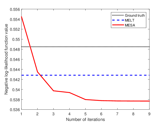
In this subsection, we test the numerical performance of MESA in convergence and optimality by computing the negative log-likelihood function value at each outer MM iteration. To compare with MELT [59], we consider the ULA in (53). As in [59], the frequency domain $[-\frac{1}{2},\frac{1}{2})$ is approximated by a set of $2N-1$ uniform gridding points and the true frequencies are selected from the gridding points to achieve the best performance for MELT, which though is not required in MESA. We also compare with the function value computed with the true values of parameters and denoted by “ground truth”. While the globally optimal function value is hard to obtain, it is expected that good accuracy is achieved if the obtained function value is smaller than the “ground truth”. The true noise power $\sigma^{o}$ is also fed into MELT as in [59].

In Experiment 1, $K=3$ sources are generated with DOAs such that the frequencies are taken as the 5th, 7th and 18th gridding points of MELT. We set $\text{SNR}=10\text{dB}$ and the number of snapshots $L=100$. The curve of the function value with respect to the index of the MM iteration of MESA is plotted in Fig. 1. It is seen that the function value decreases monotonically and converges in 9 iterations. MESA produces a function value smaller than the ground truth and MELT, indicated by the two horizontal dashed lines. MESA takes 534 inner iterations in total.

We tried a total number of 500 Monte Carlo runs and MESA always converges and produces a function value smaller than the ground truth. It performs better than MELT in 498 out of 500 runs.

In this subsection, we use the MRA in (54) and test the statistical efficiency of MESA for uncorrelated sources. RAM and MNOMP are considered only in the case of $K<M$.

In Experiment 2, We consider $K=7$ sources with DOAs satisfying that the frequencies are taken in $\left\{-0.43,-0.28,-0.21,-0.05,0.1,0.26,0.42\right\}$. We fix the number of snapshots $L=200$ and vary the SNR from $-10$ to $20$ dB. Our simulation results are presented in Fig. 2. It is seen that WLS and and MESA attain the CRB as $\text{SNR}\geq-5\text{dB}$, while SS-MUSIC always produces an error greater than the CRB. It is interesting to note that the results of MESA-1 and MESA are almost indistinguishable. In this case, the sample covariance is a good estimate of the data covariance and a single outer loop of MESA suffices to produce an accurate estimate.

In Experiment 3, we fix $\text{SNR}=10\text{dB}$, $L=100$ and vary $K$ from 2 to $N-1=13$. The $K$ sources are generated with $f_{k}=-0.44+0.98(k-1)/K$, $k=1,\dots,K$. Our simulation results are presented in Fig. 3. Again, WLS and MESA (and MESA-1) attain the CRB or even better whenever the number of sources is smaller or greater than the number of sensors, while SS-MUSIC cannot. NMOMP and RAM can accurately localize only a small number of sources, as expected.

In Experiment 4, we consider $K=3$ sources with frequencies given by $\left\{-0.2,0.1,0.1+\delta\right\}$ and vary $\delta\in\left\{0.001,0.003,\dots,0.029\right\}$. We fix the number of snapshots $L=100$ and $\text{SNR}=10\text{dB}$. It is seen in Fig. 4 that MESA attains the CRB for very closely located sources and thus has a higher resolution than the other methods. MNOMP fails to resolve the closely located sources. A gap is shown between MESA and MESA-1, implying that the MM iterations of MESA are useful to improve the resolution.

In Experiment 5, we consider $K=3$ sources with frequencies in $\left\{-0.2,-0.1,0.2\right\}$, where the first two sources are coherent with the correlation coefficient $e^{i\pi/3}$ (that can be changed to any other value on the unit circle). We use the nested array in (55) for DOA estimation to make sure that the assumptions of Theorem 1 are satisfied, which can be verified according to Proposition 1 since the source matrix $\bm{S}$ has rank 2 and $\text{Spark}\left(\Omega\right)\geq 6$ by noting that the nested array contains a 5-element ULA. We fix $L=100$ and vary the SNR from $-10$ to $20$dB. Our numerical results are presented in Fig. 5. It is seen that MESA has stable performance when the SNR is above 0dB, which is consistent with Theorem 1. Remarkably, MESA attains the CRB as in the case of uncorrelated sources. In contrast to this, SS-MUSIC and WLS do not have the same robustness as MESA. Satisfactory performance is also obtained by MNOMP and RAM. In this case, MESA performs better than MESA-1 since the solution to $\bm{R}_{\Omega}$ is significantly different from the sample covariance and an accurate initialization is unavailable.

We present in Fig. 6 results of one Monte Carlo run of the previous experiment (at $\text{SNR}=20\text{dB}$). It is seen that MESA can accurately estimate the frequencies/DOAs and the source power, validating Theorem 1. Interestingly, SS-MUSIC and WLS can accurately localize the two coherent sources but mislocate the third source that is uncorrelated with the other two. The reason underlies this behavior needs further investigation.

In Experiment 6, we repeat Experiment 5 by changing the nested array to the MRA in (54). In this case, it is difficult to verify the assumptions of Theorem 1. We present our results in Fig. 7. It is seen that all algorithms are affected to a larger extent by the source correlation as compared to the nested array case presented in Fig. 5. Differently from SS-MUSIC and WLS, MESA remains to be robust to source correlations. MNOMP has a poor performance in this case with a small array size.

In Experiment 7, we repeat Experiment 2 by fixing $\text{SNR}=10\text{dB}$ and letting the first and the fourth sources to be correlated with a correlation coefficient $\rho e^{i\pi/4}$, where the modulus $\rho$ changes from 0 (uncorrelated) to 1 (coherent). MNOMP and RAM are not usable since more sources than sensors are present. It is seen in Fig. 8 that the performance of all methods becomes worse as the correlation increases. In contrast to a steady performance loss of MESA, a sharp loss is shown for SS-MUSIC and WLS in the regime of highly correlated sources. As $\rho=1$, in fact, SS-MUSIC and WLS mislocate at least one of the sources in over $10\%$ of the Monte Carlo runs, while MESA always accurately localize the sources.

To sum up, we have shown by numerical results that MESA can statistically efficiently localize more uncorrelated sources than sensors and has robust performance in the presence of correlated and coherent sources. This makes it unique among existing coarray-based methods tailored for uncorrelated sources and sparse methods usable for a small number of sources. MESA-1 is a good accelerated approximation of MESA in general, while the latter has improved resolution and robustness. More simulation results can be found in our conference papers [1, 2].

To show (33), it suffices to show that

by identifying that $\check{\bm{Z}}=\widehat{\bm{Y}}-\bm{Z}$ and $\beta=\mu^{-1}$. To this end, observe that

where the equality is achieved if $\check{\bm{Z}}$ has the sign of $\bm{L}$. Since the last expression is minimized if $\|\check{\bm{Z}}\|_{\mathrm{F}}=(\|{\bm{L}}\|_{\mathrm{F}}-\beta)_{+}$, the overall function $g(\check{\bm{Z}})$ is therefore minimized at

completing the proof.

We first show the following lemma.

References

- [1] Z. Yang and X. Chen, “Maximum likelihood direction-of-arrival estimation via rank-constrained ADMM,” in CIE IEEE International Conference on Radar, available at https://1drv.ms/b/s!AnS77yS_s0jDh71z8Oh0Sz2fAdtNVw?e=1tYwvm, 2021.
- [2] X. Chen and Z. Yang, “Localizing more sources than sensors in presence of coherent sources,” in IEEE International Conference on Acoustics, Speech and Signal Processing (ICASSP), to appear, available at https://1drv.ms/b/s!AnS77yS_s0jDh71y0i_oUXFyVl085g?e=Jhxyom, 2022.
- [3] P. Stoica and R. L. Moses, Spectral analysis of signals. Upper Saddle River, NJ, US: Pearson/Prentice Hall, 2005.
- [4] Y. Barbotin, A. Hormati, S. Rangan, and M. Vetterli, “Estimation of sparse MIMO channels with common support,” IEEE Transactions on Communications, vol. 60, no. 12, pp. 3705–3716, 2012.
- [5] J. Li and P. Stoica, “MIMO radar with colocated antennas,” IEEE Signal Processing Magazine, vol. 24, no. 5, pp. 106–114, 2007.
- [6] W. Heylen and P. Sas, Modal analysis theory and testing. Katholieke Universteit Leuven, 2006.
- [7] M. J. Rust, M. Bates, and X. Zhuang, “Sub-diffraction-limit imaging by stochastic optical reconstruction microscopy (STORM),” Nature Methods, vol. 3, no. 10, pp. 793–796, 2006.
- [8] Y. Wang, J. Li, and P. Stoica, “Spectral analysis of signals: the missing data case,” Synthesis Lectures on Signal Processing Series, vol. 1, no. 1, pp. 1–102, 2006.
- [9] E. J. Candès, J. Romberg, and T. Tao, “Robust uncertainty principles: Exact signal reconstruction from highly incomplete frequency information,” IEEE Transactions on Information Theory, vol. 52, no. 2, pp. 489–509, 2006.
- [10] G. Tang, B. N. Bhaskar, P. Shah, and B. Recht, “Compressed sensing off the grid,” IEEE Transactions on Information Theory, vol. 59, no. 11, pp. 7465–7490, 2013.
- [11] A. Moffet, “Minimum-redundancy linear arrays,” IEEE Transactions on Antennas and Propagation, vol. 16, no. 2, pp. 172–175, 1968.
- [12] P. Pal and P. Vaidyanathan, “Nested arrays: A novel approach to array processing with enhanced degrees of freedom,” IEEE Transactions on Signal Processing, vol. 58, no. 8, pp. 4167–4181, 2010.
- [13] C.-L. Liu and P. Vaidyanathan, “Super nested arrays: Linear sparse arrays with reduced mutual coupling–Part I: Fundamentals,” IEEE Transactions on Signal Processing, vol. 64, no. 15, pp. 3997–4012, 2016.
- [14] J. Shi, G. Hu, X. Zhang, and H. Zhou, “Generalized nested array: Optimization for degrees of freedom and mutual coupling,” IEEE Communications Letters, vol. 22, no. 6, pp. 1208–1211, 2018.
- [15] P. P. Vaidyanathan and P. Pal, “Sparse sensing with co-prime samplers and arrays,” IEEE Transactions on Signal Processing, vol. 59, no. 2, pp. 573–586, 2011.
- [16] S. Qin, Y. D. Zhang, and M. G. Amin, “Generalized coprime array configurations for direction-of-arrival estimation,” IEEE Transactions on Signal Processing, vol. 63, no. 6, pp. 1377–1390, 2015.
- [17] T.-J. Shan, M. Wax, and T. Kailath, “On spatial smoothing for direction-of-arrival estimation of coherent signals,” IEEE Transactions on Acoustics, Speech, and Signal Processing, vol. 33, no. 4, pp. 806–811, 1985.
- [18] S. U. Pillai and B. H. Kwon, “Performance analysis of MUSIC-type high resolution estimators for direction finding in correlated and coherent scenes,” IEEE Transactions on Acoustics, Speech, and Signal Processing, vol. 37, no. 8, pp. 1176–1189, 1989.
- [19] K.-C. Tan and G.-L. Oh, “Estimating directions-of-arrival of coherent signals in unknown correlated noise via spatial smoothing,” IEEE Transactions on Signal Processing, vol. 45, no. 4, pp. 1087–1091, 1997.
- [20] F. Liu, J. Wang, C. Sun, and R. Du, “Spatial differencing method for DOA estimation under the coexistence of both uncorrelated and coherent signals,” IEEE Transactions on Antennas and Propagation, vol. 60, no. 4, pp. 2052–2062, 2012.
- [21] H. Tao, J. Xin, J. Wang, N. Zheng, and A. Sano, “Two-dimensional direction estimation for a mixture of noncoherent and coherent signals,” IEEE Transactions on Signal Processing, vol. 63, no. 2, pp. 318–333, 2014.
- [22] S. Qin, Y. D. Zhang, and M. G. Amin, “DOA estimation of mixed coherent and uncorrelated targets exploiting coprime MIMO radar,” Digital Signal Processing, vol. 61, pp. 26–34, 2017.
- [23] M. Wang and A. Nehorai, “Coarrays, MUSIC, and the Cramér–Rao bound,” IEEE Transactions on Signal Processing, vol. 65, no. 4, pp. 933–946, 2016.
- [24] C.-L. Liu and P. Vaidyanathan, “Cramér–Rao bounds for coprime and other sparse arrays, which find more sources than sensors,” Digital Signal Processing, vol. 61, pp. 43–61, 2017.
- [25] Y. Sun, P. Babu, and D. P. Palomar, “Majorization-minimization algorithms in signal processing, communications, and machine learning,” IEEE Transactions on Signal Processing, vol. 65, no. 3, pp. 794–816, 2016.
- [26] S. Boyd, N. Parikh, E. Chu, B. Peleato, and J. Eckstein, “Distributed optimization and statistical learning via the alternating direction method of multipliers,” Foundations and Trends® in Machine Learning, vol. 3, no. 1, pp. 1–122, 2011.
- [27] S. Diamond, R. Takapoui, and S. Boyd, “A general system for heuristic minimization of convex functions over non-convex sets,” Optimization Methods and Software, vol. 33, no. 1, pp. 165–193, 2018.
- [28] P. Stoica and A. Nehorai, “Performance study of conditional and unconditional direction-of-arrival estimation,” IEEE Transactions on Acoustics, Speech and Signal Processing, vol. 38, no. 10, pp. 1783–1795, 1990.
- [29] P. Stoica, E. G. Larsson, and A. B. Gershman, “The stochastic CRB for array processing: A textbook derivation,” IEEE Signal Processing Letters, vol. 8, no. 5, pp. 148–150, 2001.
- [30] M. Feder and E. Weinstein, “Parameter estimation of superimposed signals using the EM algorithm,” IEEE Transactions on Acoustics, Speech and Signal Processing, vol. 36, no. 4, pp. 477–489, 1988.
- [31] D. Starer and A. Nehorai, “Newton algorithms for conditional and unconditional maximum likelihood estimation of the parameters of exponential signals in noise,” IEEE Transactions on Signal Processing, vol. 40, no. 6, pp. 1528–1534, 1992.
- [32] R. O. Schmidt, “Multiple emitter location and signal parameter estimation,” IEEE Transactions on Antennas and Propagation, vol. 34, no. 3, pp. 276–280, 1986.
- [33] P. Stoica and K. C. Sharman, “Maximum likelihood methods for direction-of-arrival estimation,” IEEE Transactions on Acoustics, Speech, and Signal Processing, vol. 38, no. 7, pp. 1132–1143, 1990.
- [34] M. Viberg, B. Ottersten, and T. Kailath, “Detection and estimation in sensor arrays using weighted subspace fitting,” IEEE transactions on Signal Processing, vol. 39, no. 11, pp. 2436–2449, 1991.
- [35] B. Ottersten, M. Viberg, P. Stoica, and A. Nehorai, “Exact and large sample maximum likelihood techniques for parameter estimation and detection in array processing,” in Radar Array Processing. Springer, 1993, pp. 99–151.
- [36] H. Krim and M. Viberg, “Two decades of array signal processing research: The parametric approach,” IEEE Signal Processing Magazine, vol. 13, no. 4, pp. 67–94, 1996.
- [37] I. F. Gorodnitsky and B. D. Rao, “Sparse signal reconstruction from limited data using FOCUSS: A re-weighted minimum norm algorithm,” IEEE Transactions on Signal Processing, vol. 45, no. 3, pp. 600–616, 1997.
- [38] D. Malioutov, M. Cetin, and A. S. Willsky, “A sparse signal reconstruction perspective for source localization with sensor arrays,” IEEE Transactions on Signal Processing, vol. 53, no. 8, pp. 3010–3022, 2005.
- [39] E. Candès, J. Romberg, and T. Tao, “Stable signal recovery from incomplete and inaccurate measurements,” Communications on Pure and Applied Mathematics, vol. 59, no. 8, pp. 1207–1223, 2006.
- [40] J. Fang, J. Li, Y. Shen, H. Li, and S. Li, “Super-resolution compressed sensing: An iterative reweighted algorithm for joint parameter learning and sparse signal recovery,” IEEE Signal Processing Letters, vol. 21, no. 6, pp. 761–765, 2014.
- [41] Z. Yang and L. Xie, “Exact joint sparse frequency recovery via optimization methods,” IEEE Transactions on Signal Processing, vol. 64, no. 19, pp. 5145–5157, 2016.
- [42] C. Fernandez-Granda, “Super-resolution of point sources via convex programming,” Information and Inference: A Journal of the IMA, vol. 5, no. 3, pp. 251–303, 2016.
- [43] Z. Yang and L. Xie, “Enhancing sparsity and resolution via reweighted atomic norm minimization,” IEEE Transactions on Signal Processing, vol. 64, no. 4, pp. 995–1006, 2016.
- [44] J. Zhu, L. Han, R. S. Blum, and Z. Xu, “Multi-snapshot Newtonized orthogonal matching pursuit for line spectrum estimation with multiple measurement vectors,” Signal Processing, vol. 165, pp. 175–185, 2019.
- [45] Z. Yang, J. Li, P. Stoica, and L. Xie, “Sparse methods for direction-of-arrival estimation,” Academic Press Library in Signal Processing Volume 7 (R. Chellappa and S. Theodoridis, Eds.), pp. 509–581, 2018.
- [46] P. Pal and P. P. Vaidyanathan, “Coprime sampling and the MUSIC algorithm,” in 2011 Digital Signal Processing and Signal Processing Education Meeting (DSP/SPE). IEEE, 2011, pp. 289–294.
- [47] C.-L. Liu and P. Vaidyanathan, “Remarks on the spatial smoothing step in coarray MUSIC,” IEEE Signal Processing Letters, vol. 22, no. 9, pp. 1438–1442, 2015.
- [48] Y. D. Zhang, M. G. Amin, and B. Himed, “Sparsity-based DOA estimation using co-prime arrays,” in 2013 IEEE International Conference on Acoustics, Speech and Signal Processing. IEEE, 2013, pp. 3967–3971.
- [49] Z. Tan, Y. C. Eldar, and A. Nehorai, “Direction of arrival estimation using co-prime arrays: A super resolution viewpoint,” IEEE Transactions on Signal Processing, vol. 62, no. 21, pp. 5565–5576, 2014.
- [50] Q. Shen, W. Liu, W. Cui, and S. Wu, “Underdetermined DOA estimation under the compressive sensing framework: A review,” IEEE Access, vol. 4, pp. 8865–8878, 2016.
- [51] C. Zhou, Y. Gu, X. Fan, Z. Shi, G. Mao, and Y. D. Zhang, “Direction-of-arrival estimation for coprime array via virtual array interpolation,” IEEE Transactions on Signal Processing, vol. 66, no. 22, pp. 5956–5971, 2018.
- [52] S. Sedighi, B. S. M. R. Rao, and B. Ottersten, “An asymptotically efficient weighted least squares estimator for co-array-based DoA estimation,” IEEE Transactions on Signal Processing, vol. 68, pp. 589–604, 2019.
- [53] X. Xu, Z. Ye, Y. Zhang, and C. Chang, “A deflation approach to direction of arrival estimation for symmetric uniform linear array,” IEEE Antennas and Wireless Propagation Letters, vol. 5, pp. 486–489, 2006.
- [54] J. P. Burg, D. G. Luenberger, and D. L. Wenger, “Estimation of structured covariance matrices,” Proceedings of the IEEE, vol. 70, no. 9, pp. 963–974, 1982.
- [55] Y. I. Abramovich, D. A. Gray, A. Y. Gorokhov, and N. K. Spencer, “Positive-definite Toeplitz completion in DOA estimation for nonuniform linear antenna arrays. I. Fully augmentable arrays,” IEEE Transactions on Signal Processing, vol. 46, no. 9, pp. 2458–2471, 1998.
- [56] H. Li, P. Stoica, and J. Li, “Computationally efficient maximum likelihood estimation of structured covariance matrices,” IEEE Transactions on Signal Processing, vol. 47, no. 5, pp. 1314–1323, 1999.
- [57] D. Romero, D. D. Ariananda, Z. Tian, and G. Leus, “Compressive covariance sensing: Structure-based compressive sensing beyond sparsity,” IEEE Signal Processing Magazine, vol. 33, no. 1, pp. 78–93, 2015.
- [58] B. Kang, V. Monga, and M. Rangaswamy, “Computationally efficient toeplitz approximation of structured covariance under a rank constraint,” IEEE Transactions on Aerospace and Electronic Systems, vol. 51, no. 1, pp. 775–785, 2015.
- [59] P. Babu, “MELT—maximum-likelihood estimation of low-rank Toeplitz covariance matrix,” IEEE Signal Processing Letters, vol. 23, no. 11, pp. 1587–1591, 2016.
- [60] D. P. Wipf and B. D. Rao, “An empirical Bayesian strategy for solving the simultaneous sparse approximation problem,” IEEE Transactions on Signal Processing, vol. 55, no. 7, pp. 3704–3716, 2007.
- [61] Z.-M. Liu, Z.-T. Huang, and Y.-Y. Zhou, “An efficient maximum likelihood method for direction-of-arrival estimation via sparse Bayesian learning,” IEEE Transactions on Wireless Communications, vol. 11, no. 10, pp. 1–11, 2012.
- [62] A. Das and T. J. Sejnowski, “Narrowband and wideband off-grid direction-of-arrival estimation via sparse Bayesian learning,” IEEE Journal of Oceanic Engineering, vol. 43, no. 1, pp. 108–118, 2017.
- [63] B. Ottersten, P. Stoica, and R. Roy, “Covariance matching estimation techniques for array signal processing applications,” Digital Signal Processing, vol. 8, no. 3, pp. 185–210, 1998.
- [64] P. Stoica, P. Babu, and J. Li, “SPICE: A sparse covariance-based estimation method for array processing,” IEEE Transactions on Signal Processing, vol. 59, no. 2, pp. 629–638, 2011.
- [65] Z. Yang, L. Xie, and C. Zhang, “A discretization-free sparse and parametric approach for linear array signal processing,” IEEE Transactions on Signal Processing, vol. 62, no. 19, pp. 4959–4973, 2014.
- [66] H. Qiao and P. Pal, “Gridless line spectrum estimation and low-rank Toeplitz matrix compression using structured samplers: A regularization-free approach,” IEEE Transactions on Signal Processing, vol. 65, no. 9, pp. 2221–2236, 2017.
- [67] X. Wu, W.-P. Zhu, and J. Yan, “A Toeplitz covariance matrix reconstruction approach for direction-of-arrival estimation,” IEEE Transactions on Vehicular Technology, vol. 66, no. 9, pp. 8223–8237, 2017.
- [68] R. R. Pote and B. D. Rao, “Robustness of sparse Bayesian learning in correlated environments,” in IEEE International Conference on Acoustics, Speech and Signal Processing (ICASSP). IEEE, 2020, pp. 9100–9104.
- [69] M. Hong, Z.-Q. Luo, and M. Razaviyayn, “Convergence analysis of alternating direction method of multipliers for a family of nonconvex problems,” SIAM Journal on Optimization, vol. 26, no. 1, pp. 337–364, 2016.
- [70] F. Wang, W. Cao, and Z. Xu, “Convergence of multi-block Bregman ADMM for nonconvex composite problems,” Science China Information Sciences, vol. 61, no. 12, pp. 1–12, 2018.
- [71] Y. Wang, W. Yin, and J. Zeng, “Global convergence of ADMM in nonconvex nonsmooth optimization,” Journal of Scientific Computing, vol. 78, no. 1, pp. 29–63, 2019.
- [72] A. Barabell, “Improving the resolution performance of eigenstructure-based direction-finding algorithms,” in IEEE International Conference on Acoustics, Speech, and Signal Processing (ICASSP), vol. 8, 1983, pp. 336–339.
- [73] M. Fazel, H. Hindi, and S. P. Boyd, “Log-det heuristic for matrix rank minimization with applications to Hankel and Euclidean distance matrices,” in American Control Conference, vol. 3, 2003, pp. 2156–2162.
- [74] Z. Yang and L. Xie, “On gridless sparse methods for line spectral estimation from complete and incomplete data,” IEEE Transactions on Signal Processing, vol. 63, no. 12, pp. 3139–3153, 2015.
- [75] M. E. Davies and Y. C. Eldar, “Rank awareness in joint sparse recovery,” IEEE Transactions on Information Theory, vol. 58, no. 2, pp. 1135–1146, 2012.
- [76] B. Mamandipoor, D. Ramasamy, and U. Madhow, “Newtonized orthogonal matching pursuit: Frequency estimation over the continuum,” IEEE Transactions on Signal Processing, vol. 64, no. 19, pp. 5066–5081, 2016.