Tensor Perturbations and Thick Branes in Higher Dimensional Gauss-Bonnet Gravity
Abstract
A thick brane model with Gauss-Bonnet action in a homogeneous anisotropic spacetime is studied. By choosing a concrete metric ansatz, we show that this spacetime is stable against linear tensor perturbations under certain conditions. The graviton zero modes are also given. Besides, we examine a particular example in six-dimensional spacetime with a given warp factor. The coupled background scalar field and its potential are solved analytically. Furthermore, the effective potential of the Kaluza-Klein modes of the graviton is also discussed. We found that the effective potential can have singularities under certain conditions, which are related to the non-differentiability of the graviton zero modes.
I Introduction
General Relativity (GR) is the most successful gravitational theory which has been proposed for over one century. Though GR has been tested by many experiments, there are still a few unknown issues such as dark energy and dark matter that remain a mystery which indicates GR is not perfect yet. These issues strongly motivate us to consider the gravity theory beyond GR. During the past several decades, many schemes of modified gravity have been put forwardclifton_modified_2012. Among all the potential directions, the extra dimension scenario is attracted increasing attention. Historically, the very first extra-dimensional gravity model is the so-called Kaluza-Klein (KK) theory which aims to unify Einstein’s gravity and Maxwell’s electromagnetism by introducing an extra compact circle spacial dimension. The radius scale is small enough that it can not be detected. Moreover, extra dimensions are also preferred by the string theory.
On the other hand, the extra dimension could also be very large and spread infinitely. This possibility has been realized in the brane world model langlois_brane_2002; liu_introduction_2017. An outstanding advantage of the brane world scenario is that it could nicely solve the hierarchy problem arkani-hamed_hierarchy_1998; randall_large_1999; yang_gravity_2012; barbosa-cendejas_mass_2014; guo_localization_2013; hundi_fermion_2011. Nowadays, most of the related works on brane world model are carried out in five-dimensional spacetime. However, in five dimensions, the pure gravitational trapping mechanism of vector fields is still problematic and there is no remarkable proposal to solve the fermion mass hierarchy in the Standard Model yet. To overcome these mentioned issues, one may resort to higher dimensional brane world models. Particularly, brane solutions of a higher dimensional gravity with a real scalar field has been proposed recently cui_tensor_2020; zhong_tensor_2011; gu_full_2017; zhong_pure_2016; dzhunushaliev_thick_2020; PhysRevD.92.024011; cui_linear_2018; gu_stable_2018. Note that in the brane world model, one usually needs to solve higher derivative equations. One way to avoid this issue is to consider a specific higher-order polynomial combination of the Riemann tensor such that the field equation remains two derivatives. The resulted simplest option is the famous Gauss-Bonnet gravity. The Gauss-Bonnet term is particularly suitable for higher dimensional extension of GR because it is a purely topological term in four dimensions and does not contribute to the classical equation of motion. However, this term becomes dynamic in higher dimensions. Besides, such quadratic Gauss-Bonnet terms of curvatures also appears as a 1-loop correction of heterotic string theory GW86. Hence inspired by these works, in this paper, we pursue to investigate the Gauss-Bonnet brane world model. Related works of Gauss-Bonnet gravity in brane world model can be also seen in the literaturegiovannini_thick_2001.
Moreover, it is well known that the stability of thick branes is a very significant issue since brane systems should be stable at least under linear perturbations. This issue has been extensively investigated cui_tensor_2020; zhong_tensor_2011; giovannini_thick_2001; giovannini_gauge-invariant_2001; giovannini_curvature_2005; zhong_pure_2016; PhysRevD.92.024011; cui_linear_2018; gu_stable_2018. In addition, to match the gravitational experiments, the four-dimensional Newtonian potential should be recovered, which means that the zero modes of the graviton should be localized on the brane. Hence, we also devoted to studying the stability of tensor perturbations and the zero modes of the graviton of Gauss-Bonnet brane world model in this paper.
This paper is organized as follows: After introduction, we write down the D-dimensional Gauss-Bonnet action in the Section II, and then we give a particular anisotropic metric with two warp factors. The field equations under this metric ansatz are also given. In Section III, we mainly focus on the linear stability by computing the tensor perturbation equations. With these equations in hand, we solve the field equations analytically with a given scalar field and discuss the main property of the solution in Section IV. Some necessary technical details can be found in the Appendix A.
Through out the paper we adopt the following symbol conventions: We use the lowercase Latin letters running over to stand for the indices of the -dimensional spacetime. The lowercase Greek letters represent our four-dimensional Minkowski spacetime coordinates. Specially we use as the fifth extra spacial coordinate . The capital Latin live in the higher extra dimensional Euclidean space with . Moreover, through out the paper, we use the definition and the spacetime signature .
II Action, Field equation And Metric
Our discussion in this article is based on the following D-dimensional Einstein-Hilbert action with a Gauss-Bonnet term as
| (1) |
where , with the being the gravitional constant in D-dimensional spacetime, and is the Guass-Bonnet coupling constant which has dimension of . By using this action, we can directly derive the field equations by varing the action with respect to the metric tensor :
| (2) |
where is the energy-momentum tensor, and the lovelock tensor is coming from the contribution of the Gauss-Bonnet term clifton_modified_2012:
| (3) |
Parallel to the previous study such as in brane world model cui_tensor_2020. In this paper, we also consider a special anisotropic -dimensional bulk manifold , which is constructed by three subspaces:
- •
A 4-dimentional Minkowski spacetime ,
- •
An extra 1-dimensional noncompact space ,
- •
An extra d-dimensional Euclidean space .
Naturally, there should exist curved brane (like and brane) as well as flat brane. In this paper, we are particularly interested in a flat and static brane, of which the line element can be written as:
| (4) |
where and are two warped factors. The Gauss-Bonnet term in this metric can be computed directly as
| (5) | |||||
Some higher order terms will arise as grows larger till . Moreover, the field equations under this metric ansatz are:
| (6) |
| (7) |
| (8) |
where the prime ′ denotes the derivative with respect to the extra-dimensional coordinate . With a given matter distribution we can solve the equations above. But before we proceed, we should wonder whether this set of equations gives a reasonable solution, or under what condition they do so. To this aim, we need to first analyze the behavior under linear perturbation carefully.
III Linear Stability Under Tensor Perturbation
The perturbed equation can be very complicated for such a Gauss-Bonnet action(1) and bulk metric (4). The perturbed tensor equations of motion can be formally written as:
| (9) |
Usually, a linear perturbation can be decomposed into scalar, vector and tensor parts. Since these three perturbations are decoupled to each other. Hence here for simplicity, we just let alone the others and just focus on the tensor perturbation. Note that the tensor perturbation can impose various kinds of gauge conditions. Here we consider the most popular one which is the so-called the transverse-traceless(TT) gauge condition:
| (10) |
where obeys the TT gauge condition:
| (11) |
The tensor perturbation of brane-world model with TT gauge is carried out in cui_tensor_2020; zhong_tensor_2011. Similarly we compute the perturbed quantities step by step, from the perturbed Christoffel connection to the Riemann Curvature. The non-vanishing perturbed Christoffel connection are listed below:
| (12) |
By directly using the formula , one can computed all of the needed perturbation quantities which can be found in Appendix A. For example, the pertured Ricci tensor can be written as :
| (13) |
where are the d’Alembert and Laplace operator of Minkowski space and extra d-dimensional spacial Euclidean space respectively. Finally, after tedious but straightforward computation, we end up with components of the perturbed field equations:
| (14) |
We need to add that, the term of Eq.(III) has been eliminated with the consideration of the field equation(II). We will apply some mathematical methods to get some physical results from the equation above. First of all, we introduce a coordinate transformation to obtain a conformal-flat metric:
| (15) |
Then the perturbation equation (III) in such conformal flat coordinate reads:
| (16) |
This is a second-order linearized tensor equation that can be abstractly written as follows:
| (17) |
where are functions of coordinate defined by Eq.(III). Naturally, are we want to solve the equation, we are willing to decompose it into three different parts respectively:
| (18) |
We can firstly obtain the part, which is a Klein-Gordon equation:
| (19) |
and the Helmholtz equation for the extra d-dimentions:
| (20) |
What we left behind is a second-order ordinary differential equations for the extra fifth dimension:
| (21) |
We can always eliminate the one-order derivative term with one more factor , one can check that the Eq.(21) will be turned into a Shrodinger-like equationgu_full_2017:
| (22) |
where is the effective potential defined as
| (23) |
After that, we we can introduce a superpential and re-written the Hamiltonian of Eq.(22) into two operators and as what we do in supersymmetric quantum mechanics cooper_supersymmetry_1995:
| (24) |
With all this process, we can finally give the condition that makes sure the stability under linear perturbation. It immediately follows that we must have and in Eq.(19) and Eq.(20) for stability. And more importantly, we must have the graviton zero mode normalizable to avoid tachyon states.
Setting in Eq.(22), or , at least, we can obtain the ground state, or the graviton zero modes of this system:
| (25) |
With the help of these equations, we can set several restrictions for the perturbation. In the following, we will show the whole procedure through a specific example in the next section.
IV Brane Solution In 6d Spacetime
After perturbation analysis, we now turn to search for a particular brane solution. We choose as a non-trivial example. In 6-dimensions or the case , the line element reads
| (26) |
where is the coordinate of the sixth dimension which is compact.
Consider a background scalar field which is only the function of for a static flat brane, with the following action of the matter:
| (27) |
where is the self-interacting potential. Set in Eq. (II),(II),(II), the components of the field equations can be written as follows :
| (28) |
Moreover, the equation of motion for the background scalar field is:
| (29) |
In order to solve these equations, we give linearly combinations from Eq. (IV)
| (30) |
Then the main perturbation equation for this case reads:
| (31) |
We choose a particular smooth function for and which is also widely adopted in the literature liu_introduction_2017; gu_full_2017; yu_gravitational_2016; cui_tensor_2020; zhong_tensor_2011; guo_tensor_2016; yang_thick_2012; csaki_universal_2000; liu_domain_2011; zhong_pure_2016; PhysRevD.92.024011; cui_linear_2018 to solve and analyze the brane. Here we assume that
| (32) |
with , so that the metric(4) can be reduced to an at infinity. While the parameter was set to adjust the thickness of the brane. Substitute Eq.(32) into Eq.(IV), we will get the only one admissable equation as:
| (33) |
Note that it is easy to check that the ordinary differential equation :
| (34) |
has the solution:
| (35) |
where and are the first and second elliptic integrals respectively. Compare the above equation with the Eq. (33) we have
| (36) | |||||
| (37) |
Moreover, with the help of Eq.(29) to obtain the potential of the scalar field as:
| (38) |
Since the background scalar field should be real-valued, it proposes a restriction for the parameters in the ellipse integral, which means or :
| (39) |
The feasible region of the Gauss-Bonnet coupling constant is shown in Fig.1


To make things clear, we need to introduce the following dimensionless quantities:
| (40) |
Furthermore, the scalar field and its potential are shown in Fig.3 and Fig.3 respectively. The parameter is set to 1 in these two figures.
From Fig. 3, we should notice that the scalar field has two kinks for small and only one kink for large . So there must be a critical value of which will have one more kink once exceed.
This value can be found by solving the following equations:
| (41) |
Besides, it is remarkable that has the upper bound , which leads to a simpler and concise solution, and are displayed in Fig. 5 and Fig. 5:
| (42) | |||
| (43) |


Finally, we also want to explore the distribution of the energy density along the extra dimension , where . We introduce the dimensionless energy density:
| (44) |

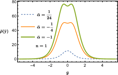
A lot of information can be obtained from the Eq.(44). First, we had better to stress that, the energy density is always positive definite under the condition (39). Second, the energy density behaves differently in various regions of the parameter space of and . Third, the peak of energy density will increase fastly when . Importantly, we notice that the energy density of the brane will be split into two different peaks as the value of decreases. This behavior is displayed in Fig. 7 and Fig. 7. The critical value of is determined by:
| (45) |
The split of the brane strongly implies that the brane may have some fine inner structure, which may have some physical results. It is worth stressing that, various kinds of reasons will result in a splitting brane, for example, a split brane caused by spacetime torsion is investigated in yang_thick_2012 and caused by a couple of multiple background scalar fields is study in bazeia_bloch_2004.
V Effective Potential
Now we going to discuss the effective potential. With the given warped factor (32), we are able to explore the effective potential (23). The results are depicted in Fig. 9 and Fig. 9. As a comparison, the effective potential of GR is drawn with a thin line in Fig. 9, we found that the well goes deeper as increases. By examining the second derivative with respect to , we found that the potential may split into two wells due to the Gauss-Bonnet correction term as shown in Fig. 9. In Fig. 9, a strange potential with two singularities is shown, compared to a normal smooth well. Note that although in the above section, we only discuss the brane with , the procedure can actually be carried out for general dimensions. Hence, the singularities in D-dimensions (D=4+1+d) are determined by the following equation:
| (46) |
So we can always find two symmetric singularities when .


The singularities of the potential should be accused of the non-differentiability of the graviton zero mode , from which we can see that they can still be normalized. The split effective potential is related to a graviton mode with two different peaks. These behaviors are shown in Fig. 10.

VI Conclusions
In summary, we investigate the Gauss-Bonnet thick-brane model in this paper. The behavior of this system under linear tensor perturbation with TT gauge is investigated in detail in this paper. The tensor perturbation equation can be reduced into the Klein-Gordon equation, Helmholz equation, and a second-order linear ordinary differential equation (Schrdinger-like equation). We conclude that the system is stable in tensor perturbation under certain conditions. Besides, the graviton zero mode is given.
Furthermore, with a coupling background scalar field and given warp factors, an analytical brane solution in six-dimensional spacetime was constructed. With which we can set a restriction for the Gauss-Bonnet coupling constant in the bulk action. The solution can be simplified a step further. In this case, we claim that the energy density will be split into two peaks with some particular parameter value. The critical value of the coupling constant is given to determine whether it will be split. At the end of the paper, we investigate the effective potential of the Schrdinger-like equation with respect to various parameters. The potential has a double-well at the bottom which is generated by the Gauss-Bonnet term, compared to one simple well of GR. Moreover, we found that the singularities of the potential should be accused of the non-differentiability of the graviton zero mode , and the split effective potential is related to a graviton mode with two different peaks.
Acknowledgements.
This work is supported by NSFC with Grants No.11775082.Appendix A Perturbational Quantities
What we want to obtain is the part of the perturbed field equation(9). We choose a method with brute force to evaluate. Theoretically, we can first find out the non-vanishing perturbed Christoffel connection, and then use it to construct the perturbed Riemann curvature tensor. But we do it inversely, we start from the needed quantities like the perturbed Ricci tensor, we might firstly decompose the contraction into:
| (47) |
It is the same for , but we need to expand it into more basic quantities firstly:
| (48) | |||||
And naturally, we may continue to expand the first four terms:
| (49) | |||||
| (50) |
| (51) |
| (52) | |||||
The three terms in (52) can be expanded as follow:
| (53) | |||||
| (55) | |||||
| (56) |
Some basic elements, like , appear repeatedly all the way, they can be decomposed into forms like . After expanding them into coordinate basis, all we need to do is comparing with the quantities given in (III).
| (57) | |||
| (58) | |||
| (59) | |||
| (60) | |||
| (61) | |||
| (62) |
Combining the quantities listed above to construct the perturbed Riemann curvature:
| (63) | |||
| (64) | |||
| (65) |
And with the same process:
| (66) | |||
| (67) | |||
| (68) | |||
| (69) | |||
| (70) | |||
| (71) |
We can get another set of perturbed Riemann Curvatue:
| (72) | |||
| (73) | |||
| (74) |
With all these elements given above, we can obtain all the necessary perturbed curvature.
In the end, we need to add that:
| (75) |
They can be evaluated in a similar way (see Appendix of Ref cui_tensor_2020). So the perturbed Ricci scalar vanished as . And for the perturbed Gauss-Bonnet term:
| (76) |
Since the first factor is proportional to and its derivative, the whole term will finally vanish because of the TT gauge condition (11).
For the perturbation of energy-momentum tensor , we only consider the perturbation caused by the fluctuation of the background metric csaki_universal_2000. That is to say:
| (77) |
or practically .
References
- [1] Timothy Clifton, Pedro G. Ferreira, Antonio Padilla, and Constantinos Skordis. Modified gravity and cosmology. Physics Reports, 513(1):1–189 (2012).
- [2] David Langlois. Brane cosmology. Progress of Theoretical Physics Supplement, 148:181–212, (2002).
- [3] Yu-Xiao Liu. Introduction to Extra Dimensions and Thick Braneworlds. arXiv: 1707.08541.
- [4] Nima Arkani-Hamed, Savas Dimopoulos, and Gia Dvali. The Hierarchy Problem and New Dimensions at a Millimeter. Physics Letters B, 429(3-4):263–272 (1998). arXiv: hep-ph/9803315.
- [5] Lisa Randall and Raman Sundrum. A Large Mass Hierarchy from a Small Extra Dimension. Physical Review Letters, 83(17):3370–3373 (1999). arXiv: hep-ph/9905221.
- [6] Ke Yang, Yu-Xiao Liu, Yuan Zhong, Xiao-Long Du, and Shao-Wen Wei. Gravity localization and mass hierarchy in scalar-tensor branes. Physical Review D, 86(12):127502 (2012). arXiv: 1212.2735.
- [7] Nandinii Barbosa-Cendejas, Alfredo Herrera-Aguilar, Konstantinos Kanakoglou, Ulises Nucamendi, and Israel Quiros. Mass hierarchy, mass gap and corrections to Newton’s law on thick branes with Poincare symmetry. General Relativity and Gravitation, 46(1):1631 (2014). arXiv: 0712.3098.
- [8] Heng Guo, Alfredo Herrera-Aguilar, Yu-Xiao Liu, Dagoberto Malagon-Morejon, and Refugio Rigel Mora-Luna. Localization of bulk matter fields, the hierarchy problem and corrections to Coulomb’s law on a pure de Sitter thick braneworld. Physical Review D, 87(9):095011 (2013). arXiv: 1103.2430.
- [9] R. S. Hundi and Soumitra SenGupta. Fermion mass hierarchy in a multiple warped braneworld model. J. Phys. G, 40:075002, (2013).
- [10] Zheng-Quan Cui, Zi-Chao Lin, Jun-Jie Wan, Yu-Xiao Liu, and Li Zhao. Tensor perturbations and thick branes in higher-dimensional f(R) gravity. Journal of High Energy Physics, 2020(12):130 (2020).
- [11] Yuan Zhong, Yu-Xiao Liu, and Ke Yang. Tensor perturbations of -branes. Physics Letters B, 699(5):398–402 (2011). arXiv: 1010.3478.
- [12] Bao-Min Gu, Yu-Peng Zhang, Hao Yu, and Yu-Xiao Liu. Full linear perturbations and localization of gravity on brane. The European Physical Journal C, 77(2):115 (2017). arXiv: 1606.07169
- [13] Yuan Zhong and Yu-Xiao Liu. Pure geometric thick -branes: stability and localization of gravity. The European Physical Journal C, 76(6):321 (2016). arXiv: 1507.00630.
- [14] Vladimir Dzhunushaliev, Vladimir Folomeev, Galia Nurtaeva, and Sergei D. Odintsov. Thick branes in higher-dimensional gravity. International Journal of Geometric Methods in Modern Physics, 17(03):2050036 (2020). arXiv: 1908.01312.
- [15] Bao-Min Gu, Bin Guo, Hao Yu, and Yu-Xiao Liu. Tensor perturbations of palatini branes. Phys. Rev. D, 92:024011 (2015).
- [16] Zheng-Quan Cui, Yu-Xiao Liu, Bao-Min Gu, and Li Zhao. Linear Stability of Thick Branes: Tensor Perturbations. Journal of High Energy Physics, 2018(11):83 (2018). arXiv: 1802.01454.
- [17] Bao-Min Gu, Yu-Xiao Liu, and Yuan Zhong. Stable Palatini braneworld. Physical Review D, 98(2):024027 (2018). arXiv: 1804.00271.
- [18] D. J. Gross and E. Witten. Superstring modifications of Einstein’s equations, Nucl. Phys. B 277, 1 (1986).
- [19] Massimo Giovannini. Thick branes and Gauss-Bonnet self-interactions. Physical Review D, 64(12):124004 (2001). arXiv: hep-th/0107233.
- [20] Massimo Giovannini. Gauge-invariant fluctuations of scalar branes. Physical Review D, 64(6):064023 (2001). arXiv: hep-th/0106041.
- [21] Massimo Giovannini. Curvature perturbations from dimensional decoupling. Classical and Quantum Gravity, 22(11):2201–2219 (2005). Publisher: IOP Publishing.
- [22] Fred Cooper, Avinash Khare, and Uday Sukhatme. Supersymmetry and Quantum Mechanics. Physics Reports, 251(5-6):267–385 (1995). arXiv: hep-th/9405029.
- [23] Hao Yu, Yuan Zhong, Bao-Min Gu, and Yu-Xiao Liu. Gravitational resonances on -brane. The European Physical Journal C, 76(4):195 (2016). arXiv: 1506.06458.
- [24] Wen-Di Guo, Qi-Ming Fu, Yu-Peng Zhang, and Yu-Xiao Liu. Tensor perturbations of -branes. Physical Review D, 93(4):044002 (2016). arXiv: 1511.07143.
- [25] Jie Yang, Yun-Liang Li, Yuan Zhong, and Yang Li. Thick Brane Split Caused by Spacetime Torsion. Physical Review D, 85(8):084033 (2012). arXiv: 1202.0129.
- [26] Csaba Csaki, Joshua Erlich, Timothy J. Hollowood, and Yuri Shirman. Universal Aspects of Gravity Localized on Thick Branes. Nuclear Physics B, 581(1-2):309–338 (2000). arXiv: hep-th/0001033.
- [27] Yu-Xiao Liu, Yuan Zhong, Zhen-Hua Zhao, and Hai-Tao Li. Domain wall brane in squared curvature gravity. Journal of High Energy Physics, 2011(6):135 (2011). arXiv: 1104.3188.
- [28] D. Bazeia and A. R. Gomes. Bloch Brane. Journal of High Energy Physics, 2004(05):012–012 (2004). arXiv: hep-th/0403141