Automated Algorithm Selection: from Feature-Based to Feature-Free Approaches

One of the most common approaches to ASP is to identify features using expert knowledge, and then train machine learning methods to predict the best performing algorithm(s) for an instance from its feature-profile (Kerschke et al. 2018a). However, identifying features that are significant in determining performance is complex, usually requires hand-crafting (Nudelman et al. 2004; Hutter et al. 2014; Smith-Miles and van Hemert 2011; Pihera and Musliu 2014), and often is not intuitive. Often the approach must also be combined with a feature-reduction method to simplify learning, e.g Principal Component Analysis (PCA) (Smith-Miles et al. 2014; López-Camacho et al. 2013), and understand the correlations between features and algorithm performance.

Cruz-Reyes et al. 2012 have used meta-learning and hyper-heuristics to solve ASP in the domain of 1D-BPP. Their methodology relies on data collected from past experience to characterise algorithm performance and it is divided into three phases: initial training, prediction, and training with feedback. The output of the training phase is a trained model that relates the problem characteristics to the algorithms’ performance — this model is used to predict the best algorithm for a new given instance in the prediction phase. The new solved instances are then incorporated into the knowledge base to improve the selection quality. They used five deterministic heuristics and two non-deterministic algorithms with 1D-BPP. Three machine learning methods are compared — Discriminant Analysis (DA) (Pérez et al. 2004), a decision tree to build the selectors and a Self-Organizing Map (SOM) (Haykin et al. 2009) to implement the selection system with feedback. Five features were used as input. Their method obtained 76% accuracy with DA and 81% accuracy with decision tree to select the best algorithm. Also, the accuracy increased from 78.8% with initial-training up to 100% when using SOM with feedback and the number of problem characteristics was the minimum.

López-Camacho et al. 2013 also studied ASP in the packing domain using a wide range of 23 features and six heuristics within an evolutionary hyper-heuristic framework. They studied the correlation between the structure of 1D- and 2D-BPP instances and the performance of the solvers using PCA (Ringnér 2008) as a knowledge discovery method. Most of the used features are related to 2D-BPP and a subset of nine features, including means and standard deviation (std) of the item sizes, are considered that is strongly correlated with the heuristics performance after the feature-reduction. They analysed the distribution of feature values across the PCA map and their analysis suggested that there are indeed correlations between instance characteristics and heuristic performance. Brownlee et al. 2018 have used ten BPP features that are related to the distribution of item sizes within each instance and performance features to analyse the relationship between the training data and automatic design of algorithms. They investigated the distributions of values for features over the instances in benchmark sets, and how these distributions relate to the performance of algorithms built by automatic design of algorithms. They concluded that high variation in some of these features, including mean, standard deviation and maximum of item size, is a strong indicator for good fitting to the training instances and to achieve good performance for automatic design of algorithms.

A different type of approach was proposed by Ross et al. 2002 that could be used for ASP with constructive approaches to solution generation; rather than deriving features from the original description of an instance, a small number of features were derived from the current instance state each time a heuristic was applied. A learning classifier system XCS (Wilson 1995) was used to map a set of problem-states to specific heuristics. An approach that tries to avoid having to hand-craft good features was described in (Sim et al. 2012) who evolve the parameters of a feature design method for 1D bin-packing problems to that best improve the performance of k-Nearest Neighbours (KNN) classifier (Shalev-Shwartz and Ben-David 2014).

Another ASP approach that does not explicitly rely on feature identification and extraction was proposed by Sim et al. 2015. Here, a system continuously generates novel heuristics which are maintained in an ensemble, and samples multiple problem instances from the environment. Heuristics that ”win” an instance (perform best) are maintained. This was shown to rapidly produce solutions and generalise over the problem space, but required a greedy method of actually selecting between generated heuristics and hence does not fit with the classical ASP definition.

Although feature-based approaches have been shown to work well in domains in which there is no sequential information associated with an instance description²² 2 although it could be argued that some sequential information is implicit in those approaches just mentioned that dynamically calculate problem state and use this to select heuristics (Sim et al. 2012; Ross et al. 2002)., domains in which data arrives in a continual stream are more challenging. Statistical approaches to defining features for streaming data are complex, and developing algorithm selectors to tackle streaming data poses considerable challenges due to potentially large streams, the fact that the order of data points cannot be influenced and that the underlying distribution of the data points in the stream can change over time. A recent survey article describing the state-of-the-art in algorithm-selection (Kerschke and Trautmann 2019) highlighted a pressing need to develop automated algorithm-selection methods that are capable of learning in the context of streaming data. A supervised-learning approach was used by van Rijn et al. 2018; van Rijn et al. 2014 to predict which classifier performs best on a (sub)stream. Unsupervised learning approaches such as stream-clustering have been used to identify, track and update clusters over time (Carnein et al. 2017; Gong et al. 2017). However, due to the huge space of parameter and algorithm combinations, clear guidelines on how to set and adjust them over time are lacking (Mansalis et al. 2018; Carnein and Trautmann 2019; Amini et al. 2014).

Recently, deep learning algorithms have gained some traction in the ASP field due their ability to learn from extremely large datasets in reasonable time. Mao et al. 2017 proposed a heuristic performance predictor using a deep neural network trained on a large set of instances of variable sized 1D bin-packing problem using 16 features as input, grouped into item, box and cross features. Their prediction system has achieved up to 72% validation accuracy to select the best performing heuristic that can generate a better quality bin-packing solution. To eliminate the arduous task of manually designing features, Loreggia et al. 2016 proposed a deep learning approach to automatically derive features in SAT and CSP domains assuming that any problem instance can be expressed as a text document. Unlike previous works e.g. (Smith-Miles et al. 2014; López-Camacho et al. 2013) that derive features from features automatically using PCA, their approach automatically derives features from a visual representation of the problem instances (i.e. converting the text files into grey-scale square images), which can be used to train a conventional neural network to predict the best solver for the instance. Although their approach obtained better results than the SBS, it was not able to outperform over the approaches that use regular manually crafted features. Although concerned with learning an optimisation method rather than algorithm-selection, Hu et al. 2017 used a deep reinforcement learning (a Pointer Network), with 3D-BPP to optimize the sequence of items to be packed into the bin by choosing the sequence, orientation and empty maximal space to pack cuboid shaped items. They claimed that their proposed method has obtained about 5% improvement over a well-designed heuristic.

As mentioned in the introduction, in a recent conference paper, Seiler et al. 2020 adopted and adapted the LSTM approach we proposed in (Alissa et al. 2019) to be applicable to the Euclidean TSP domain, also using an evolved (and balanced) dataset (1000 instances) with two TSP solvers. They compared a feature-based approach using four different classical ML classifiers to a feature-free approach using deep learning Convolutional Neural Networks (CNNs). Due to the large TSP-related feature sets, they conducted a data analysis and automatic feature selection to choose adequate set of 15 most relevant features. Their results show that the feature-based approach improved over the SBS performance but still quite far away from the performance of the oracle-like VBS. The feature-free approach matches the performance of the quite complex classical ML approaches, despite being solely based on raw visual representation of the TSP instances. Although TSP is not an online or sequential problem, the work of Seiler et al. 2020 borrows the key concept of our proposed method, i.e. that the raw data defining an instance can be used without modification as input to a selection algorithm.

The approach proposed in this paper differs substantially from the previous work just described in that it abandons the need to derive features from a dataset, circumventing the associated issues. In contrast to some previous research which extends Rice’s diagram to encapsulate a broader agenda relating to the relative power of algorithms (e.g. Smith-Miles et al. 2014), our proposed method shrinks Rice’s diagram through bypassing the feature extraction block. Furthermore, as far as we are aware, it provides the first example of applying a recurrent-neural network as an algorithm-selector to data which has sequential characteristics. Although such networks have demonstrated ground-breaking performance on a variety of tasks that include image captioning, language translation and handwriting recognition (Lipton et al. 2015), their applicability has not been exploited within the ASP domain.

We select a Recurrent Neural-Network (RNN) as a deep learning method designed to learn from sequence data. RNNs are one of the two most common architectures described under the umbrella term Deep Learning (DL). They differ from Feedforward Neural Networks due to the presence of cyclic connections from each layers’ output to the next layers input, with feedback loops returning to the previous layer (Fig 2-a) (Wang and Raj 2017; Lipton et al. 2015). This structure prevents traditional back-propagation being applied since there is not an end point where the back-propagation can stop. Instead, Back Propagation Through Time (BPTT) is applied: the RNN structure is unfolded to several neural networks with certain time steps and then the traditional back-propagation is applied to each one of them (Fig 2-b) (Wang and Raj 2017). RNNs are specifically designed to learn from sequence data where sequential information explicit in the order of sequences is used to identify relationships between the data and the expected outputs from the network.

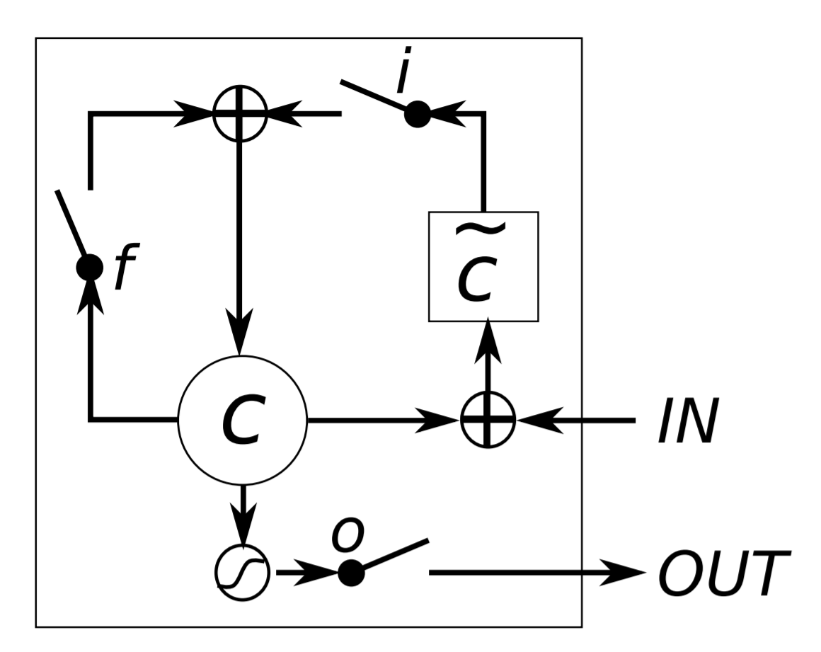
In this study we use a specialised RNNs known as a Long Short-Term Memory (LSTM) (Hochreiter and Schmidhuber 1997) and Gated Recurrent Unit (GRU) (Cho et al. 2014) that have been shown to be efficient and effective in learning long-term dependencies from sequences of ordered data. LSTM neural networks incorporate additional gates that can retain, retrieve and forget information (i.e. the network states) over long periods of time (Graves 2012). These gates are simply a combination of addition, multiplication and non-linear functions (Nielsen 2015). Three main gates are used in the LSTMs input, output and forget gates and three main states input, hidden and internal cell states. Basically, internal states are the ”memory” of the LSTM block, hidden states represent values that come from the previous time step, and the input state is the result of the linear combination between the hidden state and the input of current time step. In the LSTM network, the classic neurons in the hidden layer are replaced by memory blocks. Fig 3 shows that the LSTM’s input comes from the network through the input gate and the only outputs from the LSTM to the rest of the network emanate from the output gate multiplication. The input gate determines how much of the new memory content is added to the memory cell, the output gate modulates how much of the internal state would be exposed to the external network (higher layers and the next time step), while the forget gate defines how much of the existing memory is forgotten. GRU is a recent variation on LSTM with only two gates, update and reset gates which decide what information should be passed to the output. The update gate decides how much of the past information would be passed to the future while the reset gate determines how much to be forgotten. Also, GRU does not use the internal state and instead uses the hidden state to transfer information through the time steps (Chung et al. 2014). A more comprehensive description of the rapidly expanding field of DL, which has many competing, but no prevalent architectures, is outwith the scope of this study.

We evaluate six well-known classical machine learning techniques (Shalev-Shwartz and Ben-David 2014) from the literature: Neural Network (NN); Decision Trees (DT); Random Forest (RF); Naive Bayes (NB); k-Nearest Neighbours (KNN) and Support Vector Machine (SVM). Each is used in its standard form, parameterised using grid-search and bayesian optimisation as described in section 6. The success of ASP methods that rely on feature extraction depend critically upon the chosen features (Smith-Miles and Lopes 2012) and on the classification method used to learn the correlation between the features and best-performing heuristic.

The traditional method of dealing with ASP is to hand-design features and then extract them from the instance data. Here, we use a set of features collated from multiple papers in the literature where algorithm-selection methods have been applied to bin-packing (Cruz-Reyes et al. 2012; López-Camacho et al. 2013; Brownlee et al. 2018), discussed in section 2. The features are given below:

1. 1.

   Mean item size divided by bin capacity $C$ (Brownlee et al. 2018; López-Camacho et al. 2013; Cruz-Reyes et al. 2012; Mao et al. 2017);

2. 2.

   Standard Deviation (std) in the item sizes divided by bin capacity $C$ (Brownlee et al. 2018; López-Camacho et al. 2013; Cruz-Reyes et al. 2012; Mao et al. 2017);

3. 3.

   Maximum item size divided by bin capacity $C$ (Brownlee et al. 2018; Mao et al. 2017);

4. 4.

   Minimum item size divided by bin capacity $C$ (Brownlee et al. 2018; Mao et al. 2017);

5. 5.

   Median item size divided by bin capacity $C$ (Brownlee et al. 2018);

6. 6.

   Maximum item size divided by minimum item size (Brownlee et al. 2018);

7. 7.

   The ratio of small items of size $\omega$ $\leq$ $C/4$ (Ross et al. 2002);

8. 8.

   The ratio of medium items of size $C/4$ $\textless$ $\omega$ $\leq$ $C/3$ (Ross et al. 2002);

9. 9.

   The ratio of large items of size $C/3$ $\textless$ $\omega$ $\leq$ $C/2$ (Ross et al. 2002);

10. 10.

    The ratio of huge items of size $\omega$ $\textgreater$ $C/2$ (Ross et al. 2002).

It should be clear that these features do not provide any information about the sequential characteristics implicit in the data-stream that describes each instance (i.e. the order of items to be packed). Rather, they describe statistical properties relating to the distribution of the item sizes. The 10 features were extracted for each of 16,000 instances contained in DS(1-5) and used as input to the classical machine learning models.

As mentioned in section 6, 10-fold cross validation is used to train the models taking 10% of the training instances to verify each fold and to evaluate the generalisation error. Table 13 in the appendix shows results achieved on the validation sets used during training for the DL models (LSTM and GRU) and all 6 ML models. Table 2 shows the results achieved on each test set with the model obtained from training on the full training set. We report the classification accuracy as an indicator of the LSTM’s, GRU’s and ML’s predictive abilities. Using Wilcoxon signed-rank test, significance is calculated in a pairwise fashion and corrected for multiple comparisons with the Bonferroni method between the DL techniques and VBS, SBS and best of the ML techniques for each dataset, and between the best ML technique and the SBS. p-values are shown in table 14 in the appendix. Table 3 additionally shows the comparison between the LSTM, GRU, the best ML technique and the SBS over the different test sets.

Results obtained from deep learning LSTM and GRU approaches are significantly better than the results using classical ML techniques (i.e. $\mathcal{H}_{0}(1)$ is rejected). We observe that the DL results from the validation and test sets on DS2 and DS4 are better than on the other datasets suggesting that the sequential correlations are easier to find in the datasets comprised of item weights generated from a wider range of values following a uniform distribution. It might be that the instances that are evolved with items in the range [40-60] may have fewer distinct patterns (i.e. sequential information) than instances generated with items in the range [20-100], regardless of the length of the instances. It is well known that problems with an average weight of $\frac{C}{3}$ are more difficult to solve (Falkenauer and Delchambre 1992) and it is interesting that problems with those characteristics are more difficult to classify using LSTM or GRU, i.e. instances from DS(1,3) with item weights generated from a narrow range of values [40,60] which is an average of one third of bin capacity 150. Although all the ML results show relatively poor performance compared to the DL methods, it does comparatively better, in the most cases, on the two longer datasets DS3 and DS4 than the shorter ones DS1, DS2 on the validation set, while this is true only for the comparison between DS2 and DS4 on the test set. It might be that the longer instances result in more distinct values for the extracted features, hence increasing the ability of the ML techniques to classify correctly.

Although training the LSTM and GRU on the longer instances requires significantly more learning iterations before the models converge, it is interesting to note that for both distributions the results obtained by the LSTM and GRU on the longer instances (e.g. DS4) exceed those reported on the datasets with smaller numbers of items (e.g. DS2) on the validation set. We conjecture that the longer instances provide the DL models with more sequential information, hence increasing the ability to determine patterns in the item sequences. The ML results partially concur with the LSTM and GRU results in this respect, i.e. results on DS3 are more accurate than DS1 (apart from NB) and those for DS4 are more accurate than for DS2 on the validation set. For both DL and ML models, this is true only for the comparison between DS2 and DS4 on the test set. The results of the LSTM and GRU experiments conducted on the combined DS5 set show intermediate results with accuracy between that achieved on the experiments on instances with uniform distribution and those with Gaussian distribution. These models are able to generalise over instances sampled from all of the problem lengths and the different weight distributions investigated without any apparent loss of precision. In contrast, the ML experiments conducted on the combined DS5 sets show worse results than most of the other experiments. This demonstrates that the feature-based approach is weak in its ability to generalise over instances with different characteristics and highlights its reliance on the quality of the designed features, in contrast to the LSTM and GRU approaches.

Table 4 presents confusion matrices of the LSTM, GRU and best ML techniques extracted from the experiments conducted on the test set DS5, the rest of the confusion matrices are shown in table 15 in the appendix. In most cases, the DL models were most frequently confused when attempting to classify the sequences identified as being solved best by FF and BF. It is interesting to note that (Alissa et al. 2019) previously showed that these two algorithms are extremely close in terms of their two largest principal components in a space defined by a 4-d vector containing the performance metric of each of the 4 heuristics for each instance. Similarly, instances labelled as NF appear to be the easiest to identify and correspondingly are the most isolated in the performance-space. As noted previously in (Alissa et al. 2019), it appears that the patterns shown by conducting a PCA of the performance space are correlated with the ability of LSTM to identify the best performing algorithm from the raw instance sequences. On the other hand, the ML models are frequently confused between FF and BF (similarly to LSTM and GRU), but the ML models are also confused between FF and WF. In terms of the accuracy to classify NF, ML results partly concur with the DL results, in that NF instances are easier to classify only in DS1 and 3.

Purely out of our interest, we conducted a 10-fold cross validation on DS4 using only the item sizes information defining the original instances (i.e. without any features) directly supplying all item sizes at once to two of the classical ML techniques: the Multi Layer Perceptron (MLP) and the Random Forest (RF) classifiers. The ML techniques were used directly from Weka (Eibe et al. 2016) without altering any of the default parameters. The RF achieved 67.55% accuracy. MLP was equally successful, achieving 67.08% accuracy. Although better than expected, we found that a DL approach that has been designed to work with sequential data provides more informative results.

In terms of Falkenauer’s fitness, for all experiments the DL selectors significantly improve on both the SBS (BF for all datasets) and the classical ML techniques (i.e. $\mathcal{H}_{0}(1,2)$ are rejected), and are very close to the VBS. Also, the best ML techniques improve over the SBS significantly (i.e. $\mathcal{H}_{0}(3)$ is rejected), P-values are shown in table 14 in the appendix.

Figure 4 shows cumulative distribution plots over the test sets of 800 instances from each DS(1-5) in terms of Falkenauer’s fitness: the plots show the percentage of instances that are solved with an distance d_p of the oracle-like VBS (the perfect mapping) given the solver predicted by a model $m$. The distance $d$ is calculated as d_p= (VBS_{Falkenauer’sfitness} $-$ Selector_{Falkenauer’sfitness}). Hence, d_p $\geq$ 0 and d_p = 0 represents the optimal.

Results show that the RNN-LSTM/GRU solves between 80.88%-97.63% of the instances within 5% of the VBS performance, compared to 50%-62.2% using the SBS. This represents a 30.88% to 35.43% improvement on DS(1-5). The best ML technique solves 67.13%-78.63% instances with 5% performance difference in all the datasets which is 16.43%-17.13% improvement over the SBS. Using either LSTM or GRU, between 99.63% and 100% of the instances can be solved within 30% of VBS for DS(1-5): in contrast, using the best ML technique, this is only true on DS(1,3). From the figure, it is clear that the best ML technique can only solve 100% of instances if we consider a performance difference of 40% in DS(2,4,5). It is interesting to note that although the SBS solves a lower percentage of instances than both the DL and the best ML technique if we consider a difference of 5% of the VBS performance, it manages to solve all the instances at 20% of the VBS in all the datasets. Although the ML techniques improve over the SBS in the most cases, they are not as good as the LSTM/GRU and are not as close to the VBS as the DL methods.

It is noticeable from the evolved instances in (Alissa et al. 2019) that the performance of the heuristics is skewed towards FF and BF, i.e. these heuristics are either the best or second best choice for all instances. This means that even if the selector mis-classified most of the NF and WF instances by choosing FF or BF, it will still achieve high performance. Therefore, as well as comparing the two approaches based on the performance metric and classification accuracy, we additionally compare them in terms of the number of bins used to pack a set of items to get a clearer understanding of their relative performance.

The overall objective of the BPP is to minimise the number of bins used to pack a set of items. Ultimately, the number of containers defines the cost of any real-world solution. Table 5 shows the number of bins required to pack all 800 test instances for each DS(1-5) and contrasts this against the lowest possible number of bins used by the VBS and the number of bins needed using the algorithms predicted by LSTM, GRU and traditional ML selectors. The LSTM and GRU use between 1.32% and 2.39% fewer bins than the SBS and between 0.21% and 1.52% more than the VBS. On DS4, GRU uses over 1150 bins fewer than the SBS and only 176 (0.21%) more than the VBS which uses 83,823 bins. While the ML techniques use between 1.85% more bins and up to 0.92% fewer bins than the SBS and 1.87% to 4.74% more than the VBS.

After normalising the number of bins $b^{\prime}$ used by the predicted algorithm (described in section 6), a Wilcoxon signed-rank test is used to evaluate significance in a pairwise fashion for all comparisons of bins and corrected for multiple comparisons with the Bonferroni method. Table 14 in the appendices shows the p-values of $b^{\prime}$ in a pairwise fashion to the bins used by the SBS and the VBS. Based on these p-values, Table 6 shows the comparison between the LSTM, GRU the best ML technique and the SBS over the different test sets in terms of bins. For all experiments the DL selectors significantly improve on both the SBS (BF for all datasets) and the classical ML techniques (i.e. $\mathcal{H}_{0}(1,2)$ are rejected), and are very close to the VBS. While the best ML techniques improve over the SBS significantly (i.e. $\mathcal{H}_{0}(3)$ is rejected) only on DS(1,3).

Figure 5 shows the cumulative distribution plots over the test sets of 800 instances from each DS(1-5) in terms of number of bins, where the difference d_b=(Selector_usedbins $-$ VBS_usedbins) $\geq$ 0 and d_b=0 is the best. In terms of the percentage of instances that are solved by each method, LSTM/GRU solves 82.13%-98.75% within 5% VBS while the best ML technique solves 69.5%-84.63% and 53%-89% by SBS for DS(1-5). For higher values of differences from the VBS, the results depend on the dataset used. On DS(1,3), 99.13%-100% of the instances are solved by LSTM/GRU compared to 93.25%-93.38% solved by ML within 10% of VBS and both techniques solve all the instances within 20% VBS. On DS(2,4,5), 99.88%-100% instances solved by LSTM/GRU while 98.13%-100% by best ML technique within 30% VBS. The SBS manages to solve 99.6% to all instances within 10% VBS on DS(1,3) and within 20% VBS on DS(2,4,5).

In summary, the results presented indicate that a deep learning method is clearly superior to using a classical prediction method trained with extracted features. Furthermore, as shown in the last column in Tables 3 and 6, we infer that the choice of deep method itself has minimal significant effect, i.e. it is the switch to a learning method that captures sequential information that provides the gain in performance.

Based on the analysis above, we consider only BF and FF as potential heuristic solvers. We generate using datasets with that are increasingly discriminatory with respect to these heuristics, using the magnitude of the performance gap between the two heuristics applied to the same instance as a proxy for quantifying implicit structure within the instance that is exploited by one heuristic or the other. Specifically, we generate instances at random from a given distribution, measure the Falkenauer fitness $BF_{i}$, $FF_{i}$ on each, then discard instances where $|BF_{i}-FF_{i}|<\tau$, for $0\leq\tau\leq 0.06$. Thus, higher values of $\tau$ should lead to more structured instances. 1750 instances are generated in this manner from the distributions in table 1 corresponding to DS1 and DS2. In each data set, we accumulate 1000 instances best solved by BF and 750 best solved by FF, to reflect the performance distribution as described in the next section.

From each dataset of 1750 instances, we create a balanced dataset for training but evaluate performance on a test-set whose composition is reflective of the distribution of instances. The training set thus contains 500 instances best solved by each BF and FF, while the test set includes 750 instances, 500 instances best solved by BF and 250 for FF to reflect the imbalance performance distribution. Similarly to the previous experiments, 10-fold cross validation is used to train the GRU, NN and RF models taking 10% of the training instances to verify each fold and to evaluate the generalisation error. Table 16 in the appendix shows results achieved on the validation sets used during training for the GRU, NN and RF models on RDS_τ(1,2). Table 8 shows the results achieved on each threshold test set with the models obtained from training on the full training set. We report the classification accuracy as an indicator of the GRU’s, NN’s and RF’s predictive abilities. For RDS_τ1, where item-sizes are drawn from a Gaussian distribution, we do not observe any obvious trend as the ‘structure’ in the instances increases for both the feature-free and features-based approaches. As mentioned in Section 7.1, the instances generated using this range of values [40, 60] and Gaussian distribution are more difficult to classify even with the evolved instances (i.e. they have maximum ‘structure’ threshold). In contrast, in RDS_τ2 where the item-sizes are drawn from a uniform-random distribution, there is a general trend of feature-free approach performance increasing as $\tau$ increases, with high-level of classification accuracy ($>$75%) exhibited when $\tau\geq 0.05$. While this trend is much less obvious with the feature-based approaches with classification accuracy at its best is 67.87%.

Table 9 shows the number of bins required to pack all 750 test instances for each RDS_τ(1,2) per threshold and contrasts this against the number of bins used by the SBS and the number of bins needed using the algorithms predicted by each of GRU, NN and RF selectors. In general, the feature-free approach wastes less and saves more bins than the feature-based approaches. On RDS_τ1, the GRU uses between 0.18% and 0.72% more bins than the SBS, while NN uses between 0.14% and 1.00%; RF uses 0.20% and 0.76% more bins than the SBS. Although both approaches fail to save bins with thresholds less than 0.04 on RDS_τ2, the GRU uses 0.33% and 0.43% fewer bins than the SBS for thresholds 0.06 and 0.05 respectively, NN fails to save any bin and RF saves only 0.04% using 0.05 threshold. On RDS_τ2 with threshold 0.05, GRU uses 170 bins fewer than the SBS while RF saves only 16 bins. Using Wilcoxon signed-rank test, significance is calculated in a pairwise fashion and corrected for multiple comparisons with the Bonferroni method between the GRU, ML techniques and SBS for each threshold of dataset RDS_τ(1,2). p-values are shown in table 17 in the appendix. Table 10 additionally shows the comparison between the GRU, ML techniques and the SBS over the different thresholds test sets.

As widely recognised in the literature, developing an understanding of the region(s) of an instance-space in which an algorithm performs well Smith-Miles et al. 2010 is essential for performing algorithm-selection. This enables training datasets to be collected that include representative instances from the regions of strength of each algorithm considered. The task for the algorithm-selection designer is then to find a mapping between instances and algorithms: either by extracting informative features from the dataset (’feature-based’) or using the raw-instance data as input (’feature-free’).

In figure 6 we demonstrated that two of the best performing heuristics for bin-packing (FF and BF) perform very similarly on a large set randomly generated instances, i.e. the instances are not discriminatory with respect to the heuristics we consider: this is line with results that have previously been reported in multiple domains (Cho et al. 2008; Smith-Miles and van Hemert 2011) concerning randomly generated benchmarks. This motivated our decision to evolve instances that specifically maximised the performance-gap between heuristics (figure 6(b)). We hypothesised that the evolved instances contain some implicit structure that is exploited by a particular heuristic that enables it to perform well. Furthermore, we suggested that increasing levels of discrimination between algorithms on an instance corresponds to increasing levels of ‘structure’ within the instance-data. We therefore created fourteen further datasets in which control the level of structure in randomly generated instance using the performance-gap between two heuristics as a proxy for structure. We then evaluated the performance of both feature-free and feature-based approaches on these datasets.

A systematic analysis showed that in the case of instances generated at uniform-random, increasing the structure dramatically improved the performance of the GRU model in terms of classification accuracy while this is less obvious using the feature-based NN and RF models. However, there is no discernible trend from instances generated from a Gaussian distribution. One explanation for this is that the combined effect of drawing from a Gaussian distribution and restricting the item-sizes to a narrow range (40-60 in this case) results in instances which are very similar, i.e. in which it is difficult to find unique structure. The number of ties observed between BF and FF on this dataset (see table 7 lends some weight to this). Alternatively, a different method of creating structure could be considered, for example, in relation to one or more features of the datasets described in section 5.3.

The results reported in section 7 on DS1-4 and in table 8 suggest that the proposed GRU model that uses only the sequence of item-sizes as input performs well on datasets in which some structure exists within the data ($\tau\geq 0.05$). Given that is well-known that real-world instances are structured, this adds weight to the case for developing good algorithm selectors for structured instances, and for using structured datasets as benchmarks to both compare selection methods and develop new ones. It also suggests that there is likely to be benefit gained from focusing attention on developing new instances that reflect all areas of the instance-space in which an algorithm performs well, and specifically in filling the gaps in an instance-space where we do not currently have data in order to improve selection methods. For feature-based approaches, once such data is generated, an additional task of developing informative features from this data still remains.

References

Alissa et al. (2019)
Alissa M, Sim K, Hart E (2019) Algorithm selection using deep learning without
feature extraction. In: Proceedings of the Genetic and Evolutionary
Computation Conference, ACM, pp 198–206
Amini et al. (2014)
Amini A, Wah TY, Saboohi H (2014) On density-based data streams clustering
algorithms: A survey. Journal of Computer Science and Technology
29(1):116–141
Brownlee et al. (2018)
Brownlee A, Woodward JR, Veerapen N (2018) Relating training instances to
automatic design of algorithms for bin packing via features (detailed
experiments and results). Tech. rep., University of Stirling
Byeon et al. (2015)
Byeon W, Breuel TM, Raue F, Liwicki M (2015) Scene labeling with lstm recurrent
neural networks. In: Proceedings of the IEEE Conference on Computer Vision
and Pattern Recognition, pp 3547–3555
Carnein and Trautmann (2019)
Carnein M, Trautmann H (2019) Optimizing data stream representation: An
extensive survey on stream clustering algorithms. Business & Information
Systems Engineering pp 1–21
Carnein et al. (2017)
Carnein M, Assenmacher D, Trautmann H (2017) An empirical comparison of stream
clustering algorithms. In: Proceedings of the Computing Frontiers Conference,
ACM, pp 361–366
Cho et al. (2014)
Cho K, Van Merriënboer B, Gulcehre C, Bahdanau D, Bougares F, Schwenk H,
Bengio Y (2014) Learning phrase representations using rnn encoder-decoder for
statistical machine translation. arXiv preprint arXiv:14061078
Cho et al. (2008)
Cho YK, Moore JT, Hill RR, Reilly CH (2008) Exploiting empirical knowledge for
bi-dimensional knapsack problem heuristics. International Journal of
Industrial and Systems Engineering 3(5):530–548
Chung et al. (2014)
Chung J, Gulcehre C, Cho K, Bengio Y (2014) Empirical evaluation of gated
recurrent neural networks on sequence modeling. arXiv preprint arXiv:14123555
Collautti et al. (2013)
Collautti M, Malitsky Y, Mehta D, O’Sullivan B (2013) Snnap: Solver-based
nearest neighbor for algorithm portfolios. In: Joint European Conference on
Machine Learning and Knowledge Discovery in Databases, Springer, pp 435–450
Cruz-Reyes et al. (2012)
Cruz-Reyes L, Gómez-Santillán C, Pérez-Ortega J, Landero V, Quiroz
M, Ochoa A (2012) Algorithm selection: From meta-learning to
hyper-heuristics. In: Intelligent Systems, IntechOpen
Delorme et al. (2016)
Delorme M, Iori M, Martello S (2016) Bin packing and cutting stock problems:
Mathematical models and exact algorithms. European Journal of Operational
Research 255(1):1 – 20, DOI https://doi.org/10.1016/j.ejor.2016.04.030,
URL http://www.sciencedirect.com/science/article/pii/S0377221716302491
Dósa and Sgall (2014)
Dósa G, Sgall J (2014) Optimal analysis of best fit bin packing. In:
Esparza J, Fraigniaud P, Husfeldt T, Koutsoupias E (eds) Automata, Languages,
and Programming, Springer Berlin Heidelberg, Berlin, Heidelberg, pp 429–441
Eibe et al. (2016)
Eibe F, Mark AH, Ian HW (2016) The WEKA Workbench. Online Appendix for Data
Mining: Practical Machine Learning Tools and Techniques, fourth edition edn.
Morgan Kaufmann
Falkenauer and Delchambre (1992)
Falkenauer E, Delchambre A (1992) A genetic algorithm for bin packing and line
balancing. In: Robotics and Automation, 1992. Proceedings., 1992 IEEE
International Conference on, IEEE, pp 1186–1192
Garey and Johnson (1981)
Garey MR, Johnson DS (1981) Approximation algorithms for bin packing problems:
A survey. In: Analysis and design of algorithms in combinatorial
optimization, Springer, pp 147–172
Gong et al. (2017)
Gong S, Zhang Y, Yu G (2017) Clustering stream data by exploring the evolution
of density mountain. Proceedings of the VLDB Endowment 11(4):393–405
Graves (2012)
Graves A (2012) Supervised sequence labelling. In: Supervised sequence
labelling with recurrent neural networks, Springer, pp 5–13
Hains et al. (2012)
Hains D, Whitley D, Howe A (2012) Improving lin-kernighan-helsgaun with
crossover on clustered instances of the tsp. In: International Conference on
Parallel Problem Solving from Nature, Springer, pp 388–397
Hains et al. (2011)
Hains DR, Whitley LD, Howe AE (2011) Revisiting the big valley search space
structure in the tsp. Journal of the Operational Research Society
62(2):305–312
Haykin et al. (2009)
Haykin SS, et al. (2009) Neural networks and learning machines/Simon Haykin.
New York: Prentice Hall,
Hochreiter and Schmidhuber (1997)
Hochreiter S, Schmidhuber J (1997) Long short-term memory. Neural Comput
9(8):1735–1780, DOI 10.1162/neco.1997.9.8.1735,
URL http://dx.doi.org/10.1162/neco.1997.9.8.1735
Hu et al. (2017)
Hu H, Zhang X, Yan X, Wang L, Xu Y (2017) Solving a new 3d bin packing problem
with deep reinforcement learning method. arXiv preprint arXiv:170805930
Johnson et al. (1974)
Johnson D, Demers A, Ullman J, Garey M, Graham R (1974) Worst-case performance
bounds for simple one-dimensional packing algorithms. SIAM Journal on
Computing 3(4):299–325
Kandanaarachchi et al. (2018)
Kandanaarachchi S, Munoz MA, Hyndman RJ, Smith-Miles K, et al. (2018) On
normalization and algorithm selection for unsupervised outlier detection.
Tech. rep., Monash University, Department of Econometrics and Business
Statistics
Karim et al. (2017)
Karim F, Majumdar S, Darabi H, Chen S (2017) Lstm fully convolutional networks
for time series classification. IEEE Access 6:1662–1669
Kerschke and Trautmann (2019)
Kerschke P, Trautmann H (2019) Automated algorithm selection on continuous
black-box problems by combining exploratory landscape analysis and machine
learning. Evolutionary computation 27(1):99–127
Kerschke et al. (2018a)
Kerschke P, Hoos HH, Neumann F, Trautmann H (2018a) Automated
algorithm selection: Survey and perspectives. Evolutionary computation pp
1–47
Kerschke et al. (2018b)
Kerschke P, Kotthoff L, Bossek J, Hoos HH, Trautmann H (2018b)
Leveraging tsp solver complementarity through machine learning. Evolutionary
computation 26(4):597–620
Kingma and Ba (2014)
Kingma DP, Ba J (2014) Adam: A method for stochastic optimization. arXiv
preprint arXiv:14126980
Kotthoff (2016)
Kotthoff L (2016) Algorithm selection for combinatorial search problems: A
survey. In: Data Mining and Constraint Programming, Springer, pp 149–190
Kroc et al. (2009)
Kroc L, Sabharwal A, Gomes CP, Selman B (2009) Integrating systematic and local
search paradigms: A new strategy for maxsat. In: Twenty-First International
Joint Conference on Artificial Intelligence
Lee and Lee (1985)
Lee CC, Lee DT (1985) A simple on-line bin-packing algorithm. Journal of the
ACM (JACM) 32(3):562–572
Lee and Dernoncourt (2016)
Lee JY, Dernoncourt F (2016) Sequential short-text classification with
recurrent and convolutional neural networks. In: Proceedings of the 2016
Conference of the North American Chapter of the Association for
Computational Linguistics: Human Language Technologies, Association for
Computational Linguistics, San Diego, California, pp 515–520,
DOI 10.18653/v1/N16-1062,
URL https://www.aclweb.org/anthology/N16-1062
Lipton et al. (2015)
Lipton ZC, Berkowitz J, Elkan C (2015) A critical review of recurrent neural
networks for sequence learning. arXiv preprint arXiv:150600019
Liu et al. (2009)
Liu M, Xu Y, Chu C, Zheng F (2009) Online scheduling on two uniform machines to
minimize the makespan. Theoretical Computer Science 410(21-23):2099–2109
López-Camacho et al. (2013)
López-Camacho E, Terashima-Marín H, Ochoa G, Conant-Pablos SE (2013)
Understanding the structure of bin packing problems through principal
component analysis. International Journal of Production Economics
145(2):488–499
Loreggia et al. (2016)
Loreggia A, Malitsky Y, Samulowitz H, Saraswat VA (2016) Deep learning for
algorithm portfolios. In: AAAI, pp 1280–1286
Mansalis et al. (2018)
Mansalis S, Ntoutsi E, Pelekis N, Theodoridis Y (2018) An evaluation of data
stream clustering algorithms. Statistical Analysis and Data Mining: The ASA
Data Science Journal 11(4):167–187
Mao et al. (2017)
Mao F, Blanco E, Fu M, Jain R, Gupta A, Mancel S, Yuan R, Guo S, Kumar S, Tian
Y (2017) Small boxes big data: A deep learning approach to optimize
variable sized bin packing. In: Third IEEE International Conference on Big
Data Computing Service and Applications, BigDataService 2017, Redwood City,
CA, USA, April 6-9, 2017, pp 80–89
Nielsen (2015)
Nielsen MA (2015) Neural networks and deep learning, vol 25. Determination
press San Francisco, CA, USA:
Nudelman et al. (2004)
Nudelman E, Leyton-Brown K, Hoos HH, Devkar A, Shoham Y (2004) Understanding
random sat: Beyond the clauses-to-variables ratio. In: Wallace M (ed)
Principles and Practice of Constraint Programming – CP 2004, Springer Berlin
Heidelberg, Berlin, Heidelberg, pp 438–452
Perez et al. (2004)
Perez J, Frausto J, Cruz L, Fraire H, Santiago E, et al. (2004) A machine
learning approach for modeling algorithm performance predictors. In:
International Conference on Modeling Decisions for Artificial Intelligence,
Springer, pp 70–80
Pérez et al. (2004)
Pérez J, Pazos RA, Frausto J, Rodríguez G, Romero D, Cruz L (2004) A
statistical approach for algorithm selection. In: International Workshop on
Experimental and Efficient Algorithms, Springer, pp 417–431
Pihera and Musliu (2014)
Pihera J, Musliu N (2014) Application of machine learning to algorithm
selection for tsp. In: 2014 IEEE 26th International Conference on Tools with
Artificial Intelligence, pp 47–54, DOI 10.1109/ICTAI.2014.18
Pouyanfar et al. (2018)
Pouyanfar S, Sadiq S, Yan Y, Tian H, Tao Y, Reyes MP, Shyu ML, Chen SC, Iyengar
SS (2018) A survey on deep learning: Algorithms, techniques, and
applications. ACM Comput Surv 51(5):92:1–92:36, DOI 10.1145/3234150,
URL http://doi.acm.org/10.1145/3234150
Qasem and Prügel-Bennett (2009)
Qasem M, Prügel-Bennett A (2009) Learning the large-scale structure of the
max-sat landscape using populations. IEEE Transactions on Evolutionary
Computation 14(4):518–529
Ramanan et al. (1989)
Ramanan P, Brown DJ, Lee CC, Lee DT (1989) On-line bin packing in linear time.
Journal of Algorithms 10(3):305–326
Rice (1976)
Rice JR (1976) The algorithm selection problem. In: Rubinoff M, Yovits MC (eds)
Advances in Computers, vol 15, Elsevier, pp 65 – 118
van Rijn et al. (2014)
van Rijn JN, Holmes G, Pfahringer B, Vanschoren J (2014) Algorithm selection on
data streams. In: International Conference on Discovery Science, Springer, pp
325–336
van Rijn et al. (2018)
van Rijn JN, Holmes G, Pfahringer B, Vanschoren J (2018) The online performance
estimation framework: heterogeneous ensemble learning for data streams.
Machine Learning 107(1):149–176
Ringnér (2008)
Ringnér M (2008) What is principal component analysis? Nature biotechnology
26(3):303
Ross et al. (2002)
Ross P, Schulenburg S, Marín-Bläzquez JG, Hart E (2002)
Hyper-heuristics: learning to combine simple heuristics in bin-packing
problems. In: Proceedings of the 4th Annual Conference on Genetic and
Evolutionary Computation, Morgan Kaufmann Publishers Inc., pp 942–948
Seiler et al. (2020)
Seiler M, Pohl J, Bossek J, Kerschke P, Trautmann H (2020) Deep learning as a
competitive feature-free approach for automated algorithm selection on the
traveling salesperson problem. In: International Conference on Parallel
Problem Solving from Nature, Springer, pp 48–64
Shalev-Shwartz and Ben-David (2014)
Shalev-Shwartz S, Ben-David S (2014) Understanding machine learning: From
theory to algorithms. Cambridge university press
Sim et al. (2012)
Sim K, Hart E, Paechter B (2012) A hyper-heuristic classifier for one
dimensional bin packing problems: Improving classification accuracy by
attribute evolution. In: International Conference on Parallel Problem Solving
from Nature, Springer, pp 348–357
Sim et al. (2015)
Sim K, Hart E, Paechter B (2015) A lifelong learning hyper-heuristic method for
bin packing. Evolutionary computation 23(1):37–67
Skansi (2018)
Skansi S (2018) Introduction to Deep Learning: From Logical Calculus to
Artificial Intelligence. Springer
Smith-Miles and van Hemert (2011)
Smith-Miles K, van Hemert J (2011) Discovering the suitability of optimisation
algorithms by learning from evolved instances. Annals of Mathematics and
Artificial Intelligence 61(2):87–104, DOI 10.1007/s10472-011-9230-5,
URL https://doi.org/10.1007/s10472-011-9230-5
Smith-Miles and Lopes (2012)
Smith-Miles K, Lopes L (2012) Measuring instance difficulty for combinatorial
optimization problems. Computers & Operations Research 39(5):875–889
Smith-Miles et al. (2010)
Smith-Miles K, van Hemert J, Lim XY (2010) Understanding tsp difficulty by
learning from evolved instances. In: International Conference on Learning and
Intelligent Optimization, Springer, pp 266–280
Smith-Miles et al. (2014)
Smith-Miles K, Baatar D, Wreford B, Lewis R (2014) Towards objective measures
of algorithm performance across instance space. Computers & Operations
Research 45:12 – 24, DOI https://doi.org/10.1016/j.cor.2013.11.015,
URL http://www.sciencedirect.com/science/article/pii/S0305054813003389
Smith-Miles (2009)
Smith-Miles KA (2009) Cross-disciplinary perspectives on meta-learning for
algorithm selection. ACM Comput Surv 41(1):1–25,
DOI 10.1145/1456650.1456656,
URL http://doi.acm.org/10.1145/1456650.1456656
Wang and Raj (2017)
Wang H, Raj B (2017) On the origin of deep learning. arXiv preprint
arXiv:170207800
Weckman et al. (2008)
Weckman GR, Ganduri CV, Koonce DA (2008) A neural network job-shop scheduler.
Journal of Intelligent Manufacturing 19(2):191–201
Weisstein (2004)
Weisstein EW (2004) Bonferroni correction. https://mathworld wolfram com/
Wilson (1995)
Wilson SW (1995) Classifier fitness based on accuracy. Evolutionary computation