Precipitaion Nowcasting using Deep Neural Network
Abstract
Precipitation nowcasting is of great importance for weather forecast users, for activities ranging from outdoor activities and sports competitions to airport traffic management. In contrast to long-term precipitation forecasts which are traditionally obtained from numerical models, precipitation nowcasting needs to be very fast. It is therefore more challenging to obtain because of this time constraint. Recently, many machine learning based methods had been proposed. We propose the use three popular deep learning models (U-net, ConvLSTM and SVG-LP) trained on two-dimensional precipitation maps for precipitation nowcasting. We proposed an algorithm for patch extraction to obtain high resolution precipitation maps. We proposed a loss function to solve the blurry image issue and to reduce the influence of zero value pixels in precipitation maps.
Keywords:
Machine Learning, ICMLmarginparsep has been altered.
topmargin has been altered.
marginparwidth has been altered.
marginparpush has been altered.
The page layout violates the ICML style.
Please do not change the page layout, or include packages like geometry, savetrees, or fullpage, which change it for you.
We’re not able to reliably undo arbitrary changes to the style. Please remove the offending package(s), or layout-changing commands and try again.
1 Introduction
Precipitation nowcasting is the prediction of the future precipitation rate in a given geographical region with an anticipation time of a few hours at most (1-6 hours). With climate change, the frequency of extreme weather events is increasing. It is becoming more and more important to provide usable forecasts at high spatial and temporal resolutions. Such predictions facilitate planning and crisis management. It is of great importance for weather forecast users, for activities ranging from outdoor activities and sports competitions to airport traffic management.
Long-term precipitation forecasts are traditionally obtained from numerical weather prediction models that explicitly simulate atmospheric physics and can provide reliable predictions. However, these models are very expensive in computation time and take hours to make inference. This limits their ability to be used in precipitation nowcasting which needs to be very fast. Precipitation nowcasting is therefore more challenging to obtain because of time constraint.
Precipitation nowcasting based on radar images is a particular case of spatio-temporal prediction problem which contains two steps. The first step consists on learning the characteristics of a sequence of images in a self-supervised way. In the second step, the learned characteristics are used for the prediction task. In fact, spatio-temporal prediction is an ill-posed problem; there are multiple possible solutions and a machine learning methods aim to find the most probable ones.
Furthermore, precipitation nowcasting is a more challenging than classical spatio-temporal prediction tasks due to the complexity and the chaotic nature of the atmospheric environment. In fact, clouds have variable speed, and they may accumulate, dissipate or change rapidly (Wang et al. 2017). Indeed, precipitation maps based on radar images are obtained with a lower frequency (1 frame every 5-15 minutes) than video images (25-30 frames every second). For instance, some computer vision methods are based on optical flow (Bowler et al. 2004) which estimates object movement in a sequence of images. However, optical flow is unable to represent the sudden change in weather since it makes assumptions that are clearly violated, e.g., the amount of rain will not change over time.
Recently, many deep learning based methods had been proposed. These methods are trained on a large amount of data and can learn many patters. For instance, if the neural network has seen sudden changes during training (for example, a sudden agglomeration of clouds that appears), it can discover these cases and give reasonable predictions.
In this work, we formulate precipitation nowcasting issue as a spatio-temporal prediction problem where both input and prediction target are image sequences. We propose the use three popular deep learning models: a deterministic RNN-based model (ConvLSTM), a stochastic RNN-based model (SVG-LP) and a CNN-based model (U-net). These models are trained on two-dimensional precipitation maps. Unlike Argawal et al. (Agrawal et al. 2019), we train our models to perform a regression task rather than classification task. Thus, the proposed models generates continuous precipitation values.
Giving high resolution precipitation maps as input to the neural networks saturates the GPU memory. One solution to this issue is to resize precipitation maps (using bilinear interpolation for example). The advantage of this solution is that all the available spatial information is given as input to the neural network. However, resizing causes a loss of resolution. Thus, we propose an algorithm for patch extraction. It splits precipitation maps into small patches while including neighboring spatial information in each patch. This allows the network to work with full resolution of the precipitation maps.
Unlike the mean squared error (MSE) that measures a pixel-to-pixel similarity, structural similarity (SSIM) (Wang et al. 2004) measures the structure similarity between the two images. On the one hand, SSIM loss preserves the structure better than MSE loss. On the other hand, MSE preserves colors and luminance better than SSIM. To capture the best characteristics of both loss functions, we propose to combine them. Indeed, since precipitation maps contains many zero values, using unweighted loss function can erroneous the training. Thus, we added a weighting to the loss that reduces the influence of zero value pixels in precipitation maps.
Our contributions are three folds: (1) We propose the use of three popular deep learning models (U-net, ConvLSTM, SVG-LP) for precipitation nowcasting. (2) We propose an algorithm to extract input patches from precipitation map while including neighboring information for each patch. (3) We propose a loss function to solve the blurry image issue and to reduce the influence of zero value pixels in precipitation maps.
2 Related Work
RNN-based methods focus on temporal coherence in a sequence. Deterministic RNN-based methods made simplifying assumption there is only one plausible future. However, this can lead to low-quality predictions in real-world settings with stochastic dynamics. Shi et al. (Xingjian et al. 2015) introduced ConvLSTM network for precipitation nowcasting. They added convolution operations in recurring connections of LSTM (Hochreiter & Schmidhuber 1997). This model was used by many recent precipitation nowcasting methods (Kumar et al. 2020; Cao et al. 2019; Chen et al. 2020; Gaur et al.; Yao et al. 2020). Yao et al. (Yao et al. 2020) added two discriminators to ConvLSTM model in order to ensure continuity of video and realistic of photo. They proposed also an adaptive mean squared error (MSE) loss to reduce the influence of zero value pixels in precipitation maps. Other recent methods such (Adewoyin et al. 2020; Sato et al. 2018) used ConvGRU (Ballas et al. 2015) which is a variant of the GRU model (Hochreiter 1998) that leverages the convolution operations to encode spatial information. Bonnet et al. (Bonnet et al. 2020) used PredRNN++ model (Wang et al. 2018) which is an improved version of PredRNN model (Wang et al. 2017). In fact, PredRNN proposed Spatiotemporal LSTM unit (ST-LSTM) that contains double memory mechanism combining time memory updated horizontally with the spatial memory transformed vertically. PredRNN++ makes PredRNN model deeper in time by leveraging a new recurrent structure named Causal LSTM with cascaded dual memories. Some methods (Tran & Song 2019; Franch et al. 2020) used TrajGRU (Shi et al. 2017) model that can actively learn the location-variant structure for recurrent connections. Tra et al. (Tran & Song 2019) included SSIM and multi-scale SSIM to train their models. The predicted radar maps generated by deterministic RNN-based methods are blurry. To handle this problem, stochastic RNN-based methods predict a different possible future for each sample of its latent variables. Bihlo et al. (Bihlo 2019) used SVG-LP (Denton & Fergus 2018) model for precipitation nowcasting. They used the prior model to learn the basic physical rules that precipitation cells evolve and move in time and space.
CNN-based methods predict a limited number of images in a single pass. They focus on spatial appearances rather than temporal coherence. They are also used for video prediction, although they only create representations for fixed size inputs. Qui et al. (Qiu et al. 2017) use a multi-task CNN that explicitly includes features of the various radar stations to improve their CNN’s quality. Ayzel et al. (Ayzel et al. 2019) used the all convolutional net (Springenberg et al. 2014) for precipitation nowcasting. Recently, U-net (Ronneberger et al. 2015) is used by precipitation nowcasting methods(Samsi et al. 2019; Agrawal et al. 2019; Ayzel et al. 2020; Trebing & Mehrkanoon 2020). Samsi et al. (Samsi et al. 2019) proposed a data-parallel model to speed up the training time. Their U-net model takes as input a temporal sequence of images and outputs images in the future. They used MSE loss for training. Agrawal et al. (Agrawal et al. 2019) proposed a model that performs three binary classifications that indicate whether the rate exceeds thresholds that roughly correspond to trace rain, light rain and moderate rain. Ayzel et al. proposed RainNet (Ayzel et al. 2020) that predicts continuous radar echo maps at a lead time of five minutes based on the past consecutive maps. This recursive approach was repeated up to a maximum lead time of minutes. Unfortunately, the spatial smoothing was an undesirable property of RainNet prediction and became increasingly apparent at longer lead times. Trebing et al. (Trebing & Mehrkanoon 2020) predict single precipitation map using the past consecutive maps. They used depthwise-separable convolutions in order to reduce the number of parameters. Some methods (Xiang et al. 2020; Tian et al. 2020) used a CNN models to predict one future precipitation value. Xiang et al. (Xiang et al. 2020) proposed a mechanism to deal with missing radar data using the features extracted from the historical radar map sequence. Socaci et al. (Socaci et al. 2020) introduced methodology for radar data prediction using the Xception (Chollet 2017) deep learning model.
Recent deep learning models such as graph convolutional networks (GCN) (Kipf & Welling 2016) are used for precipitation nowcasting (Miao et al. 2020). To handle areas with unavailable precipitation, Miao et al. (Miao et al. 2020) convert all observation information into a graph structure and introduce a semisupervised graph convolutional network with a sequence connect architecture to learn the features of all local areas. In their model, different modalities of observation data (including both meteorological and non meteorological data) are modeled jointly.
3 Data
3.1 Data description
The dataset used in this paper is based on radar echo. It is collected by METEO FRANCE in France from 2017 to 2018. This dataset contains two types of data: ANTILOPE and HYDRE. ANTILOPE includes convective precipitation, precipitation and the duration of convective precipitation. ANTILOPE data is recorded every minutes. HYDRE includes temperature profile type and precipitation type. HYDRE data is recorded every 5 minutes. METEO FRANCE dataset covers an area of around (latitude from to and longitude from to ) centered in France. Since the spatial resolution is , the map size is . For relief, we used GMTED2010 dataset (Danielson & Gesch 2011) which have a resolution of 30 (). We interpolate relief maps to obtain a resolution of . We used three input data: precipitation (Figure 1.(a)), type profile of temperature (Figure 1.(b)) and relief (Figure 1.(c)).

(a) Precipitation

(b) Type of temperature profile

(c) Relief
3.2 Data partitioning
We select seven months (January-July 2018) from our dataset. Since data is recorded every minutes, there are images per day. We obtain a total of images. To get disjoint subsets for training, testing and validation, we partition the data into block sequences (Figure 2). Each block sequence contains blocks of images. For each block sequence, we randomly assign blocks for training, block for testing and block for validation. The image sequences used in the neural network are sliced from these blocks using a sliding window of size ( is the size input sequence and is the size of output sequence).

3.3 Data preprocessing
Giving high resolution precipitation maps as input to the neural networks saturates the GPU memory.
3.3.1 Full map resize
The first solution to this issue is to resize maps to () using bilinear interpolation (Figure 3.(a)). The advantage of this method is that all available spatial information is given to the neural network. The downside is that the interpolation causes a loss of resolution.
3.3.2 Patch extraction
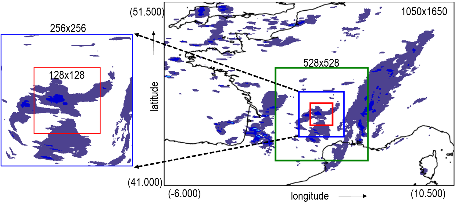
The second solution consists on partitioning the map into () patches and making predictions for each patch. However, these predictions are dependent. In fact, since clouds moves over time, the prediction of precipitation inside each patch depends on information in neighboring patches. Thus, neighborhood information should be included in each input patch and should be used for prediction. We propose an algorithm (Algorithm 1) to extract patches. It consists in interpolating the neighborhood information (the areas between the green rectangle and the red rectangle) and including this information inside the input patch (the area between the blue rectangle and the red rectangle) (Figure 3.(b)). Each area is interpolated independently. Since the near areas are more important for the prediction, the further away from the target patch (red rectangle), the more the size of the area to interpolate is increased (Figure 4).

(a) Full map resize
(b) Patch extraction

3.4 Data transformation and normalization
Considerable right skewness in precipitation distributions arises because of the relatively numerous occurrences of “no-rain” days (Skees & Shenton 1974). In fact, most precipitation values fall between and , see Fig. 5.(a). In general, right skewness should be reduced to make patterns in the data more interpretable and helps to meet the assumptions of inferential statistics (Gökmen 2015). For that, many transformations can be used such as log transformation, square root transformation and Box Cox(Box & Cox 1964). In our case, the “spike” of zeros all have the same value. Thus, no matter what transformation we apply, they are always going to have the same value. They are always going to be a “spike” sticking out from the rest of the distribution. Thus, we choose to apply log transformation to compress high values of precipitation (McCune & Grace 2002) and then to avoid that these values will be considered as noise by the neural network. In order to include zero values, we used instead of . Finally, we standardize all variables to have a mean of zero and a standard deviation of using z-score:
| (1) |

(a) original distribution

(b) root cube

(c) log(x+1)

(d) box cox
4 Models
The deterministic RNN-based model (Figure 6.(a)) is ConvLSTM (Xingjian et al. 2015). It follows “sequence to sequence” architecture. It consists of two networks, an encoding network and a decoding network. the initial states and cell outputs of the decoding network are copied from the last state of the encoding network. Both networks are formed by stacking several ConvLSTM layers. The encoder network consists of three stacked stride-1 convLSTM layers with 64, 192 and 192 filters, respectively. The filter size is for the three layers. We added a downsampling layer before each convLSTM layer. Each downsampling layer contains a stride-2 convolution followed by Leaky-ReLU non-linearity. The decoder network consists of three stacked stride-1 convLSTM layers with 192, 192 and 64 filters, respectively. The filter size is for the three layers. We added a upsampling layer after each convLSTM layer. Each downsampling layers contain a stride-2 deconvolution followed by Leaky-ReLU non-linearity. After the last dwonsampling layer, we added a stride-1 convolution followed by Leaky-ReLU non-linearity and a stride-1 convolution convolutional layer to generate the final prediction.
The stochastic RNN-based model (Figure 6.(b)) is SVG-LP (Denton & Fergus 2018). The predictor network is a two layer LSTMs with cells in each layer. The posterior and prior networks are both single layer LSTMs with cells in each layer. Each network has a linear embedding layer and a fully connected output layer. The output dimensionalities of the LSTM networks are ; . The encoder and decoder has the same architecture of the proposed U-net. We replaced the last layer of encoder by a stride-1 convolution followed by batch normalization and tanh nonlinearity. The encoder outputs a vector with dimensionality . We added a deconvolution at the beginning of the decoder to output feature maps with a size. This model follows “sequence modeling” architecture also named “one to many” architecture used in natural language processing (NLP). To generate a sequence of images (the future), we give the first images (the past) as input to the network. Starting from time step, the generated output is passed as input into the next time step.
The CNN-based model (Figure 6.(c)) follows an encoder-decoder architecture of U-net network with skip connections (Ronneberger et al. 2015). In this work, the encoder includes five convolutional layers. The first four convolutional layers are each followed by a downsampling layer that decrease the size of the output feature maps. The first two convolutional layer use two convolutions. The remaining convolutional layers use three convolutions. The encoder outputs feature maps with a size. The decoder uses four upsampling layers each followed by a convolutional layer to construct an output image with the same resolution of the input one. The first two convolutional layers of decoder use three convolutions. The third convolutional layers of decoder use two convolutions. The last convolutional layer of decoder uses three convolutions to generate feature maps with a size then uses a convolution to produce the finals precipitation maps. The weights of the network are randomly initialized. Each convolution is followed by batch normalization and Leaky-ReLU non-linearity. The final convolution is followed by linear activation.

(a) deterministic RNN: ConvLSTM

(b) stochastic RNN: SVG-LP

(c) CNN: U-net
5 Loss function
The network have to learn to produce images having the same structure as ground truth images. This goal can be achieved by using loss function that preserves the structure as is the case with SSIM loss. SSIM score (Wang et al. 2004) is used to measure the similarity of structure between the two images, rather than a pixel-to-pixel difference like the PSNR does for example. It is computed between two windows and in the image. It is given by (2) which combines three comparative measures: luminance (3), contrast (4) and structure (5).
| (2) |
where they set
| (3) |
where to stabilize the division with weak denominator, is the dynamic range of the pixel-values, .
| (4) |
where to stabilize the division with weak denominator, is the dynamic range of the pixel-values, .
| (5) |
where used to stabilize the division with weak denominator.
In SSIM paper (Wang et al. 2004), in order to evaluate the overall image quality, the mean SSIM score, an uniformly weighted average of the different window scores is defined as:
| (6) |
where and are the reference and the distorted images, respectively; and and are the image contents at the jth local window; and is the number of local windows of the image. However, there is high class imbalance: about of the pixels have no precipitation. Thus, with an uniformly weighted loss function, each window contributes equally to the loss function, and a network can achieve high accuracy by simply predicting the dominant class for all pixels. To improve upon this situation, we use a weighted loss calculation in which the loss for each window is weighted based on its standard deviation. We compute a weighted average of the different windows in the image:
| (7) |
where , is the standard deviation of the window . For each target window , the greater its standard deviation , the greater the variation between its pixels, the greater its weight . If does not contain precipitation, then and . The weighted SSIM loss is defined as :
| (8) |
Similarly, we propose a weighted version of the MSE loss that reduces the influence of zero value pixels in precipitation maps:
| (9) |
where and are the reference and the generated images respectively; and and are their ith pixels respectively; and is the number of pixel in each image, if , otherwise; is the “rain/no-rain” threshold.
On the one hand, the weighted SSIM loss preserves the structure and contrast in high-frequency regions better than the weighted MSE loss . On the other hand, preserves colors and luminance better than . To capture the best characteristics of both error functions, we propose to combine them:
| (10) |
We empirically set . Finally, we have added the regularization term to the loss. Regularization term penalize all the weights of the network by making them small making the model simpler and avoiding overfitting.
| (11) |
where is the penalty term for regularization parameter which determines how much to penalizes the weights; in the number of the weights in the network.
6 Experiments
The models are trained on radar images each, sampled every 15 minutes, with the aim to forecast the next images, i.e. up to 1 1/2 hours in the future. The models are implemented in Pytorch. Initial training was done using one NVIDIA T4 GPU on the interactive Google Colab platform, production runs were carried out using one NVIDIA Tesla K80 GPU. Training was done using the Adam optimizer with a learning rate of . In Figure 7, we show learning curve of U-net model.

For evaluation, we compute (mae) and (f1 score) over the test data for each of the frames for every prediction. The (mae) metric is defined as the absolute error between the predicted precipitation and the ground truth. The (f1 score) is calculated from the precision and recall and is commonly used by machine learning researchers. To compute (f1 score), we convert the prediction and ground truth to a 0/1 matrix using thresholds of and precipitation rate.
6.1 Evaluation of loss function
In Figure 8, we show the last output frame (+1h30) of the U-net model using different loss functions. As seen in Figure 8.(b) and Figure 8.(d), the use of weighting in WMSE and WSSIM allows the network to generate more precipitation. Comparing to WMSE, WSSIM loss allows the network to generate highest values of precipitation (). as seen in Figure 8.(d), these high values are predicted in the right places comparing to the ground truth image. This can be seen also in (Figure 9.(b)); where the curve of WSSIM loss achieves the highest score of (f1 score) with threshold . However, WSSIM loss spreads less precipitation in the map comparing to WMSE loss. This can be seen in (Figure 9.(c)); where the curve of WSSIM have the highest score of (mae). This justifies the need to combine WSSIM with WMSE losses (Figure 8.(e)).

(a) mse loss

(b) wmse loss

(c) ssim loss


(d) wssim loss

(e) wssim+wmse loss

(f) GT

(a)

(b)

(c)
6.2 Evaluation of patch extraction method
For the patch extraction algorithm, we fixed , , and . The size of the interpolated neighboring area is pixels around the target patch. To study the impact of adding neighborhood information to the patch, we compare two U-net models that take patches as inputs. In the first model, full images are divided into patches of size . Since the target patch size is , then the size of neighbouring region is equal to the margin which is equal to pixels. In the second model, we use patch extraction method to get patches of . In this model, the margin is also equal to pixels. However, it summarizes neighboring information of an area of pixels around the target patch (Figure 4). As seen in Figure 10, the second model achieves best scores of (mae) and (f1 score).

(a)

(b)

(c)
6.3 Evaluation of models
In this section, we compare reconstruction quality of the three proposed models: U-net, ConvlSTM and SVG-LP. In Figure 12, we present two particular precipitation prediction for the proposed model, which include two types of precipitation. The models predicts 6 image maps in the future. As seen, the three models capture the essential evolution of the precipitation fields. The CNN-based method outperforms the RNN-based models. It is able to generate high value of precipitation. It can predict the future rainfall contour more accurately. It is mainly caused by the strong spatial correlation in the radar maps, i.e., the motion of clouds is highly consistent in a local region. Also, it can be seen that ConvLSTM outperforms SVG-LP. However, ConvLSTM network tends to blur later frames. The blurring effect of ConvLSTM may be caused by the inherent uncertainties of the task. This was one main motivation for the stochastic variational frame prediction method. SVG-LP model triggers more false alarms and is less precise than ConvLSTM. The evaluation scores of the three models are presented in Figure 11.

(a)

(b)

(c)


+15min


+30min


+45min


+1h


+1h15


+1h30
7 Conclusion
In this work, we formulate precipitation nowcasting issue as a video prediction problem where both input and prediction target are image sequences. We trained our models to perform a regression task rather than classification task. Thus, the proposed models generates continuous precipitation values. We evaluated three popular models used in the precipitation nowcasting literature, ConvLSTM, SVG-LP and U-net. We proposed an algorithm to extract patch from precipitation map while including neighboring information for each patch. We proposed a loss function to solve the blurry image issue and to reduce the influence of zero value pixels in precipitation maps. Experiments show that the proposed method captures spatiotemporal correlations and yields meaningful forecasts. In addition, the quantitative evaluation shows promising results.
References
- Adewoyin et al. (2020) Adewoyin, R., Dueben, P., Watson, P., He, Y., and Dutta, R. Tru-net: A deep learning approach to high resolution prediction of rainfall. arXiv preprint arXiv:2008.09090, 2020.
- Agrawal et al. (2019) Agrawal, S., Barrington, L., Bromberg, C., Burge, J., Gazen, C., and Hickey, J. Machine learning for precipitation nowcasting from radar images. arXiv preprint arXiv:1912.12132, 2019.
- Ayzel et al. (2019) Ayzel, G., Heistermann, M., Sorokin, A., Nikitin, O., and Lukyanova, O. All convolutional neural networks for radar-based precipitation nowcasting. Procedia Computer Science, 150:186–192, 2019.
- Ayzel et al. (2020) Ayzel, G., Scheffer, T., and Heistermann, M. Rainnet v1. 0: a convolutional neural network for radar-based precipitation nowcasting. Geoscientific Model Development, 13(6):2631–2644, 2020.
- Ballas et al. (2015) Ballas, N., Yao, L., Pal, C., and Courville, A. Delving deeper into convolutional networks for learning video representations. arXiv preprint arXiv:1511.06432, 2015.
- Bihlo (2019) Bihlo, A. Precipitation nowcasting using a stochastic variational frame predictor with learned prior distribution. arXiv preprint arXiv:1905.05037, 2019.
- Bonnet et al. (2020) Bonnet, S. M., Evsukoff, A., and Morales Rodriguez, C. A. Precipitation nowcasting with weather radar images and deep learning in são paulo, brasil. Atmosphere, 11(11):1157, 2020.
- Bowler et al. (2004) Bowler, N. E., Pierce, C. E., and Seed, A. Development of a precipitation nowcasting algorithm based upon optical flow techniques. Journal of Hydrology, 288(1-2):74–91, 2004.
- Box & Cox (1964) Box, G. E. and Cox, D. R. An analysis of transformations. Journal of the Royal Statistical Society: Series B (Methodological), 26(2):211–243, 1964.
- Cao et al. (2019) Cao, Y., Li, Q., Chen, L., Zhang, J., and Ma, L. Video prediction for precipitation nowcasting. arXiv preprint arXiv:1907.08069, 2019.
- Chen et al. (2020) Chen, L., Cao, Y., Ma, L., and Zhang, J. A deep learning-based methodology for precipitation nowcasting with radar. Earth and Space Science, 7(2):e2019EA000812, 2020.
- Chollet (2017) Chollet, F. Xception: Deep learning with depthwise separable convolutions. In Proceedings of the IEEE conference on computer vision and pattern recognition, pp. 1251–1258, 2017.
- Danielson & Gesch (2011) Danielson, J. J. and Gesch, D. B. Global multi-resolution terrain elevation data 2010 (GMTED2010). US Department of the Interior, US Geological Survey, 2011.
- Denton & Fergus (2018) Denton, E. and Fergus, R. Stochastic video generation with a learned prior. arXiv preprint arXiv:1802.07687, 2018.
- Franch et al. (2020) Franch, G., Nerini, D., Pendesini, M., Coviello, L., Jurman, G., and Furlanello, C. Precipitation nowcasting with orographic enhanced stacked generalization: Improving deep learning predictions on extreme events. Atmosphere, 11(3):267, 2020.
- (16) Gaur, Y., Jain, A., and Sarmonikas, G. Precipitation nowcasting using deep learning techniques.
- Gökmen (2015) Gökmen, V. Acrylamide in food: analysis, content and potential health effects. Academic Press, 2015.
- Hochreiter (1998) Hochreiter, S. The vanishing gradient problem during learning recurrent neural nets and problem solutions. International Journal of Uncertainty, Fuzziness and Knowledge-Based Systems, 6(02):107–116, 1998.
- Hochreiter & Schmidhuber (1997) Hochreiter, S. and Schmidhuber, J. Long short-term memory. Neural computation, 9(8):1735–1780, 1997.
- Kipf & Welling (2016) Kipf, T. N. and Welling, M. Semi-supervised classification with graph convolutional networks. arXiv preprint arXiv:1609.02907, 2016.
- Kumar et al. (2020) Kumar, A., Islam, T., Sekimoto, Y., Mattmann, C., and Wilson, B. Convcast: An embedded convolutional lstm based architecture for precipitation nowcasting using satellite data. Plos one, 15(3):e0230114, 2020.
- McCune & Grace (2002) McCune, B. and Grace, J. Analysis of ecological communities–mjm software. Gleneden Beach, Oregon, USA, 2002.
- Miao et al. (2020) Miao, K., Wang, W., Hu, R., Zhang, L., Zhang, Y., Wang, X., and Nian, F. Multimodal semisupervised deep graph learning for automatic precipitation nowcasting. Mathematical Problems in Engineering, 2020, 2020.
- Qiu et al. (2017) Qiu, M., Zhao, P., Zhang, K., Huang, J., Shi, X., Wang, X., and Chu, W. A short-term rainfall prediction model using multi-task convolutional neural networks. In 2017 IEEE International Conference on Data Mining (ICDM), pp. 395–404. IEEE, 2017.
- Ronneberger et al. (2015) Ronneberger, O., Fischer, P., and Brox, T. U-net: Convolutional networks for biomedical image segmentation. In International Conference on Medical image computing and computer-assisted intervention, pp. 234–241. Springer, 2015.
- Samsi et al. (2019) Samsi, S., Mattioli, C. J., and Veillette, M. S. Distributed deep learning for precipitation nowcasting. arXiv preprint arXiv:1908.10964, 2019.
- Sato et al. (2018) Sato, R., Kashima, H., and Yamamoto, T. Short-term precipitation prediction with skip-connected prednet. In International Conference on Artificial Neural Networks, pp. 373–382. Springer, 2018.
- Shi et al. (2017) Shi, X., Gao, Z., Lausen, L., Wang, H., Yeung, D.-Y., Wong, W.-k., and Woo, W.-c. Deep learning for precipitation nowcasting: A benchmark and a new model. In Advances in neural information processing systems, pp. 5617–5627, 2017.
- Skees & Shenton (1974) Skees, P. and Shenton, L. Comments on the statistical distribution of rainfall per period under various transformations. In Proc. Symp. Statistical Hydrology, USDA Misc. Publ, volume 1275, pp. 172–196, 1974.
- Socaci et al. (2020) Socaci, I. A., Czibula, G., Ionescu, V.-S., and Mihai, A. Xnow: A deep learning technique for nowcasting based on radar products’ values prediction. In 2020 IEEE 14th International Symposium on Applied Computational Intelligence and Informatics (SACI), pp. 000117–000122. IEEE, 2020.
- Springenberg et al. (2014) Springenberg, J. T., Dosovitskiy, A., Brox, T., and Riedmiller, M. Striving for simplicity: The all convolutional net. arXiv preprint arXiv:1412.6806, 2014.
- Tian et al. (2020) Tian, W., Yi, L., Liu, W., Huang, W., Ma, G., and Zhang, Y. Ground radar precipitation estimation with deep learning approaches in meteorological private cloud. Journal of Cloud Computing, 9:1–12, 2020.
- Tran & Song (2019) Tran, Q.-K. and Song, S.-k. Computer vision in precipitation nowcasting: Applying image quality assessment metrics for training deep neural networks. Atmosphere, 10(5):244, 2019.
- Trebing & Mehrkanoon (2020) Trebing, K. and Mehrkanoon, S. Smaat-unet: Precipitation nowcasting using a small attention-unet architecture. arXiv preprint arXiv:2007.04417, 2020.
- Wang et al. (2017) Wang, Y., Long, M., Wang, J., Gao, Z., and Philip, S. Y. Predrnn: Recurrent neural networks for predictive learning using spatiotemporal lstms. In Advances in Neural Information Processing Systems, pp. 879–888, 2017.
- Wang et al. (2018) Wang, Y., Gao, Z., Long, M., Wang, J., and Yu, P. S. Predrnn++: Towards a resolution of the deep-in-time dilemma in spatiotemporal predictive learning. arXiv preprint arXiv:1804.06300, 2018.
- Wang et al. (2004) Wang, Z., Bovik, A. C., Sheikh, H. R., and Simoncelli, E. P. Image quality assessment: from error visibility to structural similarity. IEEE transactions on image processing, 13(4):600–612, 2004.
- Xiang et al. (2020) Xiang, Y., Ma, J., and Wu, X. A precipitation nowcasting mechanism for real-world data based on machine learning. Mathematical Problems in Engineering, 2020, 2020.
- Xingjian et al. (2015) Xingjian, S., Chen, Z., Wang, H., Yeung, D.-Y., Wong, W.-K., and Woo, W.-c. Convolutional lstm network: A machine learning approach for precipitation nowcasting. In Advances in neural information processing systems, pp. 802–810, 2015.
- Yao et al. (2020) Yao, G., Liu, Z., Guo, X., Wei, C., Li, X., and Chen, Z. Prediction of weather radar images via a deep lstm for nowcasting. In 2020 International Joint Conference on Neural Networks (IJCNN), pp. 1–8. IEEE, 2020.