Improved Stability Estimates and Flight Time Predictions Using Higher-Order Transverse Discontinuity Mapping in Hybrid Dynamical Systems

Rohit Chawla Email: rohit.chawla@ucd.ie Affiliation: UCD Centre for Mechanics, Dynamical Systems and Risk Laboratory, School of Mechanical and Materials Engineering, University College Dublin, Dublin, Ireland Affiliation: UCD Energy Institute, University College Dublin, Dublin, Ireland Aasifa Rounak Email: aasifa.rounak@ucd.ie Affiliation: UCD Centre for Mechanics, Dynamical Systems and Risk Laboratory, School of Mechanical and Materials Engineering, University College Dublin, Dublin, Ireland Affiliation: UCD Energy Institute, University College Dublin, Dublin, Ireland Vikram Pakrashi Email: vikram.pakrashi@ucd.ie Affiliation: UCD Centre for Mechanics, Dynamical Systems and Risk Laboratory, School of Mechanical and Materials Engineering, University College Dublin, Dublin, Ireland Affiliation: UCD Energy Institute, University College Dublin, Dublin, Ireland Corresponding author: Corresponding author

Abstract

This article emphasizes on inconsistencies in the dynamical estimates obtained by first-order transverse discontinuity mapping (TDM) and direct numerical observations for hybrid dynamical systems. Pitfalls of locally linearizing hybrid nonlinear dynamical systems near discontinuity boundaries are demonstrated along with examples of how such linearization could lead to incorrect estimates of impact occurrences for transverse interactions with a rigid barrier. A higher-order TDM is proposed to overcome this shortcoming, allowing for better analytical estimation of impact occurrence times, state transitions, and, consequently, the evolution of trajectories. The difference in flight times of two closely initiated trajectories in the local neighbourhood of a discontinuity boundary is estimated up to $\mathcal{O}(2)$ . The resulting quadratic equation implies that the orbits local to the impacting state, corresponding to a negative discriminant, won’t reach the discontinuity boundary. Further, the $\mathcal{O}(2)$ correction terms to the analytical expression of the TDM ensure that the flight time estimates do not diverge for low-velocity impacts near grazing, thereby avoiding overestimation of the mapped state. A numerical method is subsequently developed to estimate a saltation matrix incorporating the proposed higher-order TDM to avoid incorrect impact occurrences. Modifications to the existing algorithms used to numerically quantify local stability, namely the Lyapunov spectra and Floquet multipliers, are proposed. Stability analyses using the proposed higher-order approach are carried out for representative cases of a hard impact oscillator and a pair impact oscillator, with results consistent with numerically obtained bifurcation diagrams.

Keywords:

Discontinuity mapping , Saltation matrix , Vibro-impact oscillators , Bifurcation analysis , Lyapunov exponents , Floquet analysis

Nomenclature

The mathematical symbols used throughout this paper are listed in Table 1.

Table 1: Description of mathematical symbols

Variable name	Symbols	Dims.
Scalars
Instant of impact state $\mathbf{x}_{i}$	$t_{i}$	$\mathbb{R}^{1}$
Discontinuity function	$H(\mathbf{x})$	$\mathbb{R}^{1}$
Flight time for $\mathbf{x}_{0}$ to reach $\Sigma_{2}$ at $\mathbf{x}_{2}$	$\delta$	$\mathbb{R}^{1}$
First-order flight time for $\mathbf{x}_{0}$ to reach $\Sigma_{2}$ at $\mathbf{x}_{2}$	$\delta_{1}$	$\mathbb{R}^{1}$
Positive root of the second-order flight time for $\mathbf{x}_{0}$ to reach $\Sigma_{2}$ at $\mathbf{x}_{2}$	$\delta_{+}$	$\mathbb{R}^{1}$
Negative root of the second-order flight time for $\mathbf{x}_{0}$ to reach $\Sigma_{2}$ at $\mathbf{x}_{2}$	$\delta_{-}$	$\mathbb{R}^{1}$
Components of perturbation state $\mathbf{y}\in\mathbb{R}^{n}$	$y_{i}$	$\mathbb{R}^{1}$
Scaling factor of perturbation state $\mathbf{y}$	$r_{0}$	$\mathbb{R}^{1}$
Quadratic function of flight time $\delta$	$G$	$\mathbb{R}^{1}$
Coefficient of restitution	$r$	$\mathbb{R}^{1}$
Components of reset map $\mathbf{R}(\mathbf{x}_{i})$	$r_{1,2}$	$\mathbb{R}^{1}$
Position component of the rigid barrier	$\sigma$	$\mathbb{R}^{1}$
Vectors
Generalized state	$\mathbf{x}$	$\mathbb{R}^{n}$
Generalized velocity vector field	$\mathbf{F}(\mathbf{x})$	$\mathbb{R}^{n}$
Perturbation to $\mathbf{x}$	$\mathbf{y}$	$\mathbb{R}^{n}$
Initial state $\mathbf{x}$ post transients on periodic orbit	$\mathbf{x}_{p}$	$\mathbb{R}^{n}$
Perturbation state to $\mathbf{x}_{p}$	$\hat{\mathbf{x}}$	$\mathbb{R}^{n}$
State $\mathbf{x}$ at impact	$\mathbf{x}_{i}$	$\mathbb{R}^{n}$
Reset map	$\mathbf{R}(\mathbf{x}_{i})$	$\mathbb{R}^{n}$
Perturbed state at impact	$\mathbf{x}_{0}$	$\mathbb{R}^{n}$
Perturbed state on $\Sigma_{2}$	$\mathbf{x}_{2}$	$\mathbb{R}^{n}$
Reset map of perturbed state $\mathbf{R}(\mathbf{x}_{2})\in\Sigma_{2}$	$\mathbf{x}_{3}$	$\mathbb{R}^{n}$
TDM of perturbed state	$\mathbf{x}_{4}$	$\mathbb{R}^{n}$
Perturbation state during impact	$\mathbf{y}_{-}$	$\mathbb{R}^{n}$
TDM of perturbation state	$\mathbf{y}_{+}$	$\mathbb{R}^{n}$
Matrices
Jacobian matrix of $\mathbf{F}$	$\nabla\mathbf{F}(\mathbf{x})^{T}$	$\mathbb{R}^{n\times n}$
Hessian matrix of $i^{th}$ component of $\mathbf{F}$	$H_{i}$	$\mathbb{R}^{n\times n}$
Hessian matrix of $i^{th}$ component of $\mathbf{R}$	$\tilde{H}_{i}$	$\mathbb{R}^{n\times n}$
First-order saltation matrix	$\mathbf{S}$	$\mathbb{R}^{n\times n}$
Higher-order saltation matrix	$\mathbf{S}_{2}$	$\mathbb{R}^{n\times n}$
Higher-order saltation matrix after $i^{th}$ impact	$\mathbf{S}^{i}_{2}$	$\mathbb{R}^{n\times n}$
Perturbation matrix at impact	$\mathbf{Y}_{-,\text{impact}}$	$\mathbb{R}^{n\times n}$
Perturbation matrix after impact	$\mathbf{Y}_{+,\text{impact}}$	$\mathbb{R}^{n\times n}$
State transition matrix before $i^{th}$ impact	$\mathbf{\Phi}_{i}$	$\mathbb{R}^{n\times n}$
Global state transition or monodromy matrix	$\mathbf{\Phi}$	$\mathbb{R}^{n\times n}$
Sets
Initial Poincaré section on periodic orbit	$\Sigma_{1}$	$\mathbb{R}^{n-1}$
Discontinuity boundary	$\Sigma_{2}$	$\mathbb{R}^{n-1}$

1 Introduction

Dynamical systems are often subjected to mechanical impacts, leading to possible compromise in performance and safety. These impacts arise due to wear and tear with limited clearance between components or loosened joints in a wide range of systems, including gear assemblies Kahraman and Singh 1990, Karagiannis and Pfeiffer 1991, impact print hammers Hendriks 1983, Tung and Shaw 1988, walking robots Holmes et al. 2006 and heat exchanger tubesGoyder and Teh 1989, Païdoussis and Li 1992. Similar effects occur in submerged and floating buoyant vessels impacting rigid harbours during ship grounding Virgin and Plaut 2009, Ibrahim 2014, Xue et al. 2023, metal cutting Wiercigroch and Budak 2001, drilling and milling Krivtsov and Wiercigroch 1999, Wiercigroch et al. 1999 and many-body interaction systems involving friction Feeny 1992, Fan et al. 2020. The dynamics of these systems are often analyzed using the canonical form of impact oscillators Shaw and Holmes 1983a, Shaw and Holmes 1983b, Bishop 1994, Jiang and Wiercigroch 2016, Luo and Chen 2005, Chillingworth and Nordmark 2013, Whiston 1987a, Whiston 1987b, Foale and Bishop 1992, Foale and Bishop 1994, Ma et al. 2006, mathematically modelled as piecewise-smooth (PWS) dynamical systems Bernardo et al. 2008, Awrejcewicz and Lamarque 2003, Belykh et al. 2023, Brogliato 1999. A wide range of theoretical Nordmark 1991, Nordmark 1992, Nusse and Yorke 1992, Simpson et al. 2020, Nordmark 1997, Ma et al. 2008 and experimental Wiercigroch and Sin 1998, Banerjee et al. 2009, Ing et al. 2006, Ing et al. 2008, Ing et al. 2010, Pavlovskaia et al. 2010 investigations of impact oscillators reveal occurrences of many dynamically rich phenomena, collectively known as discontinuity-induced bifurcations (DIBs) Bernardo et al. 2008. Some examples include period adding cascades Piiroinen et al. 2004, Oestreich et al. 1996, Oestreich et al. 1997, Popp et al. 1999, Shaw and Holmes 1983a, Fredriksson and Nordmark 2000, Rounak and Gupta 2020, grazing bifurcations Banerjee et al. 2009, Jiang et al. 2017, Chin et al. 1994, sliding motion Di Bernardo et al. 2002, chattering sequence Budd and Dux 1994, narrow band and robust chaos Banerjee et al. 2009, Thompson and Ghaffari 1983, Hassouneh et al. 2004 and coexisting attractors Chawla et al. 2024. Unstable, chaotic vibrations resulting from DIBs can be undesirable or harmful for safety or performance, making their analysis essential for the design, performance and control.

DIBs primarily occur when an orbit grazes the discontinuity boundary Bernardo et al. 2008. Nordmark Nordmark 1991 showed that in such conditions, orbits near the discontinuity boundary stretch in the phase space, resulting in large amplitude oscillations known as square-root singularity. Away from this grazing condition, the evolution of perturbations near the discontinuity boundary is determined by a transverse discontinuity mapping (TDM) Bernardo et al. 2008. Fredriksson and Nordmark Fredriksson and Nordmark 2000 had derived the normal form of the TDM using first-order approximations. This TDM depends on the time taken for orbits to reach the discontinuity boundary. For an $n$ dimensional hybrid dynamical system $\mathbf{x}\in\mathbb{R}^{n}$ obeying $\dot{\mathbf{x}}=\mathbf{F}(\mathbf{x},\mathbf{u},t)$ , a first-order Taylor series expansion Fredriksson and Nordmark 2000, Leine 2000 approximates the time difference $\delta_{1}$ between impacts as

\delta_{1}=-\frac{\nabla H(\mathbf{x}_{i})^{T}\cdot\mathbf{y}_{-}}{\nabla H(\mathbf{x}_{i})^{T}\cdot\mathbf{F}(\mathbf{x}_{i})}

(1)

where $\mathbf{F}(\mathbf{x},\mathbf{u},t)$ is the governing vector field, $\mathbf{u}$ are parameters of the system and overdot represents derivative with respect to time $t$ . The discontinuity boundary $\mathbf{\Sigma_{2}}$ is modelled by a scalar function $H(\mathbf{x})$ satisfying $\Sigma_{2}=\{\mathbf{x}_{i}\in\mathbb{R}^{n}:H(\mathbf{x}_{i})=0\}$ and $\mathbf{y}_{-}$ is the perturbation vector during an impact of the primary state at $\mathbf{x}(t_{i})=\mathbf{x}_{i}$ ; $t_{i}$ being the instant of impact.

This first-order flight time $\delta_{1}$ has an inherent problem. The flight time $\delta_{1}$ in Eq. (1) is a real-valued fraction that assumes all perturbations in the local neighbourhood of an impact state $\mathbf{x}_{i}$ , reaches the discontinuity bondary and gets mapped to $\mathbf{y}_{+}=\mathbf{S}\cdot\mathbf{y}_{-}$ while the primary state is mapped to $\mathbf{x}_{i}\rightarrow\mathbf{R}(\mathbf{x}_{i})$ via the impact map $\mathbf{R}(\mathbf{x})$ . Here, $\mathbf{S}$ , known as the saltation matrix, is the first-order TDM Fredriksson and Nordmark 2000, Leine 2000. The saltation matrix is essentially a state-transition matrix between perturbation vectors before and after impact, i.e., $\mathbf{y}_{-}$ and $\mathbf{y}_{+}$ . Additionally, another drawback of the first-order approximation of the flight time and the saltation matrix is that for low-velocity incidence and grazing orbits, the TDM gets stretched since the denominator diverges as $\nabla H(\mathbf{x}_{i})^{T}\cdot\mathbf{F}(\mathbf{x}_{i})=0$ . This also results in overestimating the mapped state away from the discontinuity boundary.

This paper first demonstrates how impacts are incorrectly predicted for certain perturbations in the local neighbourhood of the discontinuity boundary. Specifically, the first-order approximation of the flight time $\delta_{1}$ and the saltation matrix $\mathbf{S}$ fails to account for cases where the perturbed orbit misses the discontinuity boundary. Next, this work addresses this shortcoming by considering a higher-order Taylor series approximation to derive the flight time $\delta$ and TDM. This results in a quadratic equation in $\delta$ , implying that perturbations reach the discontinuity boundary only when the discriminant of the quadratic equation is non-negative, and is given by the real positive root $\delta_{+}$ . The positive root of the derived higher-order flight time estimate comprises additional terms in the denominator that ensure that the TDM does not diverge for low-velocity impacts close to the grazing condition. The correction terms, not present in the first-order saltation matrix, ensure that the mapped state post-impact is not overestimated for low-velocity impacts and reaches the discontinuity boundary correctly. These limitations have been overlooked mainly because the existing literature focuses on discontinuity mappings near grazing like the zero-time (ZDM) Yin et al. 2018, Kundu et al. 2012 and Poincaré section discontinuity map (PDM) di Bernardo et al. 2001, Di Bernardo et al. 2002, Di Bernardo et al. 2001, Simpson et al. 2020. Additionally, the current literature Bernardo et al. 2008 on higher-order approximations of the TDM relies on the first-order flight time $\delta_{1}$ . A singularity is unavoidable in the first-order flight time due to the denominator of Eq. (1) for low-velocity impacts. Discrepancies between dynamical behaviour derived from mapping techniques and direct numerical simulations become evident in complex, chaotic dynamics, degenerate bifurcations, or higher co-dimensional bifurcations Yin et al. 2018. This article resolves the discrepancy by deriving the TDM by combining a higher-order quadratic form of $\delta_{+}$ and a higher-order Taylor series approximation of the perturbed state in the local neighbourhood of $\mathbf{x}_{i}$ .

Next, a higher-order TDM derived in this article poses a new challenge. Since the mapped state $\mathbf{y}_{+}$ is proportional to terms like $\delta^{2}_{+}$ , $\mathbf{y}_{-}\cdot\mathbf{y}_{-}$ , and $\delta_{+}\mathbf{y}_{-}$ , the TDM cannot be expressed as a state transition or saltation matrix like $\mathbf{S}\cdot\mathbf{y}_{-}$ . Hence, a higher-order saltation matrix comprising quadratic terms cannot be expressed in a closed analytical form, and estimation of monodromy matrices and Floquet multipliers for stability analysis becomes difficult. This work addresses the problem by introducing a method to numerically obtain the saltation matrix comprising higher-order correction terms compatible with the first-order variational equation.

Incorrect estimation of impact occurrences using the first-order TDM has significant consequences for stability analysis based on Floquet multipliers Floquet 1883, Nayfeh and Balachandran 2008 and Lyapunov exponents (LEs) Oseledec 1968, Pesin 1977, Benettin et al. 1980, Bennetin et al. 1980. The monodromy matrix comprises products of state transition and saltation matrices multiplied in their order of occurrence. Any incorrect prediction of the occurrence of an impact alters the monodromy matrix, resulting in an inaccurate representation of the perturbation dynamics near the discontinuity boundary. Consequently, using a first-order linearization instead of the proposed higher-order approach may result in misleading conclusions regarding orbital stability. Moreover, when the time between two consecutive impacts is large, the separation between nearby orbits can increase, potentially causing the perturbation vector to miss the discontinuity boundary while the primary orbit undergoes an impact. In such cases, the monodromy matrix should remain unaffected, as no saltation matrix should be applied. However, the first-order TDM, which assumes a real-valued flight time, cannot capture this scenario. In contrast, a higher-order TDM and saltation matrix correctly predicts when impacts occur. This ensures an accurate monodromy matrix and its corresponding Floquet multipliers.

Similarly, the computation of LEs in hybrid dynamical systems depends on the first-order TDM and saltation matrix Lamba and Budd 1994, Müller 1995, De Souza and Caldas 2004, Jin et al. 2006, Leine 2012, Mandal et al. 2013, Stefanski 2000, Stefanski et al. 2005, Dabrowski 2012, Li et al. 2018, Balcerzak et al. 2020. In impact oscillators, LEs are typically calculated after multiple impacts to eliminate transient effects. Therefore, an incorrect prediction of an impact of the perturbation vector accumulates over successive applications of the first-order saltation matrix, resulting in less accurate perturbation dynamics. Instead, the higher-order TDM provides better estimates of the true behaviour of perturbed orbits near the discontinuity boundary.

This paper thus presents a generalized method to calculate the flight times for impact of orbits in the local neighbourhood of the discontinuity boundary and the corresponding TDM by incorporating higher-order corrections terms up to $\mathcal{O}(\delta_{+}^{2},\delta_{+}\mathbf{y}_{-},\mathbf{y}_{-}\cdot\mathbf{y}_{-})$ . The derivations can be extended to accommodate correction terms greater than $\mathcal{O}(2)$ if necessary, following the approach presented here, and subsequently applied to autonomous and non-autonomous hybrid systems with multiple barriers. Next, this article proposes a method to obtain higher-order saltation matrices numerically. The higher-order TDMs are validated by conducting a stability analysis of impact oscillators with multiple barriers using Floquet multipliers and LEs.

The article is structured as follows. In Sec. 2, the higher-order TDM for a hybrid dynamical system is derived. Section 3 compares the higher-order results with the first-order linearized approaches for two representative impact oscillators with multiple impacts. In Sec. 4, the higher-order TDM is implemented to obtain the Lyapunov spectrum. Section 5 presents the methodology to numerically evaluate a higher-order saltation matrix. Section 6 presents a method to construct a monodromy matrix using the higher-order saltation matrix, followed by an eigenvalue analysis of the respective impact oscillators. Section 7 investigates the stability analysis of the impact oscillator for which period-adding cascades are observed. Section 8 summarises the principal outcomes of this study.

2 Mathematical formulation

The generalized form of a dynamical system represented by the state $\mathbf{x}(t)$ , where $\mathbf{x}\in\mathbb{R}^{n}$ , and its corresponding variational form, post transients, can be expressed in the state space form as

	$\displaystyle\dfrac{d\mathbf{x}}{dt}$	$\displaystyle=\mathbf{F}(\mathbf{x}),$		(2)
	$\displaystyle\dfrac{d\mathbf{y}}{dt}$	$\displaystyle\approx\mathbf{\nabla}\mathbf{F}(\mathbf{x})^{T}\cdot\mathbf{y}+\mathcal{O}(\|\|\mathbf{y}\|\|^{2})$

where $\mathbf{y}$ is a perturbation to the state $\mathbf{x}$ . The variational form governs the dynamics of orbits in the local neighbourhood of $\mathbf{x}$ and is derived using first-order Taylor approximations. The state space form is also valid for a non-autonomous system with explicit time dependence, i.e., $\mathbf{F}(\mathbf{x},t)$ . The additional phase variable, $t$ , can be included in $\mathbf{x}$ such that $\dot{t}=1$ , making the new state $\mathbf{x}^{\prime}$ $n+1$ dimensional. Therefore, the derivations presented in this section apply to both autonomous and non-autonomous systems. In general, for PWS systems, nearby perturbed trajectories reach the discontinuity boundary at different instants of time (see Fig. 1). Implementing a linearized TDM to estimate flight times can result in overestimating the mapped perturbed state near the discontinuity boundary. Higher-order terms must be considered to accurately map perturbed trajectories for low-velocity impacts, as demonstrated below.

The evolution of two nearby trajectories is depicted in the simplistic case of a 2-dimensional state space (Fig. 1). Two closely spaced states $\mathbf{x}_{p}$ and $\mathbf{\hat{x}}$ are initiated together from the Poincaré section $\Sigma_{1}$ . Here, $\mathbf{\hat{x}}$ represents a perturbed trajectory from $\mathbf{x}_{p}$ , i.e. $\mathbf{\hat{x}}=\mathbf{x}_{p}+\mathbf{y}$ , where $\mathbf{y}$ is an infinitesimal perturbation. After evolving in time, at $t=t_{i}$ , the orbit $\mathbf{x}_{p}$ impacts the rigid surface represented by the discontinuity boundary $\Sigma_{2}$ at $\mathbf{x}_{i}$ . At this instant, when the orbit, initiated from $\mathbf{x}_{p}$ impacts the surface $\Sigma_{2}=\{\mathbf{x}_{i}\in\mathbb{R}^{n}:H(\mathbf{x}_{i})=0\}$ , the trajectory gets mapped to $\mathbf{R}(\mathbf{x}_{i})$ . Here, $\mathbf{R}(\mathbf{x})$ is an impact map based on a restitutive law, whereas $H(\mathbf{x})=0$ models the impacting condition. The impact or reset map $\mathbf{R}(\mathbf{x})$ is a typical example of a non-smooth event that arises in PWS dynamical systems. Applying the impact map $\mathbf{R}(\mathbf{x}_{0})$ to the perturbed trajectory $\mathbf{\hat{x}}(t_{i})=\mathbf{x}_{0}$ at the instant of impact $t_{i}$ will result in an incorrect prediction of state since $\mathbf{x}_{0}$ has not yet reached the impacting surface $\Sigma_{2}$ at $t_{i}$ . Thus, the difference in the flight times of the two paths $\mathbf{x}_{i}$ and $\mathbf{x}_{0}$ needs to be considered. The corresponding derivation of the flight time with higher-order approximations, is obtained next. Using the flight time difference, a higher-order TDM is derived, that accurately maps the state $\mathbf{x}_{0}$ to $\mathbf{x}_{4}$ . It is important to note that $\mathbf{x}_{4}$ now lies in the forbidden region $H(\mathbf{x})<0$ but eventually evolves in time to reach the barrier at $H(\mathbf{x}_{3})=0$ . Post impact, the perturbed trajectory when initiated at $\mathbf{x}_{4}$ , would take the same flight time to arrive at $\mathbf{x}_{3}$ on $\Sigma_{2}$ as the perturbed trajectory at $\mathbf{x}_{0}$ would take to reach $\mathbf{x}_{2}$ , followed by the mapping $\mathbf{R}(\mathbf{x}_{2})$ on $\Sigma_{2}$ to reach $\mathbf{x}_{3}$ . This ensures that local trajectories obey a zero-time mapping to the discontinuity boundary, and the time difference is conserved. The mapping of the perturbed path from $\mathbf{x}_{0}$ to $\mathbf{x}_{4}$ at the instant of the impact of the unperturbed trajectory is the required TDM; see Fig. 1. The saltation matrix is essentially a first-order approximation of the state transition from $\mathbf{x}_{0}$ to $\mathbf{x}_{4}$ . A higher-order approximation of the flight time and the TDM is presented next.

Refer to caption — Figure 1: A schematic of phase portraits of two nearby trajectories exhibiting impact at $\Sigma_{2}$ . The blue line shows the actual trajectory. The red dashed line denotes the perturbed trajectory. The horizontal black dashed line $\Sigma_{1}$ denotes the section from which both the trajectories are initiated, and $\Sigma_{2}$ denotes the discontinuity boundary. The amber line denotes the perturbation vector.

Let $t_{i}$ represent the instant of the impact of the unperturbed trajectory. A Taylor expansion of $\mathbf{x}(t)$ about $t=t_{i}$ and $\mathbf{F}(\mathbf{x})$ about $\mathbf{x}=\mathbf{x}_{0}$ up to $\mathcal{O}(2)$ gives Eqs. 3 and (4).

\displaystyle\mathbf{x}(t)=\mathbf{x}(t_{i})+\Delta t\ \mathbf{F}(\mathbf{x}_{0})+\dfrac{1}{2}\Delta t^{2}\ \mathbf{\nabla}\mathbf{F}(\mathbf{x}(t_{i}))^{T}\cdot\mathbf{F}(\mathbf{x}(t_{i}))+\mathcal{O}(3)

(3)

\displaystyle\mathbf{F}(\mathbf{x})=\mathbf{F}(\mathbf{x}_{0})+\mathbf{\nabla}\mathbf{F}(\mathbf{x}_{0})^{T}\cdot\mathbf{\Delta x}+\dfrac{1}{2}\begin{bmatrix}\mathbf{\Delta x}^{T}\cdot H_{1}\cdot\mathbf{\Delta x}\\ \mathbf{\Delta x}^{T}\cdot H_{2}\cdot\mathbf{\Delta x}\\ \end{bmatrix}+\mathcal{O}(3)

(4)

Here, $H_{1}$ and $H_{2}$ denote the Hessian matrices of each component $f_{i}(\mathbf{x})$ of $\mathbf{F}(\mathbf{x})$ i.e., $H_{i}$ defined as the Jacobian of $\mathbf{\nabla}f_{i}(\mathbf{x})$ or $\mathbf{\nabla}(\mathbf{\nabla}f_{i}(\mathbf{x}))^{T}$ . Let $\delta$ be the time taken for the perturbed trajectory $\mathbf{\hat{x}}$ to reach impact surface $\Sigma_{2}$ from $\mathbf{x}(t_{i})=\mathbf{x}_{0}$ to $\mathbf{x}(t_{i}+\delta)=\mathbf{x}_{2}$ . Therefore, $\mathbf{x}_{2}$ is approximated by taking a Taylor expansion of $\mathbf{\hat{x}}$ along path 2 about $t=t_{i}$ (i.e., $\mathbf{x}(t_{i})=\mathbf{x}_{0})$ evaluated at $t=t_{i}+\delta$ up to $\mathcal{O}(2)$ giving

\displaystyle\mathbf{x}_{2}=\mathbf{x}_{0}+\delta\ \mathbf{F}(\mathbf{x}_{0})+\dfrac{1}{2}\delta^{2}\ \mathbf{\nabla}\mathbf{F}(\mathbf{x}_{0})^{T}\cdot\mathbf{F}(\mathbf{x}_{0})+\mathcal{O}(3)

(5)

$\mathbf{F}(\mathbf{x}_{0})$ in Eq. (5) is approximated by a Taylor expansion of $\mathbf{F}(\mathbf{x})$ along path 1 about $\mathbf{x}_{i}$ and evaluated at $\mathbf{x}=\mathbf{x}_{0}$ . Retaining terms up to $\mathcal{O}(2)$ , $\mathbf{x}_{2}$ becomes Eq. (6)

\displaystyle\mathbf{x}_{2}=\mathbf{x}_{0}+\delta\ [\mathbf{F}(\mathbf{x}_{i})+\mathbf{\nabla}\mathbf{F}(\mathbf{x}_{i})^{T}\cdot\mathbf{y}_{-}]+\dfrac{1}{2}\delta^{2}\ \mathbf{\nabla}\mathbf{F}(\mathbf{x}_{i})^{T}\cdot\mathbf{F}(\mathbf{x}_{i})+\mathcal{O}(3)

(6)

where $\mathbf{y}_{-}$ is the perturbation vector at the instant of impact (i.e. $\mathbf{x}_{0}=\mathbf{x}_{i}+\mathbf{y}_{-}$ ).

Theorem 2.1

For all $\mathbf{x}_{i}\in\Sigma_{2}$ at $t_{i}$ , the flight time $\delta$ taken by $\mathbf{y}_{-}$ to reach $\mathbf{x}_{2}\in\Sigma_{2}$ satisfies the quadratic equation, $G(\delta,\mathbf{x}_{i},\mathbf{y}_{-})=A\delta^{2}+B\delta+C=0$ where the scalars $A$ , $B$ , $C$ are defined as

$\displaystyle A$	$\displaystyle=\mathbf{\nabla}H(\mathbf{x}_{i})^{T}\cdot\mathbf{\nabla}\mathbf{F}(\mathbf{x}_{i})^{T}\cdot\mathbf{F}(\mathbf{x})+\mathbf{F}(\mathbf{x}_{i})^{T}\cdot\mathbf{\nabla}(\mathbf{\nabla}H(\mathbf{x}_{i}))^{T}\cdot\mathbf{F}(\mathbf{x}_{i}),$	(7)
$\displaystyle B$	$\displaystyle=2\mathbf{\nabla}H(\mathbf{x}_{i})^{T}\cdot\mathbf{F}(\mathbf{x}_{i})+2\mathbf{\nabla}H(\mathbf{x}_{i})^{T}\cdot\mathbf{\nabla}\mathbf{F}(\mathbf{x}_{i})^{T}\cdot\mathbf{y}+\mathbf{y}^{T}\cdot\mathbf{\nabla}(\mathbf{\nabla}H(\mathbf{x}_{i}))^{T}\cdot\mathbf{F}(\mathbf{x}_{i})+\mathbf{F}(\mathbf{x}_{i})^{T}\cdot\mathbf{\nabla}(\mathbf{\nabla}H(\mathbf{x}_{i}))^{T}\cdot\mathbf{y},$
$\displaystyle C$	$\displaystyle=\mathbf{y}^{T}\cdot\mathbf{\nabla}(\mathbf{\nabla}H(\mathbf{x}_{i}))^{T}\cdot\mathbf{y}+2\mathbf{\nabla}H(\mathbf{x}_{i})^{T}\cdot\mathbf{y}.$

Proof. The equation for the impacting surface $H(\mathbf{x})$ expanded about the state at impact $\mathbf{x}_{i}$ up to $\mathcal{O}(2)$ and evaluated at $\mathbf{x}=\mathbf{x}_{2}$ is given by

\displaystyle H(\mathbf{x}_{2})=\ H(\mathbf{x}_{i})+\mathbf{\nabla}H(\mathbf{x}_{i})^{T}\cdot(\mathbf{x}_{2}-\mathbf{x}_{i})+\dfrac{1}{2}(\mathbf{x}_{2}-\mathbf{x}_{i})^{T}\cdot\mathbf{\nabla}(\mathbf{\nabla}H)^{T}\cdot(\mathbf{x}_{2}-\mathbf{x}_{i})+\mathcal{O}(3)

(8)

Substituting Eq. (6) in Eq. (8) and equating $H(\mathbf{x}_{i})=H(\mathbf{x}_{2})=0$ (since $\mathbf{x}_{i}$ and $\mathbf{x}_{2}$ lie on the impacting surface $\Sigma_{2}$ ), the time difference in impact between two closely spaced trajectories, i.e. $\delta$ can be solved up to $\mathcal{O}(2)$ . This results in a quadratic equation in $\delta$ given by

$\displaystyle\delta^{2}\Big($	$\displaystyle\mathbf{\nabla}H(\mathbf{x}_{i})^{T}\cdot\mathbf{\nabla}\mathbf{F}(\mathbf{x}_{i})^{T}\cdot\mathbf{F}(\mathbf{x})+\mathbf{F}(\mathbf{x}_{i})^{T}\cdot\mathbf{\nabla}(\mathbf{\nabla}H(\mathbf{x}_{i}))^{T}\cdot\mathbf{F}(\mathbf{x}_{i})\Big)+\delta\Big(2\mathbf{\nabla}H(\mathbf{x}_{i})^{T}\cdot\mathbf{F}(\mathbf{x}_{i})$	(9)
	$\displaystyle+2\mathbf{\nabla}H(\mathbf{x}_{i})^{T}\cdot\mathbf{\nabla}\mathbf{F}(\mathbf{x}_{i})^{T}\cdot\mathbf{y}+\mathbf{y}^{T}\cdot\mathbf{\nabla}(\mathbf{\nabla}H(\mathbf{x}_{i}))^{T}\cdot\mathbf{F}(\mathbf{x}_{i})+\mathbf{F}(\mathbf{x}_{i})^{T}\cdot\mathbf{\nabla}(\mathbf{\nabla}H(\mathbf{x}_{i}))^{T}\cdot\mathbf{y}\Big)$
	$\displaystyle\quad+\mathbf{y}^{T}\cdot\mathbf{\nabla}(\mathbf{\nabla}H(\mathbf{x}_{i}))^{T}\cdot\mathbf{y}+2\mathbf{\nabla}H(\mathbf{x}_{i})^{T}\cdot\mathbf{y}+\mathcal{O}(3)=G(\delta,\mathbf{x}_{i},\mathbf{y}_{-})=0$

$\blacksquare$

Lemma 2.2

The perturbed state $\mathbf{x}_{i}+\mathbf{y_{-}}$ reaches the discontinuity boundary $\Sigma_{2}=\{\mathbf{x}\in\mathbb{R}^{n}:H(\mathbf{x})=0\}$ , i.e., there exists a $\mathbf{x}_{2}\in\Sigma_{2}$ , after the flight time $\delta$ iff the quadratic equation $G(\delta,\mathbf{x}_{i},\mathbf{y}_{-})=A\delta^{2}+B\delta+C=0$ has a real solution. This is ensured by the discriminant condition, i.e., $B^{2}\geq 4AC$ . In this case, the discriminant is non-negative, ensuring $\delta\in\mathbb{R}$ ; otherwise, $\delta$ is imaginary and no impact occurs.

Lemma 2.3

When $B^{2}\geq 4AC$ , the flight time is given by the positive root of $G(\delta,\mathbf{x}_{i},\mathbf{y}_{-})=0$ , i.e.,

\delta_{+}=-\frac{B}{2A}\Bigg(1-\sqrt{1-\frac{4AC}{B^{2}}}\Bigg).

(10)

Proof. The roots of $G(\delta,\mathbf{x}_{i},\mathbf{y}_{-})=0$ are given by the solution $-\dfrac{B}{2A}\bigg(1\pm\sqrt{1-\dfrac{4AC}{B^{2}}}\bigg)$ that ensures that $H(\mathbf{x}_{2})=0$ and implies that perturbed trajectories reach the discontinuity boundary after time $t_{i}+\delta$ . Only the positive root of $\delta$ captures the limiting case when $\mathbf{x}_{2}\rightarrow\mathbf{x}_{i}$ when $\mathbf{y}_{-}\rightarrow 0$ and, hence, $\delta_{+}\rightarrow 0$ . $\blacksquare$

A comparison of Eq. (9) with Eq. (1) highlights two essential features. First, imaginary roots of Eq. (9) can exist and would imply that the perturbed orbits do not reach the discontinuity boundary. This contradicts the results of the first-order approximation of $\delta$ . Second, the magnitude of the perturbation vector $\mathbf{y}_{-}$ should lie within a critical range, which has been described in the later paragraphs, for impacts to occur. This critical range is obtained from the condition $B^{2}\geq 4AC$ that ensures that the discriminant of Eq. (10) is non-negative. Therefore, the correct flight time is given by the positive root of $G(\delta,\mathbf{x}_{i},\mathbf{y}_{-})=0$ . Geometrically, the discriminant condition suggests that when perturbation vectors become too large, they do not reach the discontinuity boundary and continue evolving in the region where $H(\mathbf{x})>0$ . On the contrary, the first-order approximation in $\delta=\delta_{1}$ predicts that impacts occur for all perturbations. Therefore, this phenomenon cannot be captured while implementing a linearized approximation of the TDM.

Theorem 2.4

At the impact time $t_{i}$ , the perturbed state $\mathbf{x}_{0}$ is mapped to the post-impact state $\mathbf{x}_{4}$ given by the higher-order TDM,

$\displaystyle\mathbf{x}_{4}=\mathbf{R}(\mathbf{x}_{i})$	$\displaystyle+\mathbf{\nabla}\mathbf{R}(\mathbf{x}_{i})^{T}\cdot\mathbf{y}_{-}+\delta_{+}\mathbf{\nabla}\mathbf{R}(\mathbf{x}_{i})^{T}\cdot\mathbf{F}(\mathbf{x}_{i})-\delta_{+}\mathbf{F}(\mathbf{R}(\mathbf{x}_{i}))+\delta_{+}\mathbf{\nabla}\mathbf{R}(\mathbf{x}_{i})^{T}\cdot\mathbf{\nabla}\mathbf{F}(\mathbf{x}_{i})^{T}\cdot\mathbf{y}_{-}$	(11)
	$\displaystyle+\dfrac{1}{2}\delta_{+}^{2}\mathbf{\nabla}\mathbf{R}(\mathbf{x}_{i})^{T}\cdot\mathbf{\nabla}\mathbf{F}(\mathbf{x}_{i})^{T}\cdot\mathbf{F}(\mathbf{x}_{i})-\delta_{+}\mathbf{\nabla}\mathbf{F}(\mathbf{R}(\mathbf{x}_{i}))^{T}\cdot\mathbf{\nabla}\mathbf{R}(\mathbf{x}_{i})^{T}\cdot\mathbf{y}_{-}$
	$\displaystyle\quad-\delta_{+}^{2}\mathbf{\nabla}\mathbf{F}(\mathbf{R}(\mathbf{x}_{i}))^{T}\cdot\mathbf{\nabla}\mathbf{R}(\mathbf{x}_{i})^{T}\cdot\mathbf{F}(\mathbf{x}_{i})+\dfrac{1}{2}\delta_{+}^{2}\mathbf{\nabla}\mathbf{F}(\mathbf{R}(\mathbf{x}_{i}))^{T}\cdot\mathbf{F}(\mathbf{R}(\mathbf{x}_{i}))$
	$\displaystyle\qquad+\dfrac{1}{2}\begin{bmatrix}[\mathbf{y}_{-}+\delta_{+}\mathbf{F}(\mathbf{x}_{i})]^{T}\cdot\mathbf{\nabla}(\mathbf{\nabla}r_{1})^{T}\cdot[\mathbf{y}_{-}+\delta_{+}\mathbf{F}(\mathbf{x}_{i})]\\ [\mathbf{y}_{-}+\delta_{+}\mathbf{F}(\mathbf{x}_{i})]^{T}\cdot\mathbf{\nabla}(\mathbf{\nabla}r_{2})^{T}\cdot[\mathbf{y}_{-}+\delta_{+}\mathbf{F}(\mathbf{x}_{i})]\end{bmatrix}+\mathcal{O}(3)$

Proof. Given that Lemma 2.2 (discriminant condition) is satisfied, applying Lemma 2.3 (positive root of flight time), the TDM maps $\mathbf{x}_{0}$ to the post-impact state $\mathbf{x}_{4}$ such that $\mathbf{x}_{4}(t_{i}+\delta_{+})=\mathbf{x}_{3}$ where $\mathbf{x}_{3}=\mathbf{R}(\mathbf{x}_{2})$ ; see Fig. 1. This ensures that any perturbed trajectory initiated from $\mathbf{\hat{x}}(t)$ is correctly mapped to $\mathbf{x}_{3}$ on the discontinuity boundary $\Sigma_{2}$ at time $t_{i}+\delta_{+}$ . The closed-form of $\mathbf{x}_{4}$ is approximated by expanding $\mathbf{x}_{3}$ along path 3 about $t=0$ . In the absence of $\Sigma_{2}$ , $\mathbf{x}_{4}$ would naturally evolve to $\mathbf{x}_{3}$ after time $\delta_{+}$ . Thus $\mathbf{x}_{4}$ is obtained by expanding and evaluating $\mathbf{x}_{3}$ backwards in time $t=-\delta_{+}$ and becomes

\displaystyle\mathbf{x}_{4}=\mathbf{x}_{3}-\delta_{+}\ \mathbf{F}(\mathbf{x}_{3})

\displaystyle+\dfrac{1}{2}\delta_{+}^{2}\ \mathbf{\nabla}\mathbf{F}(\mathbf{x}_{3})^{T}\cdot\mathbf{F}(\mathbf{x}_{3})+\mathcal{O}(3)

(12)

where $\mathbf{x}_{3}=\mathbf{R}(\mathbf{x}_{2})$ . Expanding $\mathbf{R}(\mathbf{x})$ about $\mathbf{x}_{i}$ gives

\displaystyle\mathbf{R}(\mathbf{x})=\mathbf{R}(\mathbf{x}_{i})

\displaystyle+\mathbf{\nabla}\mathbf{R}(\mathbf{x}_{i})^{T}\cdot\mathbf{\Delta x}+\dfrac{1}{2}\begin{bmatrix}\mathbf{\Delta x}^{T}\cdot\tilde{H}_{1}\cdot\mathbf{\Delta x}\\ \mathbf{\Delta x}^{T}\cdot\tilde{H}_{2}\cdot\mathbf{\Delta x}\\ \end{bmatrix}+\mathcal{O}(3)

(13)

where $\mathbf{\Delta x}=\mathbf{x}-\mathbf{x}_{i}$ and $\tilde{H}_{i}$ are the Hessian matrices of each component $r_{i}(\mathbf{x})$ of $\mathbf{R}(\mathbf{x})$ . These Hessian matrices are defined as the Jacobian of $\mathbf{\nabla}r_{i}(\mathbf{x})$ or $\mathbf{\nabla}(\mathbf{\nabla}r_{i}(\mathbf{x}))^{T}$ . An approximation of $\mathbf{R}(\mathbf{x}_{2})$ using Eq. (6) up to $\mathcal{O}(2)$ results in the following expression

	$\displaystyle\mathbf{R}(\mathbf{x}_{2})=\ \mathbf{R}(\mathbf{x}_{i})$	$\displaystyle+\mathbf{\nabla}\mathbf{R}(\mathbf{x}_{i})^{T}\cdot\Big(\mathbf{y}_{-}+\delta_{+}\mathbf{F}(\mathbf{x}_{i})+\delta_{+}\mathbf{\nabla}\mathbf{F}(\mathbf{x}_{i})^{T}\cdot\mathbf{y}_{-}+\dfrac{1}{2}\delta_{+}^{2}\mathbf{\nabla}\mathbf{F}(\mathbf{x}_{i})^{T}\cdot\mathbf{F}(\mathbf{x}_{i})\Big)$
		$\displaystyle\quad+\dfrac{1}{2}\begin{bmatrix}[\mathbf{y}_{-}+\delta_{+}\mathbf{F}(\mathbf{x}_{i})]^{T}\cdot\mathbf{\nabla}(\mathbf{\nabla}r_{1})^{T}\cdot[\mathbf{y}_{-}+\delta_{+}\mathbf{F}(\mathbf{x}_{i})]\\ [\mathbf{y}_{-}+\delta_{+}\mathbf{F}(\mathbf{x}_{i})]^{T}\cdot\mathbf{\nabla}(\mathbf{\nabla}r_{2})^{T}\cdot[\mathbf{y}_{-}+\delta_{+}\mathbf{F}(\mathbf{x}_{i})]\end{bmatrix}+\mathcal{O}(3)$		(14)

where $r_{1}$ and $r_{2}$ are the components of the map $\mathbf{R}(\mathbf{x})$ . Terms up to $\mathcal{O}(2)$ is taken in $\mathbf{\Delta x}=\mathbf{x}_{2}-\mathbf{x}_{i}$ . Next, $\mathbf{F}(\mathbf{x}_{3})$ in Eq. (12) can be evaluated by expanding $\mathbf{F}(\mathbf{x})$ along path 4 about $\mathbf{R}(\mathbf{x}_{i})$ . Taking terms up to $\mathcal{O}(1)$ in $\mathbf{F}(\mathbf{x})$ yields

\displaystyle\mathbf{F}(\mathbf{x}_{3})=\mathbf{F}(\mathbf{R}(\mathbf{x}_{i}))+\mathbf{\nabla}\mathbf{F}(\mathbf{R}(\mathbf{x}_{i}))^{T}\cdot\Big(\mathbf{\nabla}\mathbf{R}(\mathbf{x}_{i})^{T}\cdot\mathbf{y}_{-}+\delta_{+}\ \mathbf{\nabla}\mathbf{R}(\mathbf{x}_{i})^{T}\cdot\mathbf{F}(\mathbf{x}_{i})\Big)+\mathcal{O}(2)

(15)

Now, substituting the expressions for $\mathbf{R}(\mathbf{x}_{2})$ , $\mathbf{F}(\mathbf{x}_{3})$ in Eq. (12), the higher-order TDM of the perturbed trajectory from $\mathbf{x}_{0}$ to $\mathbf{x}_{4}$ at the instant of impact up to $\mathcal{O}(2)$ can be analytically found and is given by (11). $\blacksquare$

Defining $\mathbf{y}_{-}$ and $\mathbf{y}_{+}$ as the perturbation vector between path 1 and path 2 before and after impact, we have $\mathbf{x}_{4}-\mathbf{R}(\mathbf{x}_{i})=\mathbf{y}_{+}$ and $\mathbf{x}_{0}-\mathbf{x}_{i}=\mathbf{y}_{-}$ . Therefore, the proposed higher-order correction maps $\mathbf{x}_{i}$ to $\mathbf{R}(\mathbf{x}_{i})$ , $\mathbf{x}_{0}$ to $\mathbf{x}_{4}$ and $\mathbf{y}_{-}$ to $\mathbf{y}_{+}$ .

To obtain the widely accepted $\mathcal{O}(1)$ saltation matrix, only the $1^{st}$ order terms in the Eq. (9) can be retained. This simplification leads to the following first-order $\delta_{1}$

\delta_{1}=-\dfrac{\mathbf{\nabla}H(\mathbf{x}_{i})^{T}\cdot\mathbf{y}_{-}}{\mathbf{\nabla}H(\mathbf{x}_{i})^{T}\cdot\mathbf{F}(\mathbf{x}_{i})}

(16)

This system was analytically formulated in Fredriksson and Nordmark 2000. A substitution of Eq. (16) in Eq. (11) and retention of terms up to $\mathcal{O}(1)$ yields

\displaystyle\mathbf{x}_{4}=\mathbf{R}(\mathbf{x}_{i})+\mathbf{\nabla}\mathbf{R}(\mathbf{x}_{i})^{T}\cdot\mathbf{y}_{-}+\dfrac{\Big(\mathbf{F}(\mathbf{R}(\mathbf{x}_{i}))-\mathbf{\nabla}\mathbf{R}(\mathbf{x}_{i})^{T}\cdot\mathbf{F}(\mathbf{x}_{i})\Big)}{\mathbf{\nabla}H(\mathbf{x}_{i})^{T}\cdot\mathbf{F}(\mathbf{x}_{i})}\mathbf{\nabla}H(\mathbf{x}_{i})^{T}\cdot\mathbf{y}_{-}

(17)

One can define a state transition matrix (STM) $\mathbf{S}$ that governs the mapping of $\mathbf{y}_{-}$ to $\mathbf{y}_{+}$ given by

\mathbf{y}_{+}=\mathbf{S}\cdot\mathbf{y}_{-}

(18)

On substituting the above expression in Eq. (17) and the relation between $\mathbf{x}_{4}$ and $\mathbf{R}(\mathbf{x}_{i})$ , the STM, also known as the saltation matrix, becomes

\displaystyle\mathbf{S}=

\displaystyle\mathbf{\nabla}\mathbf{R}(\mathbf{x}_{i})^{T}+\dfrac{\Big(\mathbf{F}(\mathbf{R}(\mathbf{x}_{i}))-\mathbf{\nabla}\mathbf{R}(\mathbf{x}_{i})^{T}\cdot\mathbf{F}(\mathbf{x}_{i})\Big)}{\mathbf{\nabla}H(\mathbf{x}_{i})^{T}\cdot\mathbf{F}(\mathbf{x}_{i})}\otimes\mathbf{\nabla}H(\mathbf{x}_{i})^{T}

(19)

The following sections compare the first-order and higher-order flight times and TDMs for the representative case of an impact oscillator.

3 Piecewise-smooth hybrid systems

The derived higher-order mapping in Eqs. (9) and (11) are implemented to study the behaviour of non-smooth limit cycles of vibro-impacting oscillators with a rigid barrier. Two representative impact oscillators comprising single and multiple barriers, respectively, are chosen to investigate the accuracy of the proposed higher-order theory.

3.1 Impact oscillator

Fig. 2 represents a classical harmonic oscillator with mass $m$ , damping constant $c$ and stiffness $k$ subjected to an external harmonic forcing of frequency $\omega$ . The corresponding non-dimensionalized governing equations for this impact oscillator De Souza and Caldas 2004 are

\begin{cases}\ddot{x}+x+2\xi\dot{x}=\cos{(\omega t)},\quad\text{if}\ x>\sigma,\\ \dot{x}(t_{+})=-r\dot{x}(t_{-}),\quad\quad\quad\ \ \text{if}\ x(t_{-})=\sigma,\end{cases}

(20)

where the undeformable impacting barrier is placed at $x(t_{i})=\sigma$ . At the instant of impact $t=t_{i}$ , the oscillator undergoes an instantaneous reversal of velocity, which is modelled as $\dot{x}(t_{+})=-r\,\dot{x}(t_{-})=-rv$ . Here, $t_{-}$ and $t_{+}$ are the instants before and after a collision, and $r\in(0,1]$ depicts the coefficient of restitution. The dynamics of perturbation vectors in the local neighbourhood of the primary state $\mathbf{x}$ is investigated next using Eqs. (9) and (11). The first-order non-smooth discontinuity mapping is compared with the higher-order derived in Sec. 2. Two closely spaced trajectories are initiated, post-transient effects, and these trajectories evolve according to the variational form away from the barrier. The integration is performed in Mathematica using its built-in ODE solver, NDSolve. An event detection routine is implemented for event detection i.e., when $x(t_{-})=\sigma$ . An accuracy of up to 15 digits after the decimal point is ensured to detect impacts with the barrier.

Consider the evolution of orbits in the local neighbourhood of a steady state corresponding to $\xi=2.0$ , $\omega=1.8$ , and a barrier placed at $x=\sigma$ = -0.11. Two orbits $\mathbf{x}(t)$ and $\mathbf{x}(t)+\mathbf{y}(t)$ are initiated from $\mathbf{x}(3488.19)=[0.162579,0]$ and $\mathbf{y}(3488.19)=r_{0}/\sqrt{2}[1,1]$ , where $r_{0}=0.007$ controls the magnitude of the normalized perturbation $1/\sqrt{2}[1,1]$ . The primary state impacts the barrier at $\mathbf{x}_{i}=[-0.11,-0.0577068]$ while perturbation vector reaches $\mathbf{y}_{-}=[0.00435243,-0.00115247]$ with norm $||\mathbf{y}_{-}||=0.00450243$ . At this instant, the $\mathcal{O}(1)$ and $\mathcal{O}(2)$ approximations of flight time $\delta$ , using Eqs (16) and (10) for the system Eq. (20), are given by,

$\displaystyle\delta^{\xi}_{1}$	$\displaystyle=-\dfrac{y_{1}}{v},$	(21)
$\displaystyle\delta^{\xi}_{\pm}$	$\displaystyle=-\dfrac{v+y_{2}}{-\sigma-2\xi v+\cos{(\omega t_{i})}}$
	$\displaystyle\qquad\pm\dfrac{v+y_{2}}{-\sigma-2\xi v+\cos{(\omega t_{i})}}\sqrt{1-2\dfrac{(-\sigma-2\xi v+\cos{(\omega t_{i})})y_{1}}{(v+y_{2})^{2}}}$

Here, $\pm$ denotes the positive and negative roots of $G(\delta,\mathbf{x}_{i},\mathbf{y}_{-})=0$ , the impact state is $\mathbf{x}_{i}=[\sigma,v]$ at $t=t_{i}$ and $y_{i}$ are the components of the perturbation vector $\mathbf{y}$ . The higher-order flight time approximation predicts impacts only occur for perturbations for which the discriminant of $\delta^{\xi}_{+}$ is positive. This is demonstrated next.

Fig. 3 demonstrates, for a given impact occurrence at $\sigma$ where $\mathbf{x}_{i}$ , $\mathbf{y}_{-}$ is known, the perturbation state $\mathbf{x}_{i}+\mathbf{y}_{-}$ can miss the discontinuity boundary depending on the magnitude of perturbation $||\mathbf{y}_{-}||$ and its components $y_{1}$ , $y_{2}$ . The results correspond to impact states $\mathbf{x}_{i}=[-0.11,-0.0577068]$ , $\mathbf{y}_{-}=[0.00435243,-0.00115247]$ at $t_{i}=3489.83$ with $\xi=2.0$ and $\omega=1.8$ . Fig. 3(a) presents a contour plot, shown in green, of the surface $G(\delta,\mathbf{x}_{i},\mathbf{y}_{-})$ vs $\delta$ and $y_{1}$ where the first component of $\mathbf{y}_{-}$ is varied while keeping the norm fixed at $||\mathbf{y}_{-}||=0.00450243$ . Impacts occur after a time elapse of $\delta$ for certain perturbed states $y_{1}$ , and the solution is given by the curve formed from the intersection of the surface $G(\delta,\mathbf{x}_{i},\mathbf{y}_{-})$ (green surface) with the plane $G(\delta^{\xi}_{\pm},\mathbf{x}_{i},\mathbf{y}_{-})=0$ (blue plane). Eqs. (21) gives the locus of these points on the curve, and they are shown as blue and red points corresponding to $\delta^{\xi}_{+}$ and $\delta^{\xi}_{-}$ . Here, only the positive root is physical since $\delta^{\xi}_{+}\rightarrow 0$ when $\mathbf{y}_{-}\rightarrow 0$ according to Lemma 2.3. Fig. 3(b) shows the imaginary and real part of the first-order ( $\delta^{\xi}_{1}$ ) vs higher-order ( $\delta^{\xi}_{+}$ ) flight time estimate as $y_{1}$ is varied by keeping the norm fixed at $||\mathbf{y}_{-}||=0.00450243$ . Impacts only occur when the imaginary part of $\delta$ vanishes and are given by the points lying on the green surface $\text{Im}(\delta)=0$ . The higher-order theory predicts that impacts will only occur for a range of values of $y_{1}$ as shown in Fig. 3(b). On the contrary, the first-order theory predicts that impacts occur for all perturbations and does not depend on the state $\mathbf{y}_{-}$ during impact at $\mathbf{x}_{i}$ . Similarly, Fig. 3(c) and (d) presents a surface plot of $G(\delta,\mathbf{x}_{i},\mathbf{y}_{-})$ vs $\delta$ and $y_{1}$ and, the imaginary and real part of $\delta^{\xi}_{1}$ and $\delta^{\xi}_{+}$ vs $y_{1}$ as the second component of $\mathbf{y}_{-}$ is kept fixed at $-0.00115247$ . Once again, solutions for impacts are given by the curve formed due to the intersection of the surface $G(\delta,\mathbf{x}_{i},\mathbf{y}_{-})$ with the blue plane $G(\delta^{\xi}_{+},\mathbf{x}_{i},\mathbf{y}_{-})=0$ ; see Fig. 3(c). The locus of the points is given by the roots of $G(\delta,\mathbf{x}_{i},\mathbf{y}_{-})=0$ (shown as blue and red points) and only the positive root is physical. Fig. 3(d) shows that impacts only occur when $y_{1}$ is smaller than some critical value below which $\text{Im}(\delta^{\xi}_{+})=0$ is ensured. This particular case of Fig. 3 for $\sigma=-0.11$ , where no impacts can occur, is validated by a direct numerical simulation presented in Figs. 5(c) and (d).

The critical range within which perturbation vectors ( $y_{1}$ and $||\mathbf{y}_{-}||$ ) should be bounded to ensure that they reach the discontinuity boundary can be determined analytically by equating the discriminant of Eq. (10) to zero. This results in the inequality,

(2(v+y_{2}))^{2}-8(\cos{\omega t_{i}}-\sigma-2\xi v)y_{1}\geq 0,

(22)

where the impact state is $\mathbf{x}_{i}=[\sigma,v]$ . For the case shown in Fig. 3 with barrier located at $\sigma=-0.11$ , the critical ranges of $\mathbf{y}_{-}$ are shown in Fig. 4. Fig. 4(a) represents the imaginary part of $\delta^{\xi}_{+}$ vs $y_{1}$ with norm fixed at $||\mathbf{y}_{-}||=0.00450243$ . From Eq. (22), it can be found that impacts only occur when $y_{1}$ ranges between $-0.0045\leq y_{1}\leq 0.00419$ . The cyan region (impact zone) in Fig. 4(a) corresponds to the perturbation vectors that will reach the discontinuity boundary, while orbits in the yellow region do not reach the barrier and continue evolving in the phase space where $H(\mathbf{x})>0$ . Similarly, Fig. 4(b) plots the imaginary part of $\delta^{\xi}_{+}$ vs $y_{1}$ with $y_{2}$ fixed at $y_{2}=-0.00115247$ . Note here that as $y_{1}$ is varied while keeping $y_{2}$ fixed, the norm also changes. The inequality of Eq. (22) predicts that perturbation vectors with norm $||\mathbf{y}_{-}||\leq 0.00412$ can only reach the discontinuity boundary, shown by the cyan region (impact zone) in Fig. 4(b). These higher-order analytical predictions are validated next.

Fig. 5(a), Fig. 5(c) and Fig. 5(e) are the phase-portraits of two nearby trajectories $\mathbf{x}$ and $\mathbf{x}+\mathbf{y}$ where $\mathbf{y}(0)=r_{0}/\sqrt{2}[1,1]$ undergoing impact at $\sigma=-0.105$ , $\sigma=-0.11$ and $-0.1288$ respectively. The region near the discontinuity boundary is magnified in Figs. 5(b), (d), and (f). Transient effects are disregarded by rejecting the initial $1000$ impacts to ensure the formation of a periodic orbit. The initial separation, $||\mathbf{y}(t_{0})||$ , between the trajectories is taken as $r_{0}=0.0095$ in Fig. 5(a), $r_{0}=0.007$ in Fig. 5(c) and $0.0018$ in Fig. 5(e) with $\xi=2.0$ , $\omega=1.8$ and $r=0.8$ . In all three cases, while the trajectory $\mathbf{x}$ undergoes an impact at $\sigma$ , the perturbed trajectory $\mathbf{x}+\mathbf{y}$ misses the barrier as verified by the respective magnified phase-portraits of the direct numerical solution shown in Figs. 5(b), (d) and (f). However, a linearized approximation using $\mathcal{O}(1)$ incorrectly predicts an impact after $\delta^{\xi}_{1}=0.086$ , $\delta^{\xi}_{1}=0.0754$ and $\delta^{\xi}_{1}=0.037$ . Hence, the first-order saltation matrix yields an incorrect mapping of the perturbed state from $\mathbf{x}_{2}$ to $\mathbf{x}_{3}$ . The $\mathcal{O}(2)$ terms in Eqs. (21) returns an imaginary root for all three cases, leading to a logical conclusion that there is no interaction with $\Sigma_{2}$ . This is because no real root exists which satisfies $H(\mathbf{x}_{2})=0$ for the chosen impact state $\mathbf{x}_{i}$ . When compared with the direct numerical simulations shown in Figs. 5(b), (d), (f), the perturbed trajectory, governed by the variational equation, is observed to miss the discontinuity barrier as predicted by the higher-order flight time $\delta^{\xi}_{+}\in\mathbb{C}$ . Thus, the higher-order approximation of flight time correctly predicts the behaviour of perturbed orbits near a barrier, while the first-order TDM fails to do so.

Next, the percentage error is compared between the first-order and higher-order approaches. In Fig. 6, the percentage error in $\delta^{\xi}$ is shown as the initial separation between the trajectories is varied when the barrier is placed at (a) $\sigma=-0.11$ and (b) $\sigma=-0.1288$ . The cyan and yellow regions correspond to the impact and no impact zones, respectively. In the impact zone, $\delta^{\xi}_{+}$ gives a better approximation of $\delta$ in comparison to $\delta^{\xi}_{1}$ as the separation $r_{0}$ increases. Improvements up to $40\%$ were obtained while using the higher-order terms in $\delta^{\xi}_{+}$ . In the no-impact zone, $\delta^{\xi}_{+}$ returned imaginary values, while the first-order $\delta^{\xi}_{1}$ incorrectly predicted impacts with the barrier. Note that the perturbation vectors have a norm in the range $\mathcal{O}(10^{-3})$ . This is a major improvement over the linearized TDM, illustrating that the higher-order can correctly predict the evolution of perturbed orbits near the discontinuity boundary. Figs. 6(c)-(f) highlights the dependence of crucial parameters like damping $\xi$ in the higher-order flight time $\delta^{\xi}_{+}$ which is absent in the first-order flight time $\delta^{\xi}_{1}$ ; compare Eqs. (21). Here, the barrier is located at $\sigma=-0.105$ . Fig. 6(c) compares the percentage error in flight time $\delta^{\xi}$ estimated by the first-order and higher-order expressions of Eqs. (21) for varying damping with $\omega=1.8$ , $r=0.8$ . Fig. 6(d) compares the absolute error in the estimation of the position of the oscillator (the first component of the mapped state $\mathbf{x}_{3}$ ) after a time elapse $t_{i}+\delta^{\xi}$ for varying damping. For both the Figs. 6(c) and (d), the flight time $\delta^{\xi}_{1}$ and $\delta^{\xi}_{+}$ has been estimated between two trajectories with an initial separation of $r_{0}=||\mathbf{y}(t_{0})||=0.0089$ . Similarly, Figs. 6(e) and (f) compare the percentage error of $\delta^{\xi}$ and the absolute error in the position of the mapped state $\mathbf{x}_{3}$ by varying the damping parameters and for various initial separation $r_{0}=||\mathbf{y}(t_{0})||$ . Results show that $\delta^{\xi}_{+}$ (see Eqs. (21)) considers the damping parameter $\xi$ , which improves the accuracy of the estimated flight times and mapped states. On the contrary, the first-order $\delta^{\xi}_{1}$ does not depend on crucial system parameters like damping, which reduces the accuracy of the conventional first-order approaches. Further, additional terms like $\xi$ and $\cos{\omega t_{i}}$ in the denominator which are not present in $\delta^{\xi}_{1}$ results in an overestimation of the mapped state $\mathbf{x}_{3}$ as demonstrated next.

The first-order saltation matrix is compared when using the first-order versus the higher-order flight time for the case of an undamped impact oscillator. The expressions in Eqs. (23) corresponds to various approximations of the flight time $\delta$ incorporating higher-order correction terms. The entity $\delta_{1}$ in Eq. (23)(a) depicts the first-order approximation of Eq. (10), i.e., Eq. (16). The variables $\delta_{2}$ and $\delta_{3}$ in Eq. (23)(b) and (c) are obtained from Eq. (21) by expanding the discriminant up to $\mathcal{O}(1)$ and $\mathcal{O}(2)$ respectively. Meanwhile, $\delta_{4}$ is the positive root of Eq. (21).


$\displaystyle\delta_{1}$	$\displaystyle=-\dfrac{y_{1}}{v_{-}},$	(23a)
$\displaystyle\delta_{2}$	$\displaystyle=-\dfrac{y_{1}}{v_{-}+y_{2}},$	(23b)
$\displaystyle\delta_{3}$	$\displaystyle=-\dfrac{y_{1}}{v_{-}+y_{2}}-\dfrac{(-\sigma+\cos{(\omega t_{i})})y_{1}^{2}}{2(v_{-}+y_{2})^{3}},$	(23c)
$\displaystyle\delta_{4}$	$\displaystyle=-\dfrac{v_{-}+y_{2}}{-\sigma+\cos{(\omega t_{i})}}$	(23d)
	$\displaystyle\qquad+\dfrac{v_{-}+y_{2}}{-\sigma+\cos{(\omega t_{i})}}\sqrt{1-2\dfrac{(-\sigma+\cos{(\omega t_{i})})y_{1}}{(v_{-}+y_{2})^{2}}}.$

To demonstrate the accuracy of the higher-order TDM, the phase-portrait of two nearby trajectories is shown in Fig. 7. The orbits are initially separated by a perturbation vector with a unit norm $\lVert\mathbf{y}\rVert=1$ . A unit norm is considered as the monodromy matrix is constructed from a unit sphere of perturbed vectors, ensuring that the initial fundamental solution matrix is an identity matrix. The trajectory shown in blue corresponds to a steady state orbit for the impact oscillator with $\omega=2.0$ , $\sigma=0.0$ and $r=0.8$ while the perturbed orbit is shown in red. In principle, from the instant of impact to the instant when $t=t_{i}+\delta$ , the perturbed trajectory should reach the state $\mathbf{x}_{3}$ on the discontinuity boundary if correctly mapped. Fig. 7(a) shows the trajectories at the instant of impact after the application of the TDM, when mapped using $\mathcal{O}(1)$ time difference and TDM (i.e., Eq. (16) and Eq. (19)), are shown. Fig. 7(b) corresponds to the trajectories after the application of TDM after elapsed time $\delta$ i.e., when $t=t_{i}+\delta$ . The mapped perturbed vector does not lie on the discontinuity boundary due to overestimation of $\mathbf{x}_{3}$ , depicting the inaccuracy of the first-order mapping. An improvement in mapping is observed in Fig. 7(c) - (d) where the mapping is done using an $\mathcal{O}(1)$ time difference and an $\mathcal{O}(2)$ TDM, i.e. using Eq. (16) and Eq. (11). This further reduces when one uses a $\mathcal{O}(2)$ approximation in $\delta$ and a $\mathcal{O}(1)$ TDM using Eq. (9) and Eq. (19); See Figs. 7(e) - (f). It can thus be inferred that the higher-order $\delta_{+}$ provides a significant improvement since the correction terms avoid an overestimation of the state $\mathbf{x}_{3}$ . This ensures that the flight time does not diverge, especially for low-velocity impacts.

Next, a comparison of the mapped state $\mathbf{x}_{3}$ between first and higher-order TDM is presented after multiple impacts over a long time of integration. Fig. 8(a) shows the percentage error in various approximations of $\delta$ using Eqs. (23) while Fig. 8(b) shows the percentage error in the numerically estimated mapped state $\mathbf{y}_{+}$ . Figs. 8(c) and (d) compare the errors in position (first component of $\mathbf{x}_{3}$ ) estimated after a long-time integration of the impact oscillator with $\omega=2.0$ , $r=0.8$ and $\sigma=0.0$ , as the separation between trajectories is varied. Fig. 8(c) compares the absolute error in position after implementing the first-order and higher-order TDM (Eqs. 19 and Eqs. 11) after $5$ impacts. Here, the impact oscillator is integrated up to $n=5$ time periods ( $T=2\pi/\omega$ ). Similarly, Fig. 8(d) compares the absolute error in the position component of $\mathbf{x}_{3}$ while varying the initial separation $||\mathbf{y}(t_{0})||$ and applying the first-order and higher-order TDM for $n=1$ to $5$ impacts with the discontinuity boundary. Results show that the higher-order flight time $\delta^{\xi}_{+}$ accurately predicts the state $\mathbf{x}_{3}$ after all cumulative impacts in comparison to the first-order $\delta^{\xi}_{1}$ . Fig. 8(e) compares the percentage error in $\dot{x}$ or velocity component of $\mathbf{x}_{3}$ between the first and higher-order TDM. The error in mapping is greatly minimised at every impact occurrence and is of the order of $10^{-3}$ when a combination of $\delta_{4}$ (Eq. (23)(d)) and $\mathbf{x}_{4}$ (Eq. (11)) is implemented.

An improvement of the discontinuity mapping has greater consequences. Any hybrid dynamical system attains a steady state after multiple impacts. If a first-order framework is used, these errors will add up, leading to a completely different trajectory. This can result in an incorrect prediction of the stability of a non-smooth limit cycle. Additionally, the errors introduced when using a first-order saltation matrix increase as the separation between orbits increases, as shown in Fig. 8. Further, the higher-order TDM can also predict impact occurrence, provided the discriminant in Eq. (10) is positive. The first-order TDM cannot capture this, resulting in a mapping of orbits ( $\mathbf{x}+\mathbf{y}$ ) local to the impact state $\mathbf{x}$ , although it cannot reach the discontinuity boundary. To further confirm that the higher-order TDM works during several impacts within one periodic orbit, an impact oscillator with two discontinuity boundaries is considered next.

3.2 Pair impact oscillator

A mechanical oscillator undergoing impacts with two rigid undeformable barriers is considered Han et al. 1995. The schematic of this pair-impact oscillator is shown in Fig. 9. The model comprises a typical mass-cart system executing periodic motion, where $x(t)$ and $y(t)$ describe the displacement of the object with respect to the stationary frame and the frame of reference, respectively. The term $e(t)=\alpha\sin{(\omega t)}$ describes the periodic motion of the cart excited externally with frequency $\omega$ . The dynamic response of the mass-cart is represented by $x(t)=y(t)+e(t)$ and can be expressed as,

\begin{cases}\ddot{y}=\alpha\omega^{2}\sin{(\omega t)},\quad\ \text{if}\ |y|<\dfrac{\nu}{2},\\ \dot{y}(t_{+})=-r\dot{y}(t_{-}),\quad\text{if}\ |y(t_{-})|=\dfrac{\nu}{2},\end{cases}

(24)

where the width of the cart is expressed by $\nu$ . Naturally, the motion of this point mass object will be obstructed at either wall of the cart when $y(t_{-})=\pm\nu/{2}$ . Here, an instantaneous velocity reversal occurs and is defined in Eq. (24) where $t_{-}$ and $t_{+}$ denote instants before and after impact. As defined for the impact oscillator, $r$ represents a coefficient of restitution.

The next section verifies the accuracy of the higher-order TDM to predict the bifurcation behaviour for the two representative hybrid systems, i.e., the impact and the pair-impact oscillator. A numerical method to estimate the Lyapunov spectrum by incorporating the proposed higher-order TDM is presented in the next section. The proposed algorithm correctly estimates occurrences of impacts with the discontinuity boundary transversally, which the first-order saltation matrix cannot capture. Therefore, this higher-order approach can serve to estimate LEs for any generalized PWS hybrid systems correctly.

4 Lyapunov exponents

Since Lyapunov characteristic exponents (LE) measure the exponential divergence between two closely spaced trajectories Benettin et al. 1980, Bennetin et al. 1980, Strogatz 2018, it is essential to correctly map orbits in the local neighbourhood of the discontinuity boundary. It was demonstrated in section 3 how the first-order saltation matrix predicts an impact even though the perturbation vector does not reach the discontinuity boundary. This is resolved by implementing the higher-order TDM (see Eqs. (10) and (11)) that defines the behaviour of perturbation vectors near the discontinuity boundary when the dynamical state $\mathbf{x}$ of an impact oscillator encounters an impact with the rigid barrier. Orbits in the local neighbourhood of $\mathbf{x}$ only show an impact when the discriminant of the quadratic function of Eq. (9) is positive. The method to calculate LEs by incorporating a higher-order TDM is discussed in A.

4.1 Impact oscillator

A stability analysis is conducted on the hybrid impact oscillator described in Eq. (20). The external frequency, $\omega$ , is taken as the bifurcation parameter. The exponential divergence between perturbed trajectories is calculated every $2\pi/\omega$ . First, a hypersphere of radius $r_{0}=0.001$ is initialised. After one cycle of evolution, a QRD and re-scaling in $r_{0}$ is carried out. Figs. 10(a) and (b) show the phase portraits and the LE spectrum, respectively, for $\omega=1.0$ . Similar plots for $\omega=1.1$ with $r=0.8$ are presented in Fig. 10(c) and (d). For $\omega=1.0$ , the oscillator has a period-2 or P $2$ limit cycle, while for $\omega=1.1$ , the dynamics in the state space are chaotic. Here, the periodicity of an impact oscillator is defined as the number of times the trajectory crosses the Poincaré section $\dot{x}=0$ , before returning to the same, provided $\ddot{x}>0$ . The LE spectrum is plotted against the strobe count $\bar{n}$ . The largest LE (LLE) is observed to be positive for $\omega=1.1$ , implying that perturbations diverge away, resulting in a chaotic orbit. At the instant of impact when $H(\mathbf{x}_{i})=0$ , the perturbation vector $\mathbf{y}_{-}$ is mapped by the higher-order TDM derived in Eqs. (10) and (11) since $\mathbf{y}_{+}=\mathbf{x}_{4}-\mathbf{R}(\mathbf{x}_{i})$ . For the impact oscillator of Eq. (20), these mappings become,


$\displaystyle\delta_{+}$	$\displaystyle=-\dfrac{v+y_{2}}{-\sigma+\cos{(\omega t_{i})}}+\dfrac{v+y_{2}}{-\sigma+\cos{(\omega t_{i})}}\sqrt{1-2\dfrac{(-\sigma+\cos{(\omega t_{i})})y_{1}}{(v+y_{2})^{2}}},$	(25a)
$\displaystyle\mathbf{y}_{+}$	$\displaystyle=\begin{bmatrix}y_{1}+\delta_{+}v(1+r)+\delta_{+}y_{2}(1-r^{2})+\dfrac{\delta_{+}^{2}}{2}(-\sigma+\cos{(\omega t)})(1-r)-\delta_{+}^{2}r^{2}(-\sigma+\cos{(\omega t)})\\ -ry_{2}-\delta_{+}(-\sigma+\cos{(\omega t)})(1+r)+\delta_{+}y_{1}(1+r)+\delta_{+}^{2}(1+r)(v+\dfrac{1}{2}\omega\sin{(\omega t)})\end{bmatrix}$	(25b)

where $y_{i}$ are the components of the perturbed vector and $v$ is the velocity, $\dot{x}$ at the instant of impact, $t_{i}$ .

Fig. 11(a) is a bifurcation diagram of the oscillator amplitude $x_{0}$ plotted against the external frequency $\omega$ . The amplitude $x_{0}$ corresponds to the state when the orbit intersects the Poincaré section $\dot{x}=0$ . The integration is performed for a total of $6000$ impacts, and amplitudes for the first $3000$ impacts are discarded to eliminate any transient effects. Fig. 11(b) shows the corresponding LE spectrum plotted against $\omega$ ranging between $0.5\leq\omega\leq 5.0$ . Results show that the LE spectrum is in agreement with the bifurcation diagram. Positive values of LE correspond to chaotic orbits for a chosen $\omega$ while the LLE becomes zero at the parameter value where a DIB is observed in the bifurcation diagram. Dashed vertical lines are provided in the figure for comparing the bifurcation diagram with the corresponding LEs to highlight some of the aperiodic chaotic solutions. Similarly, Figs. 11(c) and (e) depict the bifurcation diagrams while Figs. 11 (d) and (f) are the corresponding LE spectrum for $\omega$ ranging between $0.35\leq\omega\leq 1.3$ and $2.5\leq\omega\leq 3.5$ , respectively. It is observed that the calculated LE spectra depict the true underlying behaviour of the steady states.

4.2 Pair impact oscillator

Stability analysis of the pair-impact oscillator described in Eq. (24) is carried out next. The cart has a width of $\nu=2.0$ , oscillating with a frequency of $\omega=1.0$ . The point mass moves freely on this cart unless it impacts the cart wall at $\nu=\pm\nu/2$ . At this instant of impact, there is an instantaneous reversal of velocity with a coefficient of restitution $r=0.7$ defined in Eq. (24). Figs. 12(a) and (c) show the state space trajectories while Figs. 12(b) and (d) are the LE spectrum for two cases of $\alpha=1.0$ and $\alpha=1.5$ . For $\alpha=1.0$ , the orbit is stable with negative LEs, while $\alpha=1.5$ results in a chaotic orbit with a positive LLE. For this system, the mapping is defined by Eq. (26). Here, $y_{i}$ are the components of the perturbed vector, and as before, $v$ is the velocity $\dot{x}=0$ at the instant of impact, $t_{i}$ .


$\displaystyle\delta_{+}$	$\displaystyle=-\dfrac{v+y_{2}}{\alpha\omega^{2}\sin{(\omega t)}}+\dfrac{v+y_{2}}{\alpha\omega^{2}\sin{(\omega t)}}\sqrt{1-2\dfrac{(\alpha\omega^{2}\sin{(\omega t)})y_{1}}{(v+y_{2})^{2}}},$	(26a)
$\displaystyle\mathbf{y}_{+}$	$\displaystyle=\begin{bmatrix}y_{1}+\delta_{+}v(1+r)+\delta_{+}y_{2}(1-r^{2})+\dfrac{\delta_{+}^{2}}{2}\alpha\omega^{2}\sin{(\omega t)}(1-r)-\delta_{+}^{2}r^{2}\alpha\omega^{2}\sin{(\omega t)}\\ -ry_{2}-\delta_{+}\alpha\omega^{2}\sin{(\omega t)}(1+r)-\dfrac{\delta_{+}^{2}}{2}\alpha\omega^{3}\cos{(\omega t)}(1+r).\end{bmatrix}$	(26b)

Fig. 13(a) shows a bifurcation diagram where the impact velocity at steady state is plotted against the corresponding oscillation amplitude $\alpha$ . Here, the velocity of the point mass $\dot{y}$ is recorded at the instant of impact when $y=\pm\nu/2$ for varying $\alpha$ . The bifurcation parameter ranges between $0.5\leq\alpha\leq 2.0$ . Fig. 13(b) is the corresponding LE spectrum vs. $\alpha$ for the first $6000$ impacts (the first $3000$ impacts are discarded). Positive values of LLEs indicate that the underlying orbit is chaotic for the corresponding oscillation amplitude, $\alpha$ .

The next section describes a methodology to numerically calculate saltation matrices that comprise higher-order corrections terms to the TDM. Further, to validate the methodology, Floquet multipliers are calculated and compared with the respective bifurcation diagrams of the impact and pair impact oscillator.

5 Higher-order saltation matrix

The higher-order TDM derived in section 2 gives rise to a new challenge. Since the TDM in Eq. (11) comprises terms that are proportional to $\delta_{+}^{2}$ , $\delta_{+}\mathbf{y}_{-}$ and $\mathbf{y}_{-}\cdot\mathbf{y}_{-}$ , a closed-form analytical matrix transformation between $\mathbf{y}_{-}$ and $\mathbf{y}_{+}$ is not possible. This is because the perturbation state $\mathbf{y}_{-}$ cannot be factored out easily, like for the case of a linearized saltation matrix in Eq. (19). A matrix transformation between $\mathbf{y}_{-}$ and $\mathbf{y}_{+}$ (like the first-order saltation matrix) is necessary to conduct stability analysis from monodromy matrices. To circumvent this issue, a method to numerically obtain a saltation matrix that comprises higher-order correction terms to the TDM is described below.

For an $n^{th}$ order dynamical system $\mathbf{x}\in\mathbb{R}^{n}$ , the variational equation whose evolution is governed by the Jacobian matrix (Eq. (2)), is numerically integrated. The initial perturbed vectors are chosen along $n$ orthogonal directions, and the perturbation vectors are represented by $\mathbf{y}_{i}$ . These vectors are expressed as a matrix as in Eq. (27).

	$\displaystyle\mathbf{Y}_{n\times n}(t)$	$\displaystyle=[\mathbf{y}_{1}\ \mathbf{y}_{2}\ \mathbf{y}_{3}\ldots\mathbf{y}_{n}],$		(27)
	$\displaystyle\mathbf{Y}_{n\times n}(0)$	$\displaystyle=\mathbb{I}_{n\times n}$

The variational equations for each $\mathbf{y}_{i}$ coupled to the system $\mathbf{x}$ is integrated up to the instant of impact with the discontinuity boundary at $\mathbf{x}=\mathbf{x}_{i}$ . The vectors before and after impact can be compactly expressed using matrices defined as $\mathbf{Y}_{-,impact}$ and $\mathbf{Y}_{+,impact}$ ; see Eq. (28).


$\displaystyle\mathbf{Y}_{+,impact}$	$\displaystyle=\begin{bmatrix}y^{(1)}_{+,1}&\ldots&y^{(1)}_{+,n}\\ \vdots&\ddots&\vdots\\ y^{(n)}_{+,1}&\ldots&y^{(n)}_{+,n}\end{bmatrix}_{n\times n},$	(28a)
$\displaystyle\mathbf{Y}_{-,impact}$	$\displaystyle=\begin{bmatrix}y^{(1)}_{-,1}&\ldots&y^{(1)}_{-,n}\\ \vdots&\ddots&\vdots\\ y^{(n)}_{-,1}&\ldots&y^{(n)}_{-,n}\end{bmatrix}_{n\times n}$	(28b)

where $\mathbf{y}^{(i)}_{j}$ is the $i^{th}$ component of $j^{th}$ vector. A STM between perturbation vectors $\mathbf{y}_{+}$ and $\mathbf{y}_{-}$ at the instant of impact can be defined by,

\mathbf{Y}_{+,impact}=\mathbf{S}_{2}\cdot\mathbf{Y}_{-,impact}

(29)

where $\mathbf{S}_{2}$ is the saltation matrix. The subscript 2 denotes the evaluation of the saltation matrix by mapping $\mathbf{y}_{-}$ to $\mathbf{y}_{+}$ using the higher-order TDM defined in Eq. (11), which is the entity of interest. Alternatively, this higher-order saltation matrix can be evaluated by inverting Eq. (29) as,

\mathbf{S}_{2}=\mathbf{Y}_{+,impact}\cdot\mathbf{Y}_{-,impact}^{-1}

(30)

where the RHS of Eq. 30 is required to be numerically evaluated. The next section verifies that the higher-order saltation matrix derived above can correctly estimate occurrences of DIB in PWS systems.

6 Floquet multipliers from the higher-order saltation matrix

This section presents a method to construct a monodromy matrix using the numerically obtained higher-order saltation matrix. Since eigenvalues (Floquet multipliers) of the monodromy matrix can determine the local stability of periodic solutions, they can be used as a surest test to validate the accuracy of the saltation matrix derived in Sec. 5. However, the Floquet theory is applicable only to smooth and continuous dynamical systems where the Jacobian matrix is constant and periodic in time Nayfeh and Balachandran 2008. The two representative impact oscillators considered in Sec. 3 are non-smooth and comprise instantaneous mappings during an encounter with the discontinuity boundary. Therefore, first, the periodicity of the underlying attractor is numerically determined by integrating the system until all transient effects are eliminated after a few thousand impacts with the barrier. The duration between the recurrence of state $\mathbf{x}$ across a well-defined Poincaré section post transience yields the time period of oscillations. Once the time period is calculated, the monodromy matrix is evaluated, decomposed into a product of STMs between the numerically obtained saltation matrices. The product is taken in the order of occurrence of events, making it essential to evaluate the flight times between impacts and the instances of impact. To demonstrate this effectively, a period 2 limit cycle is considered in Fig. 14.

Here, $\mathbf{\Phi}_{1}$ , $\mathbf{\Phi}_{2}$ and $\mathbf{\Phi}_{3}$ are the state transition matrices obtained from the variational equations depicting the transitions from - (1) the Poincaré section $\Sigma_{1}$ to the first encounter with impact surface $\Sigma_{2}$ , (2) mapped $\mathbf{y}_{+}$ to second encounter with $\Sigma_{2}$ , (3) mapped $\mathbf{y}_{+}$ after second encounter with $\Sigma_{2}$ to $\Sigma_{1}$ respectively, eventually completing a limit cycle with time period $T$ . $\mathbf{S}^{(1)}_{2}$ and $\mathbf{S}^{(2)}_{2}$ are the saltation matrices, the closed-form expressions for which can be obtained from Eq. (30). Therefore, the monodromy matrix $\mathbf{\Phi}$ for this limit cycle with period $T$ , is a resultant of the matrix multiplication given by,

\mathbf{\Phi}(T)=\mathbf{\Phi}_{3}\cdot\mathbf{S}^{(2)}_{2}\cdot\mathbf{\Phi}_{2}\cdot\mathbf{S}^{(1)}_{2}\cdot\mathbf{\Phi}_{1},

(31)

where the order of matrix dot product is important, and the state transition matrices satisfy $\mathbf{\Phi}_{1}(0)=\mathbf{\Phi}_{2}(0)=\mathbf{\Phi}_{3}(0)=\mathbb{I}_{n\times n}$ . For a hybrid dynamical system starting from an arbitrary Poincaré section $\Sigma_{1}$ and executing $n$ impacts with the boundary $\Sigma_{2}$ and converging to an underlying attractor with period $T$ , the monodromy matrix thus takes the form represented in Eq. (32).

\mathbf{\Phi}(T)=\mathbf{\Phi}_{n}\cdot\prod_{i=1}^{n-1}\mathbf{S}_{2}^{i}\cdot\mathbf{\Phi}_{i}

(32)

where, $\mathbf{\Phi}_{i}$ is the STM from the Poincaré section $\Sigma_{1}$ to the discontinuous boundary $\Sigma_{2}$ . $\mathbf{S}^{i}_{2}$ is the saltation matrix evaluated up to $\mathcal{O}(2)$ using Eq. (30) and $\mathbf{\Phi}_{n}$ is the final STM that takes the perturbed trajectory back to the $\Sigma_{1}$ within one time period $T$ . To evaluate the saltation matrix $\mathbf{S}_{2}$ numerically, initial conditions for the set of orthogonal perturbed vectors in Eq. (27) are chosen on a hypersphere of radius $r_{0}$ . A small number is assigned to $r_{0}$ to ensure the perturbation vectors obey the dynamics in the local neighbourhood, governed by the Jacobian matrix. Two STMs $\mathbf{Y}_{1}$ and $\mathbf{Y}_{2}$ are defined in Eq. (33) where $\mathbf{Y}_{1}$ evaluates the higher-order saltation matrix and $\mathbf{Y}_{2}$ is the STM of the flow to and from the discontinuity boundary.

	$\displaystyle\mathbf{Y}_{1}(0)$	$\displaystyle=r_{0}\mathbb{I}_{n\times n}\text{, for evaluation of }\mathbf{S}_{2}^{i},$		(33)
	$\displaystyle\mathbf{Y}_{2}(0)$	$\displaystyle=\mathbb{I}_{n\times n}\text{, for evaluation of }\mathbf{\Phi}_{i}$

The eigenvalues or Floquet multipliers of the monodromy matrix are numerically obtained from Eq. (32). For a dynamical system of $\mathbb{R}^{n}$ , complex conjugate pairs of eigenvalues exist for oscillatory solutions. Magnitudes of the eigenvalues are indicators of the stability of an orbit under consideration. Stable orbits always yield eigenvalues that lie within the unit circle in the Argand plane, while those with a magnitude greater than unity denote that perturbations will diverge and result in an unstable orbit. B outlines the algorithm to obtain Floquet multipliers from the numerically obtained higher-order saltation matrix defined in Eq. (30).

6.1 Impact oscillator

In this section, Floquet multipliers of the impact oscillator (Eq. (20)) are evaluated. First, the time period of the underlying attractor is obtained by integrating the system for $2000$ impacts and observing the recurring times of the return state $x$ lying on a Poincaré section $\dot{x}=0$ . For each chosen bifurcation parameter $\omega$ , the corresponding steady state is further integrated over one time period. At the instant of impact, the saltation matrix $\mathbf{S}_{2}$ (Eq. (30)) is numerically calculated from the $\mathcal{O}(2)$ TDM defined in Eq. (25) for the impact oscillator. The monodromy matrix is evaluated using Eq. (32) followed by an eigenvalue analysis to determine the stability of the respective limit cycle for the chosen parameter $\omega$ .

In Fig. 15, the eigenvalues of $\mathbf{\Phi}(T)$ are shown in the complex plane for external frequency $\omega$ of $1.0$ and $1.1$ , respectively. It is observed that the eigenvalues corresponding to $\omega=1.0$ are within the unit circle $z=e^{i\theta}$ , hence the limit cycle is stable. This inference is also supported by the phase portrait and the Lyapunov spectrum presented in Fig. 10(a) and (b). However, one of the eigenvalues for $\omega=1.1$ is outside the unit circle, and thus, the perturbations grow along an eigendirection, leading to divergence in trajectories. The underlying chaotic behaviour can also be observed in Fig. 10(c) and (d).

Figs. 16(a) and (b) are the bifurcation diagram and the corresponding magnitudes of Floquet multipliers against the driving frequency ranging between $0.5\leq\omega\leq 5.0$ . Dashed vertical lines are shown for comparison between the bifurcation diagram and the Floquet multipliers, highlighting some of the aperiodic chaotic solutions. The dashed horizontal line in Fig. 16(b) marks $\|\rho\|=1$ and separates the stable $\omega$ values from the unstable ones. Fig. 16(c) is a scatter plot of the real and imaginary part of the Floquet multipliers against $\omega$ . The blue cylinder with a unit radius is the stable region. All points within this cylinder represent $\omega$ that result in a stable limit cycle, while those lying outside with $\|\rho\|\geq 1$ correspond to unstable parameter values. Note that eigenvalues corresponding to an unstable $\omega$ are scaled down to populate the plot within the defined range for easier visual representation.

Next is the stability analysis of the pair impact oscillator, described by Eq. (24). Transients are discarded after $4000$ impacts since there are two impacting surfaces $\Sigma_{2}$ at $\pm\nu/2$ . The bifurcation parameter is the forcing amplitude $\alpha$ that drives the cart with frequency $\omega=1.0$ . The time period for a chosen $\alpha$ is evaluated numerically from the recurring time when $\mathbf{y}$ intersects the Poincaré section $y=0$ . The $\mathcal{O}(2)$ saltation matrix is calculated using the higher-order TDM defined in Eq. (26) during an impact with either impacting surface. The monodromy matrix $\mathbf{\Phi}$ is evaluated numerically from Eq. (32) for a chosen $\alpha$ , and its eigenvalues determine the stability of the pair-impact oscillator.

In Fig. 17, the Floquet multipliers are shown for $\alpha=1.0$ and $1.5$ , respectively. The eigenvalues for $\alpha=1.0$ are within the unit circle, implying the oscillator is stable. This is also confirmed by the observations from the phase portrait and the respective Lyapunov spectrum (Figs. 12(a) and (b)). However, one of the eigenvalues for $\alpha=1.5$ is outside the unit circle, and the corresponding limit cycle shows a diverging trajectory. This is also seen in Figs. 12(c) and (d) where the state space is chaotic and the LLE is positive.

In Fig. 18(b), the magnitude of Floquet multipliers for the pair impact oscillator against the bifurcation parameter $\alpha$ is shown. A bifurcation diagram of the velocity $\dot{y}$ at the instant of impact is shown against $\alpha$ for reference in Fig. 18(a). The dashed line where $\|\rho\|=1$ separates the stable periodic limit cycles from the unstable diverging trajectories. $\|\rho\|\geq 1$ corresponds to values of $\alpha$ for which trajectories near the periodic limit cycle diverge according to Floquet theory. Fig. 18(c) shows the real and imaginary parts of the Floquet multiplier $\rho_{i}$ for different values of $\alpha$ . Eigenvalues that lie outside the cylinder with unit radius correspond to diverging trajectories for the respective $\alpha$ . Such eigenvalues with $\|\rho\|>>1$ are scaled down for better visual representation.

7 Stability analysis during period-adding cascades

This section implements the higher-order saltation matrix and the $\mathcal{O}(2)$ TDM to predict the bifurcation behaviour in impact oscillators where period-adding cascades are observed. The regime of period-adding cascades is chosen to test whether the characteristic exponents obtained from the higher-order theory can show how orbits approach a critical parameter value, after which a DIB is observed during direct numerical simulations. Hence, an impact oscillator is considered for this while varying the barrier distance $\sigma$ corresponding to $\xi=2.0$ , $\omega=2.0$ and $r=0.8$ . During an impact at $t_{i}$ , the higher-order TDM is given by Eq. (34). Note that the TDM defined in Eq. (34) depends on $\xi$ , $\omega$ and $t_{i}$ that is not observed in the linearized saltation matrix.

\displaystyle\mathbf{y}_{+}=\begin{bmatrix}\bigg(y_{1}+\delta^{\xi}_{+}v(1+r)+\delta^{\xi}_{+}y_{2}(1-r^{2})+\dfrac{(\delta^{\xi}_{+})^{2}}{2}(-\sigma+\cos{(\omega t_{i})})(1-r-2r^{2})-v\xi(\delta^{\xi}_{+})^{2}(1-r^{2})\bigg)\\ \bigg(-ry_{2}-r\delta^{\xi}_{+}(-\sigma-2\xi v+\cos{(\omega t_{i})})-\delta^{\xi}_{+}(-\sigma+2r\xi v+\cos{(\omega t_{i})})+\\ r\delta^{\xi}_{+}(y_{1}+2y_{2}\xi)+\dfrac{r(\delta^{\xi}_{+})^{2}}{2}(v+2\xi(-\sigma-2\xi v+\cos{(\omega t_{i})})+\omega\sin{(\omega t_{i})})+\\ \delta^{\xi}_{+}(y_{1}+2r^{2}y_{2}\xi)+(\delta^{\xi}_{+})^{2}(v+2r^{2}\xi(-\sigma-2\xi v+\cos{(\omega t_{i})})+\omega\sin{(\omega t_{i})})+\\ \dfrac{(\delta^{\xi}_{+})^{2}}{2}(rv+2r\xi(-\sigma+2r\xi v+\cos{(\omega t_{i})})-\omega\sin{(\omega t_{i})})\bigg)\end{bmatrix}_{2\times 1}

(34)

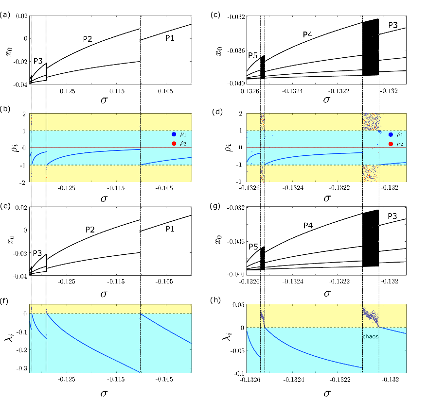
Figs. 19(b) and (d) shows the magnitude of Floquet multipliers $\rho_{1}$ and $\rho_{2}$ as the barrier distance is varied between $-0.1324\leq\sigma\leq-0.10$ and $-0.1326\leq\sigma\leq-0.1319$ . A bifurcation diagram showing amplitude response $x_{0}$ versus $\sigma$ is given for reference in Figs. 19(a) and (c). The Floquet multipliers were obtained using the higher-order saltation matrix and the TDM defined in Eqs. (30) and (34). Period-adding cascades of solutions separated by chaotic orbits were observed here with periodicity P $\#$ being defined as the number of intersections with a Poincaré section $\Sigma_{1}:x=0$ with $\ddot{x}<0$ . Results show that Floquet multipliers have a norm less than unity for the chosen $\sigma$ corresponding to a stable orbit (cyan region). As $\sigma$ is varied, the largest Floquet multiplier approaches $-1$ and becomes unstable (yellow region). This indicates that the corresponding limit cycle becomes unstable via a period-doubling bifurcation, and immediately, a new periodic orbit is observed. This is verified in the bifurcation diagram, where a DIB occurs in the same value of $\sigma$ ; see Figs. 19(a) and (c). However, the occurrence of chaotic solutions cannot be determined using Floquet multipliers, as they are applicable to dynamical systems where the Jacobian matrix is periodic. To validate the chaotic orbits observed in the amplitude response of Fig. 19(c), the largest LE (LLE) is estimated in Figs. 19(f) and (h). Results show that the LLE is always negative for $\sigma$ values with a stable periodic orbit. As $\sigma$ is varied, the LLE approaches zero, and a DIB is observed in the amplitude response. Additionally, the LLE in Fig. 19(h) is positive for a range of $\sigma$ s, implying the occurrences of chaotic orbits between period three and period four solutions; see Fig. 19(g). A comparison with the bifurcation diagram verifies the result. Therefore, the algorithms of A.1 and B.1, which implement a higher-order TDM and saltation matrix, can correctly predict bifurcation behaviour for hybrid dynamical systems. Note that there is minimal change in the computational cost when replacing the first-order with the higher-order TDM. However, the computational cost is drastically reduced when the fixed points are obtained analytically, followed by the implementation of the higher-order TDM for stability analysis Chawla and Pakrashi 2025. Further, the derivation of the proposed higher-order TDM is generalised for any $\mathbf{x}\in\mathbb{R}^{n}$ where $n\in\mathbb{Z}_{+}$ . The methodology provides a framework for identifying the governing factors and their higher-order correction terms, which significantly enhances the accuracy of post-impact state predictions in hard-impact oscillators with $n>2$ Chawla et al. 2024, Chawla et al. 2023, Chawla 2024. In particular, incorporating the higher-order flight time yields a substantial refinement over first-order approaches, such as those relying solely on saltation matrices. This methodology can be naturally extended to piecewise-smooth dynamical systems with different degrees of smoothness (DOS), such as Fillipov systems with DOS 1 or piecewise-continuous systems with DOS 2. We have developed a corresponding higher-order TDM for Filippov systems based on this same principle; the details are available in Chawla et al. 2025.

8 Conclusions

For a hybrid dynamical system of order $\mathbb{R}^{n}$ , a closed-form expression of the transverse discontinuity mapping with higher-order corrections has been derived. In addition to discrepancies near the degenerate grazing conditions, the work highlights how, even under non-degenerate conditions, the discontinuity mapping can inaccurately deduce the state of stability of the system. The proposed higher-order corrections to the time of flight presented in this paper address this issue by avoiding incorrect identification of an impact. This is deduced from the derived quadratic equation that analytically proves that not all orbits initiated in the local neighbourhood of an impacting state reach the barrier. When perturbations become too large, the discriminant of the higher-order flight time becomes negative. This indicates that perturbed orbits continue evolving in the phase-space away from the barrier. First-order transverse discontinuity mapping and the saltation matrix cannot capture this since they predict that all orbits reach the barrier. Additionally, the first-order flight time inherently possesses singularity during low-velocity impacts or grazing incidence. The higher-order correction terms resolve this limitation by ensuring that the discontinuity mappings do not diverge for low-velocity impacts.

This retention of higher order terms also improves the estimates of the mapped states of the system, which has implications for the stability of the orbit under consideration. The problem of overestimation of mapped states on the discontinuity boundary while using the first-order saltation matrix is addressed. The proposed correction terms incorporate system parameters and the functional form of the driving force of the hybrid system under consideration, leading to much closer estimates to numerical simulations. This explicit dependence on crucial parameters like the driving force is absent in a linearized approximation. The proposed approach is demonstrated using two examples of hybrid impacting systems, with single and multiple impacting barriers, respectively. It is shown that the semi-analytically obtained higher-order saltation matrix, derived with the variational approach, is able to better predict the states of the orbits post saltations, as well as provide more accurate stability estimates. The algorithm used to compute stability estimates using higher-order TDM to evaluate the LE spectra, along with its implementation method for the above examples, is provided. The analysis does not require any prior knowledge of the dynamical states at the instances of impact, unlike the approaches used for transcendental maps.

The results from this work are directly applicable to the study of complex higher periodic or aperiodic orbits in hybrid systems of order $\mathbb{R}^{n}$ , where analytically accurate estimates for trajectories interacting with the discontinuity boundary and quantification of stability are obtained, especially near bifurcation regimes when one of the attractors loses stability and/or new stable states are born.

Declarations

The authors acknowledge the funding of Research Ireland 22FFP-P11457 HarMonI, along with NexSys 21/SPP/3756 and RC2302-2 MaREI, and Sustainable Energy Authority of Ireland funded RDD/604 TwinFarm, RDD/966 FlowDyn.

Conflict of interest

The authors declare that they have no conflict of interest.

Availability of data

Not applicable.

Availability of code

All implemented codes are available upon request to the corresponding author.

Appendix A Lyapunov exponents using higher-order transverse discontinuity mapping

For a dynamical system of order $\mathbb{R}^{n}$ , the exponential divergence along the $i^{th}$ orthogonal eigenvector can be found using,

\lambda_{i}=\dfrac{1}{\tau N}\Sigma_{n=1}^{N}\log{\Big(\dfrac{r_{n}}{r_{0}}\Big)}.

(35)

The $i^{th}$ LE in Eq. (35) is evaluated by measuring the growth of the variation in the $i^{\mathrm{th}}$ direction after every time period $\tau=2\pi/\omega$ i.e., in a stroboscopic fashion. Since the state is of the order $\mathbb{R}^{n}$ , there are $n$ independent solutions of the corresponding variational form. Therefore, any arbitrary solution of the perturbed orbit can be decomposed along these $n$ eigenvectors. To measure the $i^{th}$ LE along any of these eigenvectors, a QR decomposition (QRD) is carried out using the Gram-Schmidt process. The process yields $n$ orthogonal perturbed vectors, which can be encapsulated in a hypersphere of dimension $n$ . The growth or decay of this hypersphere along the trajectory over time is an indicator of the stability of the dynamical system. The LE along an eigendirection is calculated by numerically integrating each of these orthogonal vectors and measuring the change in magnitude of these vectors after a time interval of $\tau$ where $r_{0}$ and $r_{n}$ in Eq. (35) are the initial and final magnitudes of the perturbed vector after elapsed time $\tau$ . However, for chaotic systems, the perturbed vectors might quickly diverge from the actual trajectory, and the linearized variational form might not be able to capture the actual dynamics of the perturbed trajectory. Therefore, the initial perturbed hypersphere is kept small by using a scaling factor $r_{0}$ in Eq. (35). Furthermore, to obtain accurate values of LE, $\lambda_{i}$ in Eq. (35) has been averaged out over several computations. The algorithm for estimating LEs by incorporating a higher-order TDM is presented in Algorithm A.1.

Algorithm A.1 Lyapunov exponent for hybrid systems using TDM

1. Initialize:

\mathbf{x}(0)

ensuring

H(\mathbf{x}\geq 0)

and

\omega

\alpha

\triangleright

Bifurcation parameter

2. Initialize:

\mathbf{y}_{i}(0)

for

i\leq n

using QRD

3. Rescale:

\mathbf{y}_{i}(0)\leftarrow r_{0}\times\mathbf{y}_{i}(0)

and set

n_{max}

\triangleright

Maximum allowable impacts

while count

\leq n_{max}

Integrate:

\dot{\mathbf{x}}=\mathbf{F}(\mathbf{x})

H(\mathbf{x})=0

then

\triangleright

Occurrence of impact

Evaluate:

\delta^{\xi}_{+}

\mathbf{R}(\mathbf{x})

and

\mathbf{y}_{+}

Apply reset maps:

\mathbf{x}\leftarrow\mathbf{R}(\mathbf{x})

and

\mathbf{y}_{i}\leftarrow\mathbf{y}_{i,+}

\triangleright

Implement

\mathcal{O}(2)

TDM

end if

\big(t\%\dfrac{2\pi}{\omega}\big)=0

then

if count

\geq n_{max}/2

then

Store:

r_{i}\leftarrow\dfrac{1}{r_{0}}\|\mathbf{y}_{i}\|

\triangleright

store the growth rate

end if

Reinitialize:

\mathbf{y}_{i}\leftarrow r_{0}\times\text{QRD of }\mathbf{y}_{i}

end if

end while

4: Evaluate:

\log_{e}r_{i}

\triangleright

Store all

log_{e}r_{i}

5: LE

{}_{i}\leftarrow\dfrac{\omega}{2\pi}\times\text{Partial sum of }\log_{e}r_{i}

\lambda_{i}\leftarrow\langle\text{LE}_{i}\rangle

\triangleright

Mean of all LEs

Appendix B Floquet multipliers using numerically obtained higher-order saltation matrix

Floquet theory Floquet 1883 dictates that eigenvalues of the monodromy matrix determine the stability of a limit cycle. The eigenvalues or characteristic multipliers Nayfeh and Balachandran 2008 determine the behaviour of orbits in the local linear neighbourhood of steady states. However, for hybrid dynamical systems, the monodromy matrix cannot be directly evaluated by integrating the variational equation with initial conditions corresponding to an orthogonal basis. This is due to discontinuities occurring in the state space near the discontinuity boundary. The higher-order saltation matrix is rectified by defining a state transition between the discrete mappings. Algorithm B.1 outlines the method to evaluate the Floquet multipliers using numerically obtained saltation matrices comprising higher-order correction terms.

Algorithm B.1 Floquet multipliers from monodromy matrix

\mathbf{\Phi}

1. Initialize:

\mathbf{x}(0)

ensuring

H(\mathbf{x})\geq 0

and

\omega

\alpha

\triangleright

Bifurcation parameter

2. Initialize:

\mathbf{\Phi}=\textit{I}_{n\times n}

, T

=100

, count

=0

n_{max}

\triangleright

Maximum allowable impacts

while count

\leq

n_{max}

Integrate:

\dot{\mathbf{x}}=\mathbf{F}(\mathbf{x})

H(\mathbf{x})=0

then

\triangleright

Occurrence of impact

Reset Map:

\mathbf{x}\leftarrow\mathbf{R}(\mathbf{x})

end if

\dot{x}=0

\&\&

count

\geq n_{max}/2

then

T=\{t\in\mathbb{R}^{1}:x(t+\tilde{n}T)=x(t),\tilde{n}\in\mathbb{I}\}

\triangleright

Store

x

t

for evaluation of time period

T

end if

if count

=

n_{max}

- 100 then

\triangleright

Remove transients

Store:

\mathbf{x}_{init}

\leftarrow\mathbf{x}(t)

and

t_{init}\leftarrow t

end if

end while

Initialize:

\mathbf{x}\leftarrow\mathbf{x}_{init}

t_{init}

\triangleright

Begin at steady state

Initialize:

r_{0}\ll 1

\mathbf{Y}_{1}(0)=r_{0}\textit{I}_{n\times n}

\mathbf{Y}_{2}(0)=\textit{I}_{n\times n}

\triangleright

Evaluation of

\mathbf{S}_{2}

and

\mathbf{\Phi}_{i}

while

t_{init}\leq t\leq(t_{init}+T)

\triangleright

Integrate over period

T

Integrate:

\dot{\mathbf{x}}=\mathbf{F}(\mathbf{x})

\dot{\mathbf{Y}_{1}}=(\nabla\mathbf{F})^{T}\cdot\mathbf{Y}_{1}

and

\dot{\mathbf{Y}_{2}}=(\nabla\mathbf{F})^{T}\cdot\mathbf{Y}_{2}

H(\mathbf{x})=0

then

\triangleright

Occurrence of impact

\mathbf{\Phi}_{i}\leftarrow\mathbf{Y}_{2}

and

\mathbf{\Phi}\leftarrow\mathbf{\Phi}_{i}\cdot\mathbf{\Phi}

Evaluate

\delta

and

\mathbf{y}_{+}

from

\mathbf{x}_{4}

for all

\mathbf{y}_{i}

\triangleright

TDM

Evaluate

\mathbf{Y}_{+,impact}

from

\mathbf{y}_{+}

and

\mathbf{Y}_{-\text{, impact}}\leftarrow\mathbf{Y}_{1}

Evaluate

\mathbf{S}_{2}\leftarrow\mathbf{Y}_{+,impact}\cdot\mathbf{Y}_{-,impact}^{-1}

and set

\mathbf{\Phi}\leftarrow\mathbf{S}_{2}\cdot\mathbf{\Phi}

\triangleright

saltation matrix

Reset Map:

\mathbf{x}\leftarrow\mathbf{R}(\mathbf{x})

Reinitialize:

\mathbf{Y}_{1}\leftarrow r_{0}\textit{I}_{n\times n}

and

\mathbf{Y}_{2}\leftarrow\textit{I}_{n\times n}

end if

end while

\mathbf{\Phi}\leftarrow\mathbf{Y}_{2}\cdot\mathbf{\Phi}

\triangleright

Evaluate monodromy matrix

4. Evaluate eigenvalues of

\mathbf{\Phi}

to get Floquet multipliers

References

Kahraman and Singh [1990] A. Kahraman, R. Singh, Non-linear dynamics of a spur gear pair, Journal of Sound and Vibration 142 (1990) 49–75. doi:https://doi.org/10.1016/0022-460X(90)90582-K.
Karagiannis and Pfeiffer [1991] K. Karagiannis, F. Pfeiffer, Theoretical and experimental investigations of gear-rattling, Nonlinear dynamics 2 (1991) 367–387. doi:https://doi.org/10.1007/BF00045670.
Hendriks [1983] F. Hendriks, Bounce and chaotic motion in impact print hammers, IBM Journal of Research and Development 27 (1983) 273–280. doi:https://doi.org/10.1147/rd.273.0273.
Tung and Shaw [1988] P. Tung, S. Shaw, A method for the improvement of impact printer performance (1988). doi:https://doi.org/10.1115/1.3269561.
Holmes et al. [2006] P. Holmes, R. J. Full, D. Koditschek, J. Guckenheimer, The dynamics of legged locomotion: Models, analyses, and challenges, SIAM review 48 (2006) 207–304. doi:https://doi.org/10.1137/S0036144504445133.
Goyder and Teh [1989] H. Goyder, C. Teh, A study of the impact dynamics of loosely supported heat exchanger tubes (1989). doi:https://doi.org/10.1115/1.3265696.
Païdoussis and Li [1992] M. P. Païdoussis, G. X. Li, Cross-flow-induced chaotic vibrations of heat-exchanger tubes impacting on loose supports, Journal of Sound and Vibration 152 (1992) 305–326. doi:https://doi.org/10.1016/0022-460X(92)90363-3.
Virgin and Plaut [2009] L. Virgin, R. Plaut, Some non-smooth dynamical systems in offshore mechanics, in: Vibro-Impact Dynamics of Ocean Systems and Related Problems, Springer, 2009, pp. 259–268. doi:https://doi.org/10.1007/978-3-642-00629-6_26.
Ibrahim [2014] R. A. Ibrahim, Recent advances in vibro-impact dynamics and collision of ocean vessels, Journal of Sound and Vibration 333 (2014) 5900–5916. doi:https://doi.org/10.1016/j.jsv.2014.02.006.
Xue et al. [2023] B. Xue, Y. Mao, C. Zhang, H. Zhang, Z. Qi, Nonlinear fluid-induced vibro-impact analysis on the fatigue failure pattern of a large-scale trashrack with a reduced-order model, in: Structures, volume 49, Elsevier, 2023, pp. 467–478. doi:https://doi.org/10.1016/j.istruc.2023.01.091.
Wiercigroch and Budak [2001] M. Wiercigroch, E. Budak, Sources of nonlinearities, chatter generation and suppression in metal cutting, Philosophical Transactions of the Royal Society of London. Series A: Mathematical, Physical and Engineering Sciences 359 (2001) 663–693. doi:https://doi.org/10.1098/rsta.2000.0750.
Krivtsov and Wiercigroch [1999] A. M. Krivtsov, M. Wiercigroch, Dry friction model of percussive drilling, Meccanica 34 (1999) 425–434. doi:https://doi.org/10.1023/A:1004703819275.
Wiercigroch et al. [1999] M. Wiercigroch, R. Neilson, M. Player, Material removal rate prediction for ultrasonic drilling of hard materials using an impact oscillator approach, Physics Letters A 259 (1999) 91–96. doi:https://doi.org/10.1016/S0375-9601(99)00416-8.
Feeny [1992] B. Feeny, A nonsmooth coulomb friction oscillator, Physica D: Nonlinear Phenomena 59 (1992) 25–38. doi:https://doi.org/10.1016/0167-2789(92)90204-Z.
Fan et al. [2020] J. Fan, J. Cao, S. Chen, C. Dou, S. Xue, Discontinuous dynamic analysis of a class of three degrees of freedom mechanical oscillatory systems with dry friction and one-sided rigid impact, Mechanism and Machine Theory 151 (2020) 103928. doi:https://doi.org/10.1016/j.mechmachtheory.2020.103928.
Shaw and Holmes [1983a] S. W. Shaw, P. J. Holmes, A periodically forced piecewise linear oscillator, Journal of sound and vibration 90 (1983a) 129–155. doi:https://doi.org/10.1016/0022-460X(83)90407-8.
Shaw and Holmes [1983b] S. W. Shaw, P. Holmes, A periodically forced impact oscillator with large dissipation (1983b). doi:https://doi.org/10.1115/1.3167156.
Bishop [1994] S. Bishop, Impact oscillators, Philosophical Transactions of the Royal Society of London. Series A: Physical and Engineering Sciences 347 (1994) 347–351. doi:https://doi.org/10.1098/rsta.1994.0047.
Jiang and Wiercigroch [2016] H. Jiang, M. Wiercigroch, Geometrical insight into non-smooth bifurcations of a soft impact oscillator, IMA Journal of Applied Mathematics 81 (2016) 662–678. doi:https://doi.org/10.1093/imamat/hxw004.
Luo and Chen [2005] A. C. Luo, L. Chen, Periodic motions and grazing in a harmonically forced, piecewise, linear oscillator with impacts, Chaos, Solitons & Fractals 24 (2005) 567–578. doi:https://doi.org/10.1016/j.chaos.2004.09.028.
Chillingworth and Nordmark [2013] D. Chillingworth, A. B. Nordmark, Periodic orbits close to grazing for an impact oscillator, in: Recent Trends in Dynamical Systems: Proceedings of a Conference in Honor of Jürgen Scheurle, Springer, 2013, pp. 25–37. doi:https://doi.org/10.1007/978-3-0348-0451-6_2.
Whiston [1987a] G. Whiston, The vibro-impact response of a harmonically excited and preloaded one-dimensional linear oscillator, Journal of Sound and Vibration 115 (1987a) 303–319. doi:https://doi.org/10.1016/0022-460X(87)90474-3.
Whiston [1987b] G. Whiston, Global dynamics of a vibro-impacting linear oscillator, Journal of Sound and Vibration 118 (1987b) 395–424. doi:https://doi.org/10.1016/0022-460X(87)90361-0.
Foale and Bishop [1992] S. Foale, S. Bishop, Dynamical complexities of forced impacting systems, Philosophical Transactions of the Royal Society of London. Series A: Physical and Engineering Sciences 338 (1992) 547–556. doi:https://doi.org/10.1098/rsta.1992.0020.
Foale and Bishop [1994] S. Foale, S. Bishop, Bifurcations in impact oscillations, Nonlinear dynamics 6 (1994) 285–299. doi:https://doi.org/10.1007/BF00053387.
Ma et al. [2006] Y. Ma, M. Agarwal, S. Banerjee, Border collision bifurcations in a soft impact system, Physics Letters A 354 (2006) 281–287. doi:https://doi.org/10.1016/j.physleta.2006.01.025.
Bernardo et al. [2008] M. Bernardo, C. Budd, A. R. Champneys, P. Kowalczyk, Piecewise-smooth dynamical systems: theory and applications, volume 163, Springer Science & Business Media, 2008.
Awrejcewicz and Lamarque [2003] J. Awrejcewicz, C.-H. Lamarque, Bifurcation and chaos in nonsmooth mechanical systems, volume 45, World Scientific, 2003.
Belykh et al. [2023] I. Belykh, R. Kuske, M. Porfiri, D. J. Simpson, Beyond the bristol book: Advances and perspectives in non-smooth dynamics and applications, Chaos: An Interdisciplinary Journal of Nonlinear Science 33 (2023) 010402. doi:https://doi.org/10.1063/5.0138169.
Brogliato [1999] B. Brogliato, Nonsmooth impact mechanics: models, dynamics and control, volume 3, Springer, 1999. doi:https://doi.org/10.1007/978-3-319-28664-8.
Nordmark [1991] A. B. Nordmark, Non-periodic motion caused by grazing incidence in an impact oscillator, Journal of Sound and Vibration 145 (1991) 279–297. doi:https://doi.org/10.1016/0022-460X(91)90592-8.
Nordmark [1992] A. Nordmark, Effects due to low velocity impact in mechanical oscillators, International Journal of Bifurcation and Chaos 2 (1992) 597–605. doi:https://doi.org/10.1142/S0218127492000720.
Nusse and Yorke [1992] H. E. Nusse, J. A. Yorke, Border-collision bifurcations including “period two to period three” for piecewise smooth systems, Physica D: Nonlinear Phenomena 57 (1992) 39–57. doi:https://doi.org/10.1016/0167-2789(92)90087-4.
Simpson et al. [2020] D. J. Simpson, V. Avrutin, S. Banerjee, Nordmark map and the problem of large-amplitude chaos in impact oscillators, Physical Review E 102 (2020) 022211. doi:https://doi.org/10.1103/PhysRevE.102.022211.
Nordmark [1997] A. B. Nordmark, Universal limit mapping in grazing bifurcations, Physical review E 55 (1997) 266. doi:https://doi.org/10.1103/PhysRevE.55.266.
Ma et al. [2008] Y. Ma, J. Ing, S. Banerjee, M. Wiercigroch, E. Pavlovskaia, The nature of the normal form map for soft impacting systems, International Journal of Non-Linear Mechanics 43 (2008) 504–513. doi:https://doi.org/10.1016/j.ijnonlinmec.2008.04.001.
Wiercigroch and Sin [1998] M. Wiercigroch, V. Sin, Experimental study of a symmetrical piecewise base-excited oscillator (1998). doi:https://doi.org/10.1115/1.2789108.
Banerjee et al. [2009] S. Banerjee, J. Ing, E. Pavlovskaia, M. Wiercigroch, R. K. Reddy, Invisible grazings and dangerous bifurcations in impacting systems: the problem of narrow-band chaos, Physical Review E 79 (2009) 037201. doi:https://doi.org/10.1103/PhysRevE.79.037201.
Ing et al. [2006] J. Ing, E. Pavlovskaia, M. Wiercigroch, Dynamics of a nearly symmetrical piecewise linear oscillator close to grazing incidence: Modelling and experimental verification, Nonlinear Dynamics 46 (2006) 225–238. doi:https://doi.org/10.1007/s11071-006-9045-9.
Ing et al. [2008] J. Ing, E. Pavlovskaia, M. Wiercigroch, S. Banerjee, Experimental study of impact oscillator with one-sided elastic constraint, Philosophical Transactions of the Royal Society A: Mathematical, Physical and Engineering Sciences 366 (2008) 679–705. doi:https://doi.org/10.1098/rsta.2007.2122.
Ing et al. [2010] J. Ing, E. Pavlovskaia, M. Wiercigroch, S. Banerjee, Bifurcation analysis of an impact oscillator with a one-sided elastic constraint near grazing, Physica D: Nonlinear Phenomena 239 (2010) 312–321. doi:https://doi.org/10.1016/j.physd.2009.11.009.
Pavlovskaia et al. [2010] E. Pavlovskaia, J. Ing, M. Wiercigroch, S. Banerjee, Complex dynamics of bilinear oscillator close to grazing, International Journal of Bifurcation and Chaos 20 (2010) 3801–3817. doi:https://doi.org/10.1142/S0218127410028069.
Piiroinen et al. [2004] P. T. Piiroinen, L. N. Virgin, A. R. Champneys, Chaos and period-adding; experimental and numerical verification of the grazing bifurcation, Journal of Nonlinear Science 14 (2004) 383–404. doi:https://doi.org/10.1007/s00332-004-0616-y.
Oestreich et al. [1996] M. Oestreich, N. Hinrichs, K. Popp, Bifurcation and stability analysis for a non-smooth friction oscillator, Archive of Applied Mechanics 66 (1996) 301–314. doi:https://doi.org/10.1007/BF00795247.
Oestreich et al. [1997] M. Oestreich, N. Hinrichs, K. Popp, C. Budd, Analytical and experimental investigation of an impact oscillator, in: International Design Engineering Technical Conferences and Computers and Information in Engineering Conference, volume 80425, American Society of Mechanical Engineers, 1997, p. V01CT15A008. doi:https://doi.org/10.1115/DETC97/VIB-3907.
Popp et al. [1999] K. Popp, M. Oestreich, N. Hinrichs, Numerical and experimental investigation of nonsmooth mechanical systems, in: IUTAM Symposium on New Applications of Nonlinear and Chaotic Dynamics in Mechanics, Springer, 1999, pp. 293–302. doi:https://doi.org/10.1007/978-94-011-5320-1_30.
Fredriksson and Nordmark [2000] M. H. Fredriksson, A. B. Nordmark, On normal form calculations in impact oscillators, Proceedings of the Royal Society of London. Series A: Mathematical, Physical and Engineering Sciences 456 (2000) 315–329. doi:https://doi.org/10.1098/rspa.2000.0519.
Rounak and Gupta [2020] A. Rounak, S. Gupta, Bifurcations in a pre-stressed, harmonically excited, vibro-impact oscillator at subharmonic resonances, International Journal of Bifurcation and Chaos 30 (2020) 2050111. doi:https://doi.org/10.1142/S0218127420501114.
Jiang et al. [2017] H. Jiang, A. S. Chong, Y. Ueda, M. Wiercigroch, Grazing-induced bifurcations in impact oscillators with elastic and rigid constraints, International Journal of Mechanical Sciences 127 (2017) 204–214. doi:https://doi.org/10.1016/j.ijmecsci.2017.02.001.
Chin et al. [1994] W. Chin, E. Ott, H. E. Nusse, C. Grebogi, Grazing bifurcations in impact oscillators, Physical Review E 50 (1994) 4427. doi:https://doi.org/10.1103/PhysRevE.50.4427.
Di Bernardo et al. [2002] M. Di Bernardo, P. Kowalczyk, A. Nordmark, Bifurcations of dynamical systems with sliding: derivation of normal-form mappings, Physica D: Nonlinear Phenomena 170 (2002) 175–205. doi:https://doi.org/10.1016/S0167-2789(02)00547-X.
Budd and Dux [1994] C. Budd, F. Dux, Chattering and related behaviour in impact oscillators, Philosophical Transactions of the Royal Society of London. Series A: Physical and Engineering Sciences 347 (1994) 365–389. doi:https://doi.org/10.1098/rsta.1994.0049.
Thompson and Ghaffari [1983] J. Thompson, R. Ghaffari, Chaotic dynamics of an impact oscillator, Physical Review A 27 (1983) 1741. doi:https://doi.org/10.1103/PhysRevA.27.1741.
Hassouneh et al. [2004] M. A. Hassouneh, E. H. Abed, H. E. Nusse, Robust dangerous border-collision bifurcations in piecewise smooth systems, Physical review letters 92 (2004) 070201. doi:https://doi.org/10.1103/PhysRevLett.92.070201.
Chawla et al. [2024] R. Chawla, A. Rounak, C. Bose, V. Pakrashi, Wake-induced response of vibro-impacting systems, Physics of Fluids 36 (2024). doi:https://doi.org/10.1063/5.0236147.
Leine [2000] R. I. Leine, Bifurcations in discontinuous mechanical systems of the fillippov-type (2000). doi:https://doi.org/10.6100/IR533239.
Yin et al. [2018] S. Yin, G. Wen, H. Xu, X. Wu, Higher order zero time discontinuity mapping for analysis of degenerate grazing bifurcations of impacting oscillators, Journal of Sound and Vibration 437 (2018) 209–222. doi:https://doi.org/10.1016/j.jsv.2018.08.048.
Kundu et al. [2012] S. Kundu, S. Banerjee, J. Ing, E. Pavlovskaia, M. Wiercigroch, Singularities in soft-impacting systems, Physica D: Nonlinear Phenomena 241 (2012) 553–565. doi:https://doi.org/10.1016/j.physd.2011.11.014.
di Bernardo et al. [2001] M. di Bernardo, C. Budd, A. Champneys, Normal form maps for grazing bifurcations in n-dimensional piecewise-smooth dynamical systems, Physica D: Nonlinear Phenomena 160 (2001) 222–254. doi:https://doi.org/10.1016/S0167-2789(01)00349-9.
Di Bernardo et al. [2001] M. Di Bernardo, C. J. Budd, A. R. Champneys, Grazing and border-collision in piecewise-smooth systems: A unified analytical framework, Physical Review Letters 86 (2001) 2553. doi:https://doi.org/10.1103/PhysRevLett.86.2553.
Floquet [1883] G. Floquet, On linear differential equations with periodic coefficients, in: Annales scientifiques de l’École Normale Supérieure, volume 12, 1883, pp. 47–88.
Nayfeh and Balachandran [2008] A. H. Nayfeh, B. Balachandran, Applied nonlinear dynamics: analytical, computational, and experimental methods, John Wiley & Sons, 2008.
Oseledec [1968] V. I. Oseledec, A multiplicative ergodic theorem. liapunov characteristic number for dynamical systems, Trans. Moscow Math. Soc. 19 (1968) 197–231.
Pesin [1977] Y. B. Pesin, Characteristic lyapunov exponents and smooth ergodic theory, Russian Mathematical Surveys 32 (1977) 55. doi:https://doi.prg/10.1070/RM1977v032n04ABEH001639.
Benettin et al. [1980] G. Benettin, L. Galgani, A. Giorgilli, J.-M. Strelcyn, Lyapunov characteristic exponents for smooth dynamical systems and for hamiltonian systems; a method for computing all of them. part 1: Theory, Meccanica 15 (1980) 9–20. doi:https://doi.org/10.1007/BF02128236.
Bennetin et al. [1980] G. Bennetin, L. Galgani, A. Giorgilli, J.-M. Strelcyn, Lyapunov characteristic exponents for smooth dynamical systems and for hamiltonian systems: A method for computing all of them. part 2: Numerical application, Meccanica 15 (1980) 21–30. doi:https://doi.org/10.1007/BF02128236.
Lamba and Budd [1994] H. Lamba, C. Budd, Scaling of lyapunov exponents at nonsmooth bifurcations, Physical Review E 50 (1994) 84. doi:https://doi.org/10.1103/PhysRevE.50.84.
Müller [1995] P. C. Müller, Calculation of lyapunov exponents for dynamic systems with discontinuities, Chaos, Solitons & Fractals 5 (1995) 1671–1681. doi:https://doi.org/10.1016/0960-0779(94)00170-U.
De Souza and Caldas [2004] S. L. De Souza, I. L. Caldas, Calculation of lyapunov exponents in systems with impacts, Chaos, Solitons & Fractals 19 (2004) 569–579. doi:https://doi.org/10.1016/S0960-0779(03)00130-9.
Jin et al. [2006] L. Jin, Q.-S. Lu, E. Twizell, A method for calculating the spectrum of lyapunov exponents by local maps in non-smooth impact-vibrating systems, Journal of sound and Vibration 298 (2006) 1019–1033. doi:https://doi.org/10.1016/j.jsv.2006.06.035.
Leine [2012] R. Leine, Non-smooth stability analysis of the parametrically excited impact oscillator, International Journal of Non-Linear Mechanics 47 (2012) 1020–1032. doi:https://doi.org/10.1016/j.ijnonlinmec.2012.06.010.
Mandal et al. [2013] K. Mandal, C. Chakraborty, A. Abusorrah, M. Al-Hindawi, Y. Al-Turki, S. Banerjee, An automated algorithm for stability analysis of hybrid dynamical systems, The European Physical Journal Special Topics 222 (2013) 757–768. doi:https://doi.org/10.1140/epjst/e2013-01879-x.
Stefanski [2000] A. Stefanski, Estimation of the largest lyapunov exponent in systems with impacts, Chaos, Solitons & Fractals 11 (2000) 2443–2451. doi:https://doi.org/10.1016/S0960-0779(00)00029-1.
Stefanski et al. [2005] A. Stefanski, A. Dabrowski, T. Kapitaniak, Evaluation of the largest lyapunov exponent in dynamical systems with time delay, Chaos, Solitons & Fractals 23 (2005) 1651–1659. doi:https://doi.org/10.1016/j.chaos.2004.06.051.
Dabrowski [2012] A. Dabrowski, Estimation of the largest lyapunov exponent from the perturbation vector and its derivative dot product, Nonlinear Dynamics 67 (2012) 283–291. doi:https://doi.org/10.1007/s11071-011-9977-6.
Li et al. [2018] T. Li, C.-H. Lamarque, S. Seguy, A. Berlioz, Chaotic characteristic of a linear oscillator coupled with vibro-impact nonlinear energy sink, Nonlinear Dynamics 91 (2018) 2319–2330. doi:https://doi.org/10.1007/s11071-017-4015-y.
Balcerzak et al. [2020] M. Balcerzak, A. Dabrowski, B. Blazejczyk-Okolewska, A. Stefanski, Determining lyapunov exponents of non-smooth systems: Perturbation vectors approach, Mechanical Systems and Signal Processing 141 (2020) 106734. doi:https://doi.org/10.1016/j.ymssp.2020.106734.
Han et al. [1995] R. Han, A. Luo, W. Deng, Chaotic motion of a horizontal impact pair, Journal of Sound and Vibration 181 (1995) 231–250. doi:https://doi.org/10.1006/jsvi.1995.0137.
Strogatz [2018] S. H. Strogatz, Nonlinear dynamics and chaos: with applications to physics, biology, chemistry, and engineering, CRC press, 2018. doi:https://doi.org/10.1201/9780429398490.
Chawla and Pakrashi [2025] R. Chawla, V. Pakrashi, Higher-order poincaré maps for stability analysis of impact oscillators, in: Journal of Physics: Conference Series, volume 2983, IOP Publishing, 2025, p. 012002. doi:https://doi.org/10.1088/1742-6596/2983/1/012002.
Chawla et al. [2023] R. Chawla, A. Rounak, V. Pakrashi, Higher order transverse discontinuity mapping for hybrid dynamical systems, in: International Conference on Nonlinear Dynamics and Applications, Springer, 2023, pp. 677–687. doi:https://doi.org/10.1007/978-3-031-50631-4_57.
Chawla [2024] R. Chawla, Discontinuity mappings in piecewise-smooth dynamical systems, Ph.D. thesis, University College Dublin. School of Mechanical and Materials Engineering, 2024. doi:http://hdl.handle.net/10197/28846.
Chawla et al. [2025] R. Chawla, S. Seth, A. Rounak, V. Pakrashi, Higher-order transverse discontinuity mapping in filippov systems: Analysis and experimental validation using an electronic circuit, arXiv preprint arXiv:2506.18379 (2025). doi:https://doi.org/10.48550/arXiv.2506.18379.