A Measurement of the Effective Mean-Free-Path of Solar Wind ProtonsPreprint: APS/123-QED

Introduction.— Many natural plasmas (e.g., interstellar medium, galaxy clusters, black hole accretion disks, solar wind) are in a weakly collisional state, where the particle collision frequency $\nu_{\mathrm{coll}}$ is smaller than other characteristic frequencies (e.g., proton gyrofrequency $\Omega_{\mathrm{p}}$, inverse magnetic field correlation time $1/\tau_{c}$ etc.) (Schekochihin et al. 2009; Marsch 2006; Schekochihin and Cowley 2006; Quataert 2003). Thus, the characteristic timescales of the plasma motions $\omega$ can span from collisional (fluid) $\omega\ll\nu_{\mathrm{coll}}$ to collisionless $\omega\gg\nu_{\mathrm{coll}}$ (Schekochihin et al. 2009; Schekochihin et al. 2005). Knowledge of the transition scale $\omega\sim\nu_{\mathrm{coll}}$ is vital to understand the thermodynamics of astrophysical plasmas (Schekochihin et al. 2009).

The escaping solar corona, known as the solar wind, expands into interplanetary space as a super-Alfvénic and turbulent plasma (Parker 1958; Bruno and Carbone 2013; Verscharen et al. 2019). In situ measurements of particle distribution functions and electromagnetic fields enable fundamental plasma physics observations (Chen 2016). The Spitzer-Härm proton-proton collision frequency $\nu_{\mathrm{p},\mathrm{p}}^{\mathrm{SH}}$ decreases with radial distance from the Sun, and by a few solar radii, is much smaller than other characteristic frequencies. In principle, the dynamics should be described by collisionless plasma equations. For reference, at 1 AU, typical frequencies are $\nu_{\mathrm{p},\mathrm{p}}^{\mathrm{SH}}\approx 4\times 10^{-7}\,\mathrm{s}^{-1}$, $\Omega_{\mathrm{p}}\approx 10^{-1}\,\mathrm{s}^{-1}$, $1/\tau_{c}\approx 10^{-6}\,\mathrm{s}^{-1}$  (Book 1987; Spitzer 2006; Verscharen et al. 2019; Matthaeus et al. 2010).

Despite the weak collisionality of the solar wind, many aspects appear to be described by fluid equations: magnetohydrodynamic (MHD) turbulence theory predicts the shape of power spectra (e.g., magnetic field, proton density) (Coleman 1968; Matthaeus and Goldstein 1982; Bruno and Carbone 2013; Goldreich and Sridhar 1997; Tu and Marsch 1995), spatial transport (Matthaeus et al. 1999; Zank et al. 1996), and the proton heating rate by the energy cascade (MacBride et al. 2008; Stawarz et al. 2009; Coburn et al. 2012). While this is due, in part, to the dominance of Alfvénic fluctuations (Schekochihin et al. 2009; Lithwick and Goldreich 2001; Howes et al. 2008; Quataert 1998), compressive fluctuations, that should be severely damped in a collisionless plasma (Barnes 1966), display the MHD slow-mode polarization (magnetic and thermal pressure anticorrelated). They are routinely detected at a range of scales (Tu and Marsch 1995; Howes et al. 2012; Klein et al. 2012; Kellogg and Horbury 2005; Yao et al. 2013a; Yao et al. 2013b; Yao et al. 2011) following a power law predicted from the MHD equations (Montgomery et al. 1987; Schekochihin et al. 2009; Lithwick and Goldreich 2001; Marsch and Tu 1990a). The most clear evidence of fluid behavior can be seen in the strong correlation between the density and thermal pressure, indicating a polytropic equation of state (Marsch et al. 1983; Nicolaou et al. 2020; Totten et al. 1995; Verscharen et al. 2017).

While the Spitzer-Härm collision frequency appears incompatible with the fluidlike behavior of the solar wind, weakly collisional plasmas are also subject to nonlinear processes that prevent extreme departure from equilibrium (Nishida 1969; Griffel and Davis 1969; Yoon 2017; Hamasaki and Krall 1973; Gary et al. 2000). Solar wind observations present substantial evidence of temperature anisotropy instabilities constraining the particle distribution functions (Kasper et al. 2002; Hellinger et al. 2006; Chen et al. 2016; Marsch 2006; Tu and Marsch 2002; Yoon 2017) suggesting they experience pitch-angle scattering by plasma waves (Bale et al. 2009). These processes can play a similar role to collisions i.e., they are effective collision processes.

This Letter presents a measurement of the effective mean-free-path of the solar wind by comparing observations of compressive wave-mode polarizations to numerical solutions of varying effective collisionality. It is shown that the transition from fluid to collisionless dynamics in the solar wind occurs at scales several orders of magnitude below the classical Spitzer-Härm mean-free-path, explaining the fluidlike behavior of the weakly collisional solar wind.

Theory and numerical solutions.— The kinetic MHD equations with the Bhatnagar-Gross-Krook (BGK) collision operator (Bhatnagar et al. 1954; Gross and Krook 1956) produce dispersion relations and plasma fluctuations (e.g., magnetic field and pressure) that span between the collisionless and collisional limits (Snyder et al. 1997; Sharma et al. 2003; Kulsrud et al. 1980). They describe a nonrelativistic, magnetized plasma of arbitrary collision frequency (Kulsrud et al. 1980; Sharma et al. 2003). The specific equations, which we refer to as KMHD-BGK, model both the proton and electron responses with the kinetic equation. The BGK operator is used here to model relaxation processes, not particle collisions, so we use the language of an effective proton collision frequency $\nu_{\mathrm{eff}}$ or mean-free-path $\lambda_{\mathrm{mfp}}^{\text{eff}}=v_{\text{th}}^{\mathrm{p}}/\nu_{\mathrm{eff}}$, where the proton thermal speed is $v_{\text{th}}^{\mathrm{p}}$ (see Supplemental Material).

Assuming plasma motions are slow compared to the gyrofrequency $\Omega_{p}$, the second moment of the kinetic equation and the ideal induction equation leads to,

where $d/dt$ is the convective derivative and the quantities are the proton density $n_{\mathrm{p}}$, magnetic-field strength $B$, (perpendicular) parallel $(p_{\perp}^{\mathrm{p}})\;p_{\parallel}^{\mathrm{p}}$ proton pressure, field parallel flux of (perpendicular) parallel $(q_{\perp}^{\mathrm{p}})\;q_{\parallel}^{\mathrm{p}}$ proton heat, and the unit magnetic field vector $\hat{\bm{b}}=\bm{B}/B$ (Chew et al. 1956; Hunana et al. 2019). The Alfvén speed is $v_{A}=B/\sqrt{4\pi n_{\mathrm{p}}m_{\mathrm{p}}}$, the proton gyroradius is $\rho_{\mathrm{p}}=v_{\mathrm{th}}^{\mathrm{p}}/\Omega_{\mathrm{p}}$, and the ion-acoustic speed is $c_{\mathrm{s}}=\sqrt{(3k_{\mathrm{B}}T_{\parallel}^{\mathrm{p}}+k_{\mathrm{B}}T_{\parallel}^{\mathrm{e}})/m_{\mathrm{p}}}$, where the parallel proton (electron) temperature is $T_{\parallel}^{\mathrm{p}}\;(T_{\parallel}^{\mathrm{e}})$.

Equations (1) are often discussed when the right hand sides are zero and are then referred to as the double adiabatic equations or Chew-Goldberger-Low (CGL) invariants (Chew et al. 1956). The focus here is on how the CGL invariants are broken, for example, by the heat flux terms in the collisionless limit, and by the collisional terms ($\propto\nu_{\mathrm{eff}}$). Therefore, the relative conservation of the CGL invariants provides a sensitive test of the equation of state (Schekochihin et al. 2010).

We proceed by constructing measures that describe the correlation and amplitude ratios of the left hand sides of Eqs. (1),

where $\delta\chi=\chi-\langle\chi\rangle$ is the fluctuation about the average $\langle\chi\rangle$. The method compares predictions for Eqs. (2) derived from the slow-mode eigenmodes of the linearized KMHD-BGK system (e.g., $\delta p_{\perp}^{\mathrm{p}},\,\delta B$ etc.) to solar wind measurements. See Supplemental Material.

The model’s free parameters are the propagation angle $\theta_{\hat{\bm{b}},\hat{\bm{k}}}$ and proton effective mean-free-path $\lambda_{\mathrm{mfp}}^{\mathrm{eff}}$, i.e., they can be measured. The wavenumber $k$ and the proton beta $\beta=8\pi k_{B}p^{\mathrm{p}}/B^{2}$ where $p^{\mathrm{p}}=2p^{\mathrm{p}}_{\perp}/3+p^{\mathrm{p}}_{\parallel}/3$ are set to measured values. The species temperature ratio is set to a typical value for the solar wind $T_{\mathrm{p}}/T_{\mathrm{e}}=1$ and the effective mean-free-path species ratio is set to $\lambda_{\mathrm{mfp}}^{\mathrm{eff}}/\lambda_{\mathrm{mfp,electrons}}^{\mathrm{eff}}=5$; see Supplemental Material at for details of electron physics.

The top panels of Fig. 1 demonstrate the ability of the KMHD-BGK equations to resolve the dynamics of the compressive slow-mode from collisional (lighter blue) to collisionless (black) (Sharma et al. 2003). Numerical predictions for Eqs. (2a), (2c) (bottom panels of Fig. 1) show distinct differences at $\beta>1$ for $k_{\parallel}\lambda_{\mathrm{mfp}}^{\mathrm{eff}}$, which can be compared to observations. The MHD/collisionless limits are illustrated in magenta, for $C_{\perp}$ (bottom right panel) these two limits produce similar trends, therefore it is necessary to make comparisons at multiple $k_{\parallel}$, to measure $\lambda_{\mathrm{mfp}}^{\mathrm{eff}}$.

Measurements.— The dataset consists of Wind spacecraft measurements of the pristine solar wind during years 2005-2010. The electrostatic analyzer 3DP records onboard moments of the proton density, velocity and pressure tensor, and the magnetometer MFI records the magnetic field, at a nominal $\sim 3s$ cadence (Lin et al. 1995; Lepping et al. 1995).

The dataset is restricted to time intervals satisfying three criteria: (i) 95% of the data is available (the remaining is then linearly interpolated); (ii) the median density must be greater than 1 particle per cm^-3; and (iii) the average norm of the non-gyrotropic tensor ($\mathsf{\Pi}^{\mathrm{p}}=\mathsf{p}^{\mathrm{p}}-\hat{\bm{b}}\hat{\bm{b}}\,p^{\mathrm{p}}_{\parallel}-(\mathsf{1}-\hat{\bm{b}}\hat{\bm{b}})p_{\perp}^{\mathrm{p}}$), must be less than 30% of the average norm of the pressure tensor $\mathsf{p}^{\mathrm{p}}$.

To probe a set of wavenumbers we measure the four quantities in Eqs. (2), the average radial solar wind velocity $\langle V_{\mathrm{SW}}\rangle$, and average proton beta for a set of time intervals $\tau=[30\text{s},\,1\text{min.},\,2\text{mins.},\,...,\,128\text{mins.}]$. The time scales are converted to wavenumber $k_{\mathrm{SW}}=1/\tau\langle V_{\mathrm{SW}}\rangle$ via Taylor’s frozen-in-flow (TFF) assumption (Taylor 1938). Three bins of equal probability density are obtained where the median of each bin is $k_{\mathrm{SW}}=[0.288,1.41,6.34]\times 10^{-5}\,\mathrm{km}^{-1}$, which lie within the inertial range of the magnetic field power spectrum at 1 AU (Kiyani et al. 2015). The wavenumber bins contain $[2.98,16.6,70.0]\times 10^{5}$ samples.

For bin $k_{\mathrm{SW}}=0.288\times 10^{-5}\,\mathrm{km}^{-1}$ the $\beta$-conditioned probability functions of Eqs. (2), all mapped to a common color bar, are displayed in Fig. 2. The $\beta$-trend lines in magenta (see caption) capture statistically significant differences between $\beta\lessgtr 1$. From the correlations $C_{\parallel},C_{\perp}$ it is clear that the CGL invariants are rarely conserved $(C_{\parallel},C_{\perp}=1)$, but display similar trends to the theoretical expectations (Fig. 1). The amplitude ratios $A_{\parallel},A_{\perp}$ demonstrate a relative decrease in fluctuation amplitude of the pressure components at $\beta>1$.

Comparison of measurements and numerical solutions.— To compare theoretical predictions of Eqs. 2 to observations, a degeneracy in parametrization must be dealt with: the numerical solutions primarily depend on $k_{\parallel}\lambda_{\mathrm{mfp}}^{\mathrm{eff}}=k\,\mathrm{cos}\big(\theta_{\hat{\bm{b}},\hat{\bm{k}}}\big)\lambda_{\mathrm{mfp}}^{\mathrm{eff}}$ (Sharma et al. 2003); such that $\lambda_{\mathrm{mfp}}^{\mathrm{eff}},\,\theta_{\hat{\bm{b}},\hat{\bm{k}}}$ are degenerate. To address this we introduce a scale dependent anisotropy model $(k_{\parallel}\sim k_{\perp}^{\alpha})$, which relates $k$ and $\theta_{\hat{\bm{b}},\hat{\bm{k}}}$,

where $k_{\mathrm{iso}}$ is the isotropic wavenumber ($k_{\perp}=k_{\parallel}$) and $\alpha$ is the anisotropy exponent, generalised from turbulence models (Goldreich and Sridhar 1995). Comparing solutions parameterized by $\lambda_{\mathrm{mfp}}^{\mathrm{eff}},\,\alpha,\,k_{\mathrm{iso}}$ across multiple wavenumbers $k=k_{\mathrm{SW}}$ clears the degeneracy.

Finally, the predictions of Eqs. (2) from the numerical solutions are normalized to the measured $\beta$-conditioned mean value (dashed magenta lines in Fig. 2) of $C_{\parallel},C_{\perp},A_{\parallel},A_{\perp}$ at $\beta\simeq 10^{-1}$. This is to account for the fact that linear polarizations are only approximately observed in strong turbulence (Chen 2016).

Ranges of $\alpha,\,k_{\mathrm{iso}},\,\lambda_{\mathrm{mfp}}^{\mathrm{eff}}=[0.05,1.0],\,[5\times 10^{-9},5\times 10^{-7}]\,\mathrm{km}^{-1},\,[3.5\times 10^{4},2.1\times 10^{6}]\,\mathrm{km}$ are chosen for computing numerical solutions. The ranges of $\alpha,k_{\mathrm{iso}}$ are consistent with previous observations (Chen et al. 2012; Chen 2016). The range of $\lambda_{\mathrm{mfp}}^{\mathrm{eff}}$ returns numerical solutions of Eqs. (2) that compare qualitatively well with the observations (seen in Fig. 2). The Spitzer-Härm mean-free-path returns the (collisionless) ion-acoustic dispersion relation which is inconsistent with the measurements.

To make a quantitative comparison, we compute the “goodness of fit”,

where $\hat{y}_{i}$ ($\bar{y}_{i}$) is the local numerical solution (local measured mean), summed over $i$, denoting the $i$th $\beta$-bin. $R(k_{\mathrm{SW}};\alpha,k_{\mathrm{iso}},\lambda_{\mathrm{mfp}}^{\mathrm{eff}})$ is calculated for each wavenumber $k_{\mathrm{SW}}$, where the mean $\bar{y}_{i}$ is respective to the wavenumber bin. The $R$-values are inverted for unnormalized weights ($w=R^{-1}$), divided by the maximum weight, then summed over wavenumber $\mathcal{W}=\sum_{k}w(k;\alpha,k_{\mathrm{iso}},\lambda_{\mathrm{mfp}}^{\mathrm{eff}})$ to break the aforementioned degeneracy. From this volume, weighted geometric means $\mu_{x}$, covariances $\sigma^{2}_{x,y}$, and two sigma confidence intervals $\mathrm{CI}_{x}$ are calculated (see Supplemental Material) (Kendall and Stuart 1977; Norris 1940). This is the method we employ to measure the quantities $\lambda_{\mathrm{mfp}}^{\mathrm{eff}},\alpha,k_{\mathrm{iso}}$, providing the main results of the Letter.

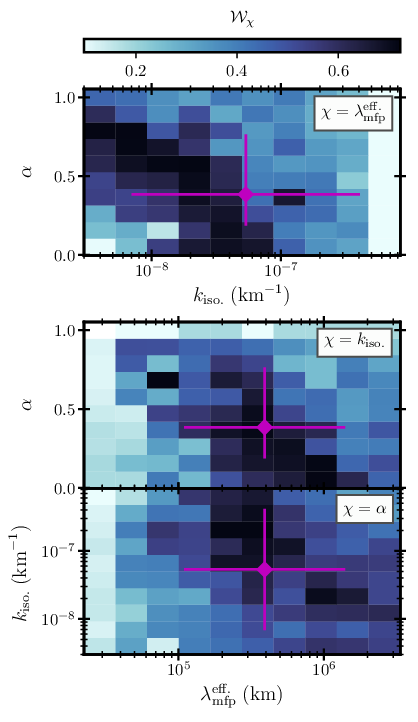
To visualize the weighted parameter space for $C_{\perp}$, Fig. 3 illustrates the weight volume $\mathcal{W}(\alpha,k_{\mathrm{iso}},\lambda_{\mathrm{mfp}}^{\mathrm{eff}})$, numerically integrated over each parameter axis $\chi$,

where $\chi_{n},\chi_{0}$ are limits of the range. The weighted means in Fig. 3 lie in the maximum regions of $\mathcal{W}_{\chi}$, within the confidence intervals, indicating the weighted geometric statistics are a good representation of the observations.

To check the scale dependence, Fig. 4 displays the observed $\beta$-conditioned means of Eqs. (2) and the numerical solutions corresponding to the maximum $\mathcal{W}$. The numerical solutions and observations trend similarly with wavenumber indicating the scale dependence of the effective collisionality has been well modeled. The parameters of the maxima (recorded in the panels of Fig. 4) do not correspond exactly to the weighted geometric means of $\mathcal{W}$ (seen in Fig. 3) reflecting the statistical nature of the measured quantities.

The method of calculating statistics for $\lambda_{\mathrm{mfp}}^{\mathrm{eff}},\,\alpha,\,k_{\mathrm{iso}}$ displayed in Fig. 3 for $C_{\perp}$ produces similar statistics for $C_{\parallel},A_{\parallel},A_{\perp}$ (see Supplemental Material). Therefore, in Table 1 combined statistics are reported. The measured effective mean-free-path and mean proton thermal speed (measured with this data set) gives an effective collision frequency of $\nu_{\mathrm{eff}}=v_{\mathrm{th}}^{\mathrm{p}}/\lambda_{\mathrm{mfp}}^{\mathrm{eff}}$ = 1.11 $\times 10^{-4}$ s^-1.

The transition frequency, where $\nu_{\mathrm{eff}}\simeq\omega$ can be estimated with $\nu_{\mathrm{eff}}=v_{\mathrm{th}}^{\mathrm{p}}/\lambda_{\mathrm{mfp}}^{\mathrm{eff}}$ and the ion-acoustic dispersion relation $\omega_{\mathrm{IA}}=k_{\parallel}\,c_{\mathrm{s}}$, giving the parallel transition wavenumber $k^{\mathrm{trans}}_{\parallel}=v_{\mathrm{th}}^{\mathrm{p}}/c_{\mathrm{s}}\,\lambda_{\mathrm{mfp}}^{\mathrm{eff}}$ (Sharma et al. 2003; Verscharen et al. 2017; Kunz et al. 2020). Using the wavenumber model (Eq. (3)), the transition wavenumber is,

Inserting the combined statistics from Table 1, using a typical value of $v_{\mathrm{th}}^{\mathrm{p}}/c_{\mathrm{s}}=\sqrt{1/2}$ for the solar wind, and using the TFF assumption, the transition wavenumber in spacecraft-frame frequency at 1 AU is $\langle V_{\mathrm{SW}}\rangle\,k^{\mathrm{trans}}=f^{\mathrm{trans}}=0.19$ Hz, and $\mathrm{CI}_{f^{\mathrm{trans}}}=[0.046,\,0.33]$ Hz. The uncertainties are propagated from $V_{\mathrm{SW}}$ and the four estimates of $k^{\mathrm{trans}}$ from $C_{\parallel},\,A_{\parallel},\,C_{\perp},\,A_{\perp}$.

Discussion.— We have measured the relative non-conservation of the CGL invariants and modeled the behavior with the slow-mode branch of the KMHD-BGK equations to measure the effective mean-free-path of the solar wind protons and the scale dependence of the slow-mode wavenumber anisotropy (Table 1 reports the statistics of these measurements). The primary result of this Letter is the measured effective proton mean-free-path that is $\sim 10^{3}$ times smaller than the Spitzer-Härm mean-free-path ($\lambda_{\mathrm{mfp}}^{\mathrm{SH}}=1.14\times 10^{8}\,\mathrm{km}$, measured with this dataset). Therefore, the fluidlike range in the solar wind extends to much smaller scales than predicted based on particle collisions. In addition, the scale dependent anisotropy of the compressive fluctuations ($\alpha\simeq 0.4$) is consistent with previous measurements (Chen et al. 2012; Chen 2016), being more anisotropic than the Alfvénic fluctuations.

The measured transition frequency, the scale between fluid behavior ($f\ll f^{\mathrm{trans}}$) and collisionless behavior ($f\gg f^{\mathrm{trans}}$), of $f^{\mathrm{trans}}=0.189$ Hz is at the well-known break in power law $(k_{\perp}\rho_{\mathrm{p}}\sim 1)$ of the magnetic field power spectrum at 1 AU (Leamon et al. 1998; Kiyani et al. 2015; Verscharen et al. 2019). These measurements therefore justify the use of fluid MHD theory at larger scales $(k_{\perp}\rho_{\mathrm{p}}<1)$ (Zank et al. 1996; Matthaeus and Goldstein 1982; Chen 2016; Montgomery et al. 1987; Tu and Marsch 1995; Coleman 1968; Bruno and Carbone 2013; Goldreich and Sridhar 1997; Matthaeus et al. 1999; Stawarz et al. 2009; Coburn et al. 2012; MacBride et al. 2008; Marsch and Tu 1990b). If the result $k_{\perp}\rho_{\mathrm{p}}\simeq k_{\parallel}\lambda^{\mathrm{eff}}_{\mathrm{mfp}}$ turns out to be a general property of weakly collisional plasma, this provides a simple parameterization for the effective collisionality of astrophysical plasmas.

Effective collisional processes have long been studied theoretically and numerically (Schekochihin and Cowley 2006; Rincon et al. 2016; Helander et al. 2016; Kunz et al. 2016; Squire et al. 2017; Kunz et al. 2014; Coroniti and Eviatar 1977), but it is an open question as to the relevant role of the various mechanisms (Gary et al. 2000; Hamasaki and Krall 1973; Marsch 2006; Yoon 2017; Meyrand et al. 2019; Schekochihin et al. 2016; Kellogg 2000)) and how they are activated (Squire et al. 2017; Kunz et al. 2020; Verscharen et al. 2016). Therefore, further studies are necessary to assess exactly what key physics of weakly collisional plasma leads to the measured effective collisionality, since most astrophysical plasmas, being multi-scale and turbulent, will support effective collision mechanisms (Zhuravleva et al. 2019). The measurements presented here provide constraints to be satisfied by theories of effective collision processes.

Supplemental Materials: Title for main text

References

- Schekochihin et al. (2009) A. A. Schekochihin, S. C. Cowley, W. Dorland, G. W. Hammett, G. G. Howes, E. Quataert, and T. Tatsuno, Astrophys. J., Suppl. Ser. 182, 310 (2009).
- Marsch (2006) E. Marsch, Living Rev. Sol. Phys. 3, 1 (2006).
- Schekochihin and Cowley (2006) A. A. Schekochihin and S. C. Cowley, Phys. Plasmas 13, 056501 (2006).
- Quataert (2003) E. Quataert, Astron. Nachr. 324, 435 (2003).
- Schekochihin et al. (2005) A. A. Schekochihin, S. C. Cowley, R. M. Kulsrud, G. W. Hammett, and P. Sharma, Astrophys. J. 629, 139 (2005).
- Parker (1958) E. N. Parker, Astrophys. J. 128, 664 (1958).
- Bruno and Carbone (2013) R. Bruno and V. Carbone, Living Rev. Sol. Phys. 10, 2 (2013).
- Verscharen et al. (2019) D. Verscharen, K. G. Klein, and B. A. Maruca, Living Rev. Sol. Phys. 16, 5 (2019).
- Chen (2016) C. H. K. Chen, J. Plasma Phys. 82, 535820602 (2016).
- Book (1987) D. L. Book, NRL (Naval Research Laboratory) Plasma Formulary. Revised., Tech. Rep. (NAVAL RESEARCH LAB WASHINGTON DC, 1987).
- Spitzer (2006) L. Spitzer, Physics of fully ionized gases (Courier Corporation, 2006).
- Matthaeus et al. (2010) W. H. Matthaeus, S. Dasso, J. M. Weygand, M. G. Kivelson, and K. T. Osman, Astrophys. J., Lett. 721, L10 (2010).
- Coleman (1968) J. Coleman, Paul J., Astrophys. J. 153, 371 (1968).
- Matthaeus and Goldstein (1982) W. H. Matthaeus and M. L. Goldstein, J. Geophys. Res. 87, 6011 (1982).
- Goldreich and Sridhar (1997) P. Goldreich and S. Sridhar, Astrophys. J. 485, 680 (1997).
- Tu and Marsch (1995) C.-Y. Tu and E. Marsch, Space Sci. Rev. 73, 1 (1995).
- Matthaeus et al. (1999) W. H. Matthaeus, G. P. Zank, C. W. Smith, and S. Oughton, Phys. Rev. Lett. 82, 3444 (1999).
- Zank et al. (1996) G. P. Zank, W. H. Matthaeus, and C. W. Smith, J. Geophys. Res. 101, 17093 (1996).
- MacBride et al. (2008) B. T. MacBride, C. W. Smith, and M. A. Forman, Astrophys. J. 679, 1644 (2008).
- Stawarz et al. (2009) J. E. Stawarz, C. W. Smith, B. J. Vasquez, M. A. Forman, and B. T. MacBride, Astrophys. J. 697, 1119 (2009).
- Coburn et al. (2012) J. T. Coburn, C. W. Smith, B. J. Vasquez, J. E. Stawarz, and M. A. Forman, Astrophys. J. 754, 93 (2012).
- Lithwick and Goldreich (2001) Y. Lithwick and P. Goldreich, Astrophys. J. 562, 279 (2001).
- Howes et al. (2008) G. G. Howes, S. C. Cowley, W. Dorland, G. W. Hammett, E. Quataert, and A. A. Schekochihin, J. Geophys. Res., Space Phys. 113, A05103 (2008).
- Quataert (1998) E. Quataert, Astrophys. J. 500, 978 (1998).
- Barnes (1966) A. Barnes, Phys. Fluids 9, 1483 (1966).
- Howes et al. (2012) G. G. Howes, S. D. Bale, K. G. Klein, C. H. K. Chen, C. S. Salem, and J. M. TenBarge, Astrophys. J., Lett. 753, L19 (2012).
- Klein et al. (2012) K. G. Klein, G. G. Howes, J. M. TenBarge, S. D. Bale, C. H. K. Chen, and C. S. Salem, Astrophys. J. 755, 159 (2012).
- Kellogg and Horbury (2005) P. J. Kellogg and T. S. Horbury, Ann. Geophys 23, 3765 (2005).
- Yao et al. (2013a) S. Yao, J. S. He, C. Y. Tu, L. H. Wang, and E. Marsch, Astrophys. J. 776, 94 (2013a).
- Yao et al. (2013b) S. Yao, J. S. He, C. Y. Tu, L. H. Wang, and E. Marsch, Astrophys. J. 774, 59 (2013b).
- Yao et al. (2011) S. Yao, J. S. He, E. Marsch, C. Y. Tu, A. Pedersen, H. Rème, and J. G. Trotignon, Astrophys. J. 728, 146 (2011).
- Montgomery et al. (1987) D. Montgomery, M. R. Brown, and W. H. Matthaeus, J. Geophys. Res. 92, 282 (1987).
- Marsch and Tu (1990a) E. Marsch and C. Y. Tu, J. Geophys. Res. 95, 11945 (1990a).
- Marsch et al. (1983) E. Marsch, K. H. Muehlhaeuser, H. Rosenbauer, and R. Schwenn, J. Geophys Res., Space Phys. 88, 2982 (1983).
- Nicolaou et al. (2020) G. Nicolaou, G. Livadiotis, R. T. Wicks, D. Verscharen, and B. A. Maruca, Astrophys. J. 901, 26 (2020).
- Totten et al. (1995) T. L. Totten, J. W. Freeman, and S. Arya, J. Geophys. Res. 100, 13 (1995).
- Verscharen et al. (2017) D. Verscharen, C. H. K. Chen, and R. T. Wicks, Astrophys. J. 840, 106 (2017).
- Nishida (1969) A. Nishida, J. Geophys. Res. 74, 5155 (1969).
- Griffel and Davis (1969) D. H. Griffel and L. Davis, Planet. Space Sci. 17, 1009 (1969).
- Yoon (2017) P. H. Yoon, Rev. Mod. Plasma Phys. 1, 4 (2017).
- Hamasaki and Krall (1973) S. Hamasaki and N. A. Krall, Phys. Fluids 16, 145 (1973).
- Gary et al. (2000) S. P. Gary, L. Yin, and D. Winske, Geophys. Res. Lett. 27, 2457 (2000).
- Kasper et al. (2002) J. C. Kasper, A. J. Lazarus, and S. P. Gary, Geophys. Res. Lett. 29, 1839 (2002).
- Hellinger et al. (2006) P. Hellinger, P. Trávníček, J. C. Kasper, and A. J. Lazarus, Geophys. Res. Lett. 33, L09101 (2006).
- Chen et al. (2016) C. H. K. Chen, L. Matteini, A. A. Schekochihin, M. L. Stevens, C. S. Salem, B. A. Maruca, M. W. Kunz, and S. D. Bale, Astrophys. J., Lett. 825, L26 (2016).
- Tu and Marsch (2002) C. Y. Tu and E. Marsch, J. Geophys Res. 107, 1249 (2002).
- Bale et al. (2009) S. D. Bale, J. C. Kasper, G. G. Howes, E. Quataert, C. Salem, and D. Sundkvist, Phys. Rev. Lett. 103, 211101 (2009).
- Bhatnagar et al. (1954) P. L. Bhatnagar, E. P. Gross, and M. Krook, Phys. Rev. 94, 511 (1954).
- Gross and Krook (1956) E. P. Gross and M. Krook, Phys. Rev. 102, 593 (1956).
- Snyder et al. (1997) P. B. Snyder, G. W. Hammett, and W. Dorland, Phys. Plasmas 4, 3974 (1997).
- Sharma et al. (2003) P. Sharma, G. W. Hammett, and E. Quataert, Astrophys. J. 596, 1121 (2003).
- Kulsrud et al. (1980) R. M. Kulsrud, R. N. Sagdeev, and M. N. Rosenbluth, MHD description of plasma: Handbook of plasma physics (Amsterdam: North–Holland, 1980).
- Chew et al. (1956) G. F. Chew, M. L. Goldberger, and F. E. Low, Proc. R. Soc. Lond. 236, 112 (1956).
- Hunana et al. (2019) P. Hunana, A. Tenerani, G. P. Zank, E. Khomenko, M. L. Goldstein, G. M. Webb, P. S. Cally, M. Collados, M. Velli, and L. Adhikari, J. Plasma Phys. 85, 205850602 (2019).
- Schekochihin et al. (2010) A. A. Schekochihin, S. C. Cowley, F. Rincon, and M. S. Rosin, MNRAS 405, 291 (2010).
- Howes et al. (2006) G. G. Howes, S. C. Cowley, W. Dorland, G. W. Hammett, E. Quataert, and A. A. Schekochihin, Astrophys. J. 651, 590 (2006).
- Lin et al. (1995) R. P. Lin, K. A. Anderson, S. Ashford, C. Carlson, D. Curtis, R. Ergun, D. Larson, J. McFadden, M. McCarthy, G. K. Parks, H. Rème, J. M. Bosqued, J. Coutelier, F. Cotin, C. D’Uston, K. P. Wenzel, T. R. Sanderson, J. Henrion, J. C. Ronnet, and G. Paschmann, Space Sci. Rev. 71, 125 (1995).
- Lepping et al. (1995) R. Lepping, M. Acũna, L. Burlaga, W. Farrell, J. Slavin, K. Schatten, F. Mariani, N. Ness, F. Neubauer, Y. Whang, et al., Space Sci. Rev. 71, 207 (1995).
- Taylor (1938) G. I. Taylor, Proc. R. Soc. Lond. 164, 476 (1938).
- Kiyani et al. (2015) K. H. Kiyani, K. T. Osman, and S. C. Chapman, Philosophical Transactions of the Royal Society of London Series A 373, 20140155 (2015).
- Goldreich and Sridhar (1995) P. Goldreich and S. Sridhar, Astrophys. J. 438, 763 (1995).
- Chen et al. (2012) C. H. K. Chen, A. Mallet, A. A. Schekochihin, T. S. Horbury, R. T. Wicks, and S. D. Bale, Astrophys. J. 758, 120 (2012).
- Kendall and Stuart (1977) M. G. Kendall and A. Stuart, The Advanced Theory of Statistics. Vol.1: Distribution theory (Macmillan, New York, 1977).
- Norris (1940) N. Norris, Ann. Stat. 11, 445 (1940).
- Kunz et al. (2020) M. W. Kunz, J. Squire, A. A. Schekochihin, and E. Quataert, J. Plasma Phys. 86, 905860603 (2020).
- Leamon et al. (1998) R. J. Leamon, C. W. Smith, N. F. Ness, W. H. Matthaeus, and H. K. Wong, J. Geophys. Res., Space Phys. 103, 4775 (1998).
- Marsch and Tu (1990b) E. Marsch and C. Y. Tu, J. Geophys. Res. 95, 8211 (1990b).
- Rincon et al. (2016) F. Rincon, F. Califano, A. A. Schekochihin, and F. Valentini, PNAS 113, 3950 (2016).
- Helander et al. (2016) P. Helander, M. Strumik, and A. A. Schekochihin, J. Plasma Phys. 82, 905820601 (2016).
- Kunz et al. (2016) M. W. Kunz, J. M. Stone, and E. Quataert, Phys. Rev. Lett. 117, 235101 (2016).
- Squire et al. (2017) J. Squire, E. Quataert, and M. W. Kunz, J. Plasma Phys. 83 (2017).
- Kunz et al. (2014) M. W. Kunz, A. A. Schekochihin, and J. M. Stone, Phys. Rev. Lett. 112, 205003 (2014).
- Coroniti and Eviatar (1977) F. V. Coroniti and A. Eviatar, Astrophys. J., Suppl. Ser. 33, 189 (1977).
- Meyrand et al. (2019) R. Meyrand, A. Kanekar, W. Dorland, and A. A. Schekochihin, PNAS 116, 1185 (2019).
- Schekochihin et al. (2016) A. A. Schekochihin, J. T. Parker, E. G. Highcock, P. J. Dellar, W. Dorland, and G. W. Hammett, J. Plasma Phys. 82, 905820212 (2016).
- Kellogg (2000) P. J. Kellogg, Astrophys. J. 528, 480 (2000).
- Squire et al. (2017) J. Squire, M. W. Kunz, E. Quataert, and A. A. Schekochihin, Phys. Rev. Lett. 119, 155101 (2017).
- Verscharen et al. (2016) D. Verscharen, B. D. G. Chandran, K. G. Klein, and E. Quataert, Astrophys. J. 831, 128 (2016).
- Zhuravleva et al. (2019) I. Zhuravleva, E. Churazov, A. A. Schekochihin, S. W. Allen, A. Vikhlinin, and N. Werner, Nat. Astron. 3, 832 (2019).