Treatment Effect Estimation with Efficient Data Aggregation

A simple estimator in our problem setup is the split-and-aggregate estimator. The split-and-aggregate estimator is obtained by first (i) refitting the selected model from each existing study on the validation dataset, followed by (ii) averaging the $K$ split-based estimators. Because the data used for model selection is not re-used at the time of estimation, the resulting estimator does not suffer from the issue of the selection bias. However, this estimator suffers from a loss of efficiency as it discards all data from the existing studies. This loss in efficiency is especially noticeable if the validation study is small relative to the existing studies.

Inspired by recent efforts to re-use information from model selection [9, 7, 25], the carved estimator makes the fullest possible use of data for estimating treatment effects. Data carving, as introduced in [9], resembles data-splitting in the selection step, because model selection is carried out on only a subset of the full data. But, carved estimators, unlike those based on data splitting, use the full data instead of the held-out portion alone. More precisely, carved estimators are obtained by conditioning on the observed selection event to remove bias from the model selection step. We point out to previous work by [20, 16, 22] which deploy data carving to obtain interval estimators for selected regression coefficients. More generally, papers by [12, 26, 18, 10, 6, 19, 17] have used conditioning as an effective technique to offer post-selection inference through valid p-values, confidence intervals, confidence regions, and credible intervals.

More sophisticated proposals by [24], [11], and [14] aggregate debiased LASSO estimators from distributed datasets. In the same spirit as [13], [4] provide a more efficient, inversely variance-weighted debiased LASSO estimator to accommodate cross-study heterogeneity in similar settings. The proposed debiased procedures in these papers offer a valid way out to mitigate model selection bias in high-dimensional settings. But, the debiasing correction involves estimating and inverting a high-dimensional information matrix. Moreover, the reduction in bias is not for free, and comes at a price in statistical efficiency. Especially, this price is large when the treatment assignment is correlated with noise variables in the model. For example, [28] have previously illustrated this phenomenon on large observational studies. Not only does our new estimator avoid estimation (and storage) of high-dimensional matrices for removing bias, but also delivers higher statistical efficiency than existing estimators in the situation described above.

The remaining paper is organized as follows. Section 2 formally states our problem setup and introduces the main ideas behind our new estimator through a first example. In Section 3, we outline the steps to obtain our carved estimator through an aggregation of summary statistics, and develop the asymptotic theory for the new estimator. Numerical experiments that support our asymptotic results are presented in Section 4. In Section 5, we highlight the efficacy of our data aggregation and estimation scheme on synthetic data generated from a clinical trial. Section 6 concludes our work with some summarizing remarks.

We begin with a simple model to describe the data in our studies. Suppose that $\varepsilon_{k}\in\mathbb{R}^{n_{k}\times 1}$ are random errors that satisfy

where $I$ is the identity matrix. We assume that the observations in our studies are drawn from the population model

where $\alpha\in R^{s}$ measures the treatment effect, $E_{0}$ indicates the covariates with nonzero effects, and $\beta_{E_{0}}$ measures the impact of these covariates. Here, the term treatment effect refers to the coefficients of shared variables across multiple studies. This terminology is consistent with the high dimensional inference literature [1, 5, 2, 28] and with our current model setup, where the regression coefficients are often called treatment effects by researchers. Later in this section, we show that our introduced scheme generalizes to a variety of linear models, such as models with cross-study heterogeneity.

We can think of the first column of $X_{k}$ as a vector of all 1’s to represent the intercept in the population model (1). In practice, we center all the data vectors, and simply assume that $Y_{k}$ sums to zero, and so does every column of $D_{k}$ and $X_{k}$ without a loss of generality. Each existing study collects data for an extensive collection of covariates, and the treatment assignment is randomized conditional on these covariates. We further assume that the set of observed covariates, $X_{k}$, in each study include the ones indexed by $E_{0}$, that is, the covariates with nonzero effects in the population model are measured in each study. This is a rather strong assumption, requiring that the set of unobserved confounders is balanced in all the studies. Unobserved confounders in more general settings certainly deserve further attention.

Because our existing studies begin with a large number of covariates, we focus on the case where each study has used the LASSO to select a subset of potential confounders. Denote by $E_{k}$ the active set of covariates selected by the LASSO in existing study $k$, and let $q_{k}=|E_{k}|$. We assume that $E_{0}\subset E_{k}$, which holds with probability tending to one as $n_{k}\to\infty$ under appropriate conditions. Define

with cardinality equal to $q$.

Besides the existing studies, we also consider a validation study $\mathcal{V}=\left\{D,X,Y\right\}$, which is independent of $\mathcal{D}_{k}$ for all $k=1,\ldots,K$. The data in the validation study $\mathcal{V}$ contains $n$ measurements for the same outcome $Y\in\mathbb{R}^{n\times 1}$ and treatment variables $D\in\mathbb{R}^{n\times s}$ as our existing studies. Furthermore, $\mathcal{V}$ contains matched measurements for the potential confounders in the subset $E$, that are now represented by $X=X_{E}\in\mathbb{R}^{n\times q}$. Clearly, the findings in our $K$ already existing studies provide a guideline for what covariates need to be included as possible confounders in the follow-up study. We assume that the validation data is drawn from the same population model as (1), i.e.,

where $\varepsilon$ is centered at $0_{n}$ and has covariance $\sigma^{2}I$ given the treatment variable and covariates.

Fixing some more notation for the remaining paper, let $N_{k}=n+n_{k}$, and let $r_{k}=\frac{n_{k}}{N_{k}}$ in the rest of the paper. In each existing study, we use the LASSO to estimate

$\widehat{\alpha}^{\text{\;(L)}}_{k}\in\mathbb{R}^{s}$, $\widehat{\beta}^{\text{\;(L)}}_{k}\in\mathbb{R}^{q_{k}}$ for $k=1,2,\cdots,K$, where $\Lambda_{k}\in R^{p_{k}\times p_{k}}$ is a diagonal matrix with the tuning parameters in the LASSO penalty in the diagonal entries. Denote by

the least squares estimator, based on $\begin{bmatrix}X^{\prime}_{k,E_{k}}&X^{\prime}_{E_{k}}\end{bmatrix}^{\prime}\in\mathbb{R}^{N_{k}\times q_{k}}$, and $\begin{pmatrix}Y^{\prime}_{k}&Y^{\prime}\end{pmatrix}^{\prime}\in\mathbb{R}^{N_{k}\times 1}$ after pooling observations from the validation study and existing study $k$.

Given the above generating models, we can describe observation $i$ in our data, for the validation study as well as the $K$ existing studies, through the unified model

where

Because we can write the unified model in the same form as the model in (1), we stick to our basic model for ease of presentation and revisit the extensions after introducing our proposal.

We provide a first example to illustrate how we utilize data carving to construct an unbiased estimator of treatment effects. Suppose that we have an existing study, i.e., $K=1$. We let $\mathcal{D}_{1}$ contain a real valued covariate $X_{1}\in\mathbb{R}$ and a treatment variable $D_{1}$, i.e., $p_{1}=1$ and $s=1$. Both $X_{1}$ and $D_{1}$ in this example are standardized to have mean zero and variance one with correlation $\rho$. Consider observing $n_{1}$ and $n$ observations in $\mathcal{D}_{1}$ and $\mathcal{V}$ respectively, from the population model (1) with $\beta_{E_{0}}=0$, i.e. $E_{0}=\emptyset$, and with noise variance $\sigma^{2}=1$. For simplicity, we let $n=n_{1}$, which means that $N_{1}=2n_{1}$, and $r_{1}=\frac{1}{2}$ in this example.

Suppose that the model we select after solving the LASSO on $\mathcal{D}_{1}$ is the full model $E_{1}=\{1\}$ which includes the covariate $X_{1}$. That is, we model the real-valued outcome variable as independent realizations from the conditional distribution

We fit the selected model to the pooled data $\mathcal{D}_{1}\cup\mathcal{V}$.

Define

Consistent with our notations, let $\widehat{\gamma}_{1}$ be the least squares estimator for $\gamma_{1}$ using the pooled observations in $\mathcal{D}_{1}$ and $\mathcal{V}$. Note that the likelihood in the selected model (6) is

if we ignored the impact of model selection bias.

To construct our carved estimator, we introduce a new variable which we call the randomization variable. Denoted as

the randomization variable that takes the value

where $r_{1}=\frac{1}{2}$. Observe that there is a simple equivalence between the Karush–Kuhn–Tucker (K.K.T.) mapping for (2) and

which is a randomized version of the LASSO on the pooled data $\mathcal{D}_{1}\cup\mathcal{V}$. Under the selected model in (6) and ignoring the impact of model selection, we have as $N_{1}\to\infty$:

1. 1.

   $\sqrt{N_{1}}(\widehat{\gamma}_{1}-\gamma_{1})$ and $\omega_{1}$ jointly follow an Gaussian distribution such that $\omega_{1}$ is centered at $0$ with the covariance $\mathbb{E}[\widehat{\Sigma}_{1}]$

2. 2.

   $\omega_{1}$ is independent of $\sqrt{N_{1}}(\widehat{\gamma}_{1}-\gamma_{1})\sim N_{2}(0_{2},(\mathbb{E}[\widehat{\Sigma}_{1}])^{-1})$.

Suppose for now, the limiting distributional properties listed under 1 and 2 hold exactly with

Our carved estimator can be constructed in two main steps. We eliminate bias from model selection by conditioning on the selection event

In Step 1, we recognize that

is an unbiased, initial estimator that is independent of the selection through LASSO. This leads us to observe that $\widehat{\alpha}_{1}^{\text{\;initial}}$ is also unbiased for $\alpha_{1}$ conditional on the event in (8).

In Step 2, we improve upon the initial estimator through Rao-Blackwellization by conditioning further upon the complete sufficient statistic for $\gamma_{1}$. In our case, this statistic is $\widehat{\gamma}_{1}$, because of the basic fact that conditioning preserves the complete sufficient statistic, and that the sufficient statistic in the usual likelihood is the least squares estimator. Please see [9] for a formal proof of this fact. Thus, our carved estimator is given by

where we have conditioned upon $\widehat{\gamma}_{1}$ alongside the event of selection in (8). Details of both steps and a final expression for the carved estimator are provided in Proposition A.1. Because

we also have $\mathbb{E}\left[\widehat{\alpha}_{1}^{\text{\; carve}}\right]=\alpha$.

A few remarks are in order. First, the estimator in (9) can be written as

In particular, we note that $\widehat{\alpha}_{1}^{\text{\;carve}}$ applies an additive debiasing correction to the simple least squares estimator $\widehat{\alpha}_{1}$. The final expression for the carved estimator, as stated in Proposition A.1, is obtained by evaluating the conditional expectation in the debiasing correction. Second, to construct the carved estimator, we used: (i) the least squares estimator in the selected model, (ii) the tuning parameter $\lambda$, and (iii) the sign of the LASSO estimator for the selected covariate $s_{E_{1}}$, which depend on only some simple summary statistics from the existing study.

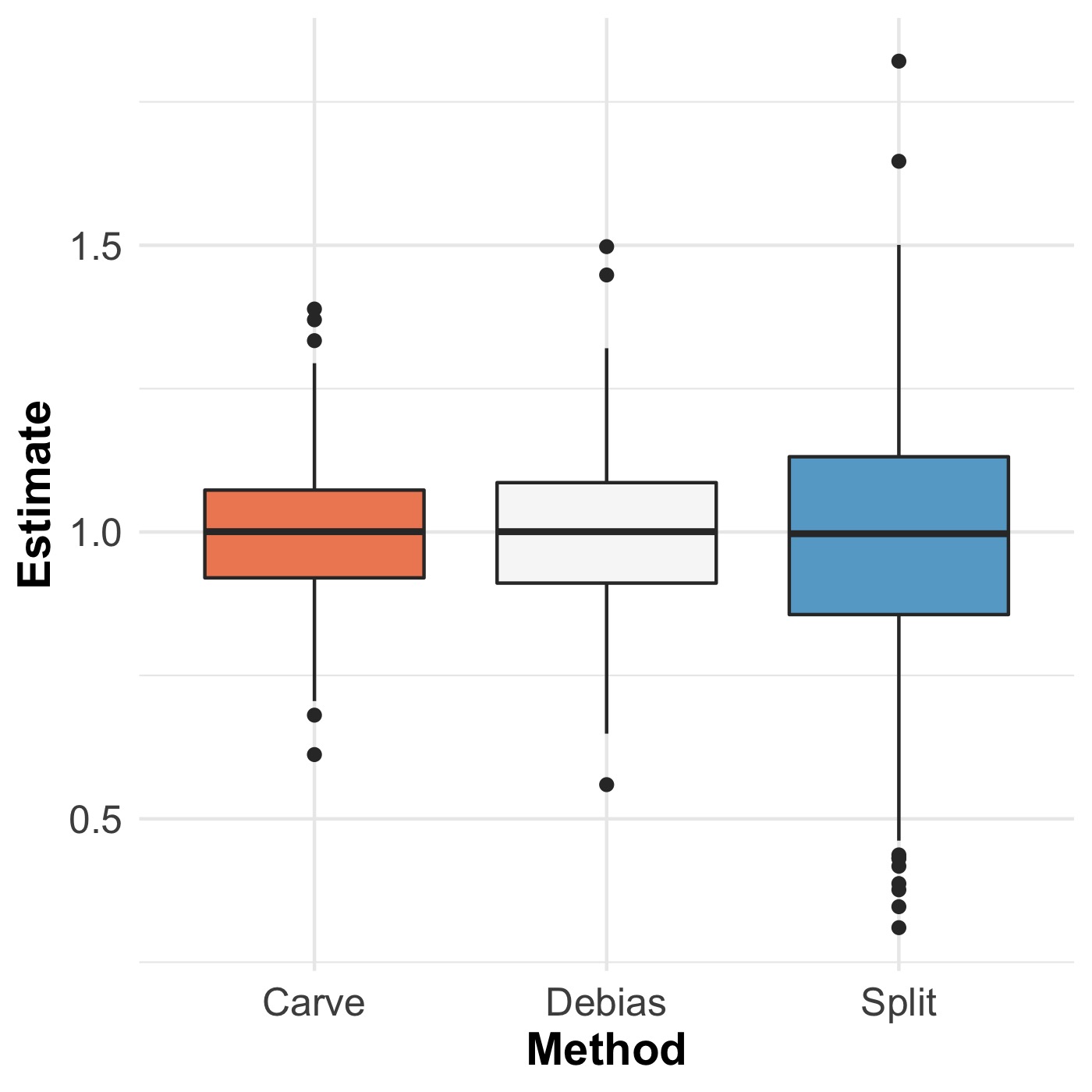
Next we extend our main ideas from this simple example to the more general setup. Before proceeding, we provide some numerical evidence for the effectiveness of our new estimator. We depict in Figure 2 the result of a simulation for $n=100$, $n_{1}=50$, and $1,000$ Monte Carlo samples. We compare our carved estimator against the two popular alternatives that were discussed earlier in the introduction, (1) the estimator based on data splitting, which simply uses the validation data $\mathcal{V}$ for estimation, and (2) the debiased LASSO estimator based on a one-step bias correction to the LASSO estimator. We elaborate on the generative scheme for the simulation as well as the implementation details for the other two alternatives in Section 4. Note that all the three estimators are centered around the true value $\alpha_{1}=1$. Especially, our new estimator removes the effect of selection bias, and has smallest variability among the three estimators.

We turn to our general setup, and outline our scheme to aggregate summary statistics from existing studies with data carving.

We begin by specifying the summary statistics involved in the construct of our estimator:

1. 1.

   Summary from model selection in existing studies: the support set of the LASSO estimator $E_{k}$, the penalty weights $\Lambda_{E_{k}}$, and the signs of the (nonzero) LASSO estimator for the selected covariates $s_{E_{k}}=\text{sign}(\widehat{\beta}_{k}^{\text{\;(L)}})$.

2. 2.

   Summary based on the first two moments from data in existing studies: the sample covariance matrices from the existing study $k$, based on the selected model $E_{k}$ and the observed sample of size $n_{k}$, which are equal to

   	$\displaystyle\widehat{\xi}_{k}=\left[\begin{array}[]{cc}\widehat{\xi}_{k,01}\\ \widehat{\xi}_{k,02}\end{array}\right]=$	$\displaystyle\frac{1}{n_{k}}\left[\begin{array}[]{c}D_{k}^{\prime}Y_{k}\\ X_{k,E_{k}}^{\prime}Y_{k}\end{array}\right],$
   	$\displaystyle\widehat{\Xi}_{k}=\ \left[\begin{array}[]{cc}\widehat{\Xi}_{k,11}&\widehat{\Xi}_{k,12}\\ \widehat{\Xi}_{k,21}&\widehat{\Xi}_{k,22}\end{array}\right]=$	$\displaystyle\frac{1}{n_{k}}\left[\begin{array}[]{cc}D_{k}^{\prime}D_{k}&D_{k}^{\prime}X_{k,E_{k}}\\ X_{k,E_{k}}^{\prime}D_{k}&X_{k,E_{k}}^{\prime}X_{k,E_{k}}\end{array}\right].$

   Note that $\widehat{\xi}_{k}$ has two blocks, one $s$-dimensional and the other $q_{k}$-dimensional. In a similar fashion, $\widehat{\Xi}_{k}$ is partitioned along the same dimensional structure.

First, we compute the least squares estimator

For a fixed vector $u\in\mathbb{R}^{k}$ and for $v\in\mathbb{R}^{k}$, let $\log(1+\frac{1}{uv})$ be a $\mathbb{R}^{k}$-valued vector whose $j$-th component equals

Denote by

the sample covariance matrix based on the selected covariates. We solve $\widehat{z}_{k}=\begin{pmatrix}\widehat{z}^{\prime}_{k,1}&\widehat{z}^{\prime}_{k,2}\end{pmatrix}^{\prime}$ from the following convex optimization problem:

where

Our carved estimator pools data from the existing study $k$ with the validation study, and is given by

Finally, we propose the aggregated estimator by taking a simple average of the $K$ carved estimators as

We conclude the section with some observations about our estimator.

In this section, we show how the debiasing approach in the first example can be generalized to our problem. In line with the first example, our carved estimator $\widehat{\alpha}_{k}^{\text{\; carve}}$ is obtained by conditioning on the selection event

which we observe after solving (2) on data $\mathcal{D}_{k}$. As before, we work with the selected model which assumes that data for the outcome variable are drawn as independent realizations from the conditional distribution

We proceed by fitting the selected model to $\mathcal{D}_{k}\cup\mathcal{V}$. Since we work under a fixed $\sigma^{2}$ setting, we will assume $\sigma^{2}=1$ for the sake of simplicity.

To develop the theory, we let

be our randomization variable, which is based on the LASSO solution $\widehat{\gamma}^{(L)}_{k}$. Let $E_{k}^{c}$ denote indices of covariates that are not selected by the LASSO in existing study $k$. In addition, we will also consider the statistic

Note, we need not observe the covariates that were not selected by the LASSO in the validation study. The statistics defined above only serve to provide a theoretical justification for our debiasing term. Proofs of our technical results are provided in Appendix A.

Lemma 3.4 notes that the variables $\widehat{\gamma}_{k}$, $\Gamma_{k}$ and $\omega_{k}$ admit an asymptotic linear representation in the selected model, if we ignored the impact of model selection and treated $E_{k}$ as a fixed set. Formally, this implies that these variables are distributed as Gaussian variables in the limit as the sample size $N_{k}\to\infty$.

Suppose that we condition this limiting Gaussian distribution on the selection event in (15). This gives us an asymptotic conditional distribution. Say that we denote this distribution by $\widetilde{L}_{N_{k}}$. Next, Proposition 3.5 derives a debiasing correction from this asymptotic conditional distribution as was done in the first example. Before stating this result, we let

denote the first moment of a Gaussian variable with mean $\alpha_{0}$ and covariance $\Sigma_{0}$ that is truncated to the region $\mathcal{H}_{0}$. Further, let $\Delta(\eta_{0})$ be the log-partition function for the related truncated Gaussian density at the natural parameter

Finally, for $\widehat{\Sigma}_{k}$ defined in (31), let $\Sigma_{k}=\mathbb{E}[\widehat{\Sigma}_{k}]$ be the population covariance.

The estimator in Theorem 3.5, however, does not admit direct computations due to lack of readily available expressions for the moments of a truncated Gaussian variable. To this end, we use the plug-in estimator $\widehat{\Sigma}_{k}$ and the inverse of $\widehat{\Sigma}_{k}$ for estimating $\Sigma_{k}$ and its inverse, respectively, and apply a Laplace-type approximation to facilitate a manageable calculation for this estimator. Deferring a rigorous justification of asymptotic unbiasedness to the next discussion, we complete the steps to numerically approximate our estimator through an easy-to-solve optimization. For

a Laplace approximation grants us the following

We replace the constrained optimization with the unconstrained version through a logarithmic barrier penalty to obtain

Applying the above approximation to our debiasing correction in Proposition 3.5 allows us to write

where $\widehat{z}_{k}$ is the solution in (12). This gives us the expression of our carved estimator in (13).

Our main result in the section, Theorem 3.10, establishes the asymptotic unbiasedness of our carved estimator.

Suppose that we have $N$ i.i.d. realizations of the response $\mathrm{y}\in\mathbb{R}$, the covariates for all existing studies $\mathrm{x}\in\mathbb{R}^{p_{1}+\cdots+p_{k}}$ and the treatment $\mathrm{d}\in\mathbb{R}^{s}$, such that $\mathrm{y}$ is drawn from the model in (1) with

Each of our existing studies, in particular, observes $N_{k}$ samples for the outcome and treatment along with a subset of covariates that are seen across all the studies. For the remaining section, we consider the following parameters

in our generation scheme, such that $\alpha_{0}$ and $\beta_{0,E_{0}}$ are constants and $a_{N}=o(\sqrt{N})$. We state the regularity and moment conditions on the data-generating mechanism below.

To start with, we impose asymptotic screening as a requirement on the model selection in the existing studies. This requirement is necessary to ensure that the bias from missing a true covariate is only negligible with growing sample size. The LASSO is an important example that satisfies the asymptotic screening requirement under conditions discussed at length by [15, 3]. Similar conditions are required by estimators which are aggregated over selected models, see for example the work by [22, 8].

The second condition below allows us to control the bias from the use of a Laplace-type approximation for our debiasing correction. The first part of the condition assumes the existence of an exponential moment in a neighborhood of zero. This is required to justify a Laplace-type approximation for probabilities involving the mean of $N$ i.i.d. variables, which in our case is $\bar{T}_{N_{k}}$ (as stated in Lemma 3.4) by setting $N=N_{k}$. The second part of the condition is required to extend this approximation to asymptotically linear variables with an added $o_{p}(1)$ error term, which we see in the left-hand side of the representation in Lemma 3.4.

The probability of selection can be written as the probability of a polyhedron:

where $A$ and $b$ are fixed matrices. The above characterization for the selection event has been proved in Proposition 4.2 of [20]. Our next condition allows us to replace the log-probability of selection with the log-probability of the polyhedron that is determined by matrices $A$ and $b$. In other words, this condition allows us to ignore the $o_{p}(1)$ remainder in the characterization for our selection event.

The final condition bounds the deviation of the sample estimate $\widehat{\Sigma}_{k}$ from the population parameter $\mathbb{E}[\widehat{\Sigma}_{k}]$.

For the remaining section, consider the parameters in (17) by fixing $N=N_{k}$.

The asymptotic variance of our estimator $\sqrt{N_{k}}\widehat{\alpha}_{k}^{\text{\; carve}}$, based on the observed Fisher information matrix, is

The expression for the estimated variance is detailed out in Proposition A.4, under Section A. Lemma 3.11 then quantifies the relative gain in variance of our estimator over splitting for each study $k$. Here, $\widehat{V}^{\;\text{split}}_{E_{k}}$ denotes the estimated variance of the least squares estimate when refitted on the validation data alone. Let $\widehat{V}_{j,E_{k}}^{\;\text{carve}}$ and $\widehat{V}^{\;\text{split}}_{j,E_{k}}$ be the $j$-th diagonal entry of the corresponding $s$-dimensional matrices, respectively.

Clearly, our carved estimator $\widehat{\alpha}_{k}^{\text{\; carve}}$ dominates the split estimators in variance. The variance of the averaged carved estimator, however, involves correlations between the refitted estimators from the selected models on any pair of existing studies in addition to the variances from each study. Heuristically, the correlation between a pair of split estimators, using the validation data alone, is expected to be larger than the carved counterpart. This is because the carved estimator also uses information from the independent samples in this pair of existing studies. Consider, for instance, the situation when each study reports the same model

Let the bound on the right-hand side of Lemma 3.11 be equal to $B_{k}$. Comparing the averaged carved estimator in (14) with the split estimator, the difference in the two variances is seen to be bounded below by

References

• [1] [author] Belloni, AlexandreA., Chernozhukov, VictorV. and Hansen, ChristianC. (2014). Inference on treatment effects after selection among high-dimensional controls. The Review of Economic Studies 81 608–650.
• [2] [author] Belloni, AlexandreA., Chernozhukov, VictorV. and Kato, KengoK. (2019). Valid post-selection inference in high-dimensional approximately sparse quantile regression models. Journal of the American Statistical Association 114 749–758.
• [3] [author] Bickel, Peter JP. J., Ritov, Ya’acovY. and Tsybakov, Alexandre BA. B. (2009). Simultaneous analysis of Lasso and Dantzig selector.
• [4] [author] Cai, TianxiT., Liu, MoleiM. and Xia, YinY. (2021). Individual data protected integrative regression analysis of high-dimensional heterogeneous data. Journal of the American Statistical Association just-accepted 1–34.
• [5] [author] Cattaneo, Matias DM. D., Jansson, MichaelM. and Newey, Whitney KW. K. (2018). Inference in linear regression models with many covariates and heteroscedasticity. Journal of the American Statistical Association 113 1350–1361.
• [6] [author] Chen, ShuxiaoS. and Bien, JacobJ. (2020). Valid inference corrected for outlier removal. Journal of Computational and Graphical Statistics 29 323–334.
• [7] Dwork, C., Feldman, V., Hardt, M., Pitassi, T., Reingold, O. and Roth, A. (2015). Generalization in Adaptive Data Analysis and Holdout Reuse. In Proceedings of the 28th International Conference on Neural Information Processing Systems - Volume 2. NIPS’15 2350–2358. MIT Press, Cambridge, MA, USA.
• [8] [author] Fei, ZheZ. and Li, YiY. (2021). Estimation and inference for high dimensional generalized linear models: A splitting and smoothing approach. The Journal of Machine Learning Research 22 2681–2712.
• [9] [author] Fithian, WilliamW., Sun, DennisD. and Taylor, JonathanJ. (2014). Optimal inference after model selection. arXiv preprint arXiv:1410.2597.
• [10] [author] Gao, Lucy LL. L., Bien, JacobJ. and Witten, DanielaD. (2020). Selective Inference for Hierarchical Clustering. arXiv preprint arXiv:2012.02936.
• [11] [author] Lee, Jason DJ. D., Liu, QiangQ., Sun, YuekaiY. and Taylor, Jonathan EJ. E. (2017). Communication-efficient sparse regression. The Journal of Machine Learning Research 18 115–144.
• [12] [author] Lee, Jason D.J. D., Sun, Dennis L.D. L., Sun, YuekaiY. and Taylor, Jonathan E.J. E. (2016). Exact post-selection inference with the lasso. The Annals of Statistics 44 907–927.
• [13] [author] Lin, Dan-YuD.-Y. and Zeng, DanielD. (2010). On the relative efficiency of using summary statistics versus individual-level data in meta-analysis. Biometrika 97 321–332.
• [14] [author] Maity, SubhaS., Sun, YuekaiY. and Banerjee, MoulinathM. (2019). Communication-efficient integrative regression in high-dimensions. arXiv preprint arXiv:1912.11928.
• [15] [author] Meinshausen, NicolaiN. and Bühlmann, PeterP. (2006). High-dimensional graphs and variable selection with the lasso.
• [16] [author] Panigrahi, SnigdhaS. (2019). Carving model-free inference. arXiv preprint arXiv:1811.03142.
• [17] [author] Panigrahi, SnigdhaS., MacDonald, Peter WP. W. and Kessler, DanielD. (2023). Approximate post-selective inference for regression with the group lasso. Journal of Machine Learning Research 24 1–49.
• [18] [author] Panigrahi, SnigdhaS. and Taylor, JonathanJ. (2018). Scalable methods for Bayesian selective inference. Electronic Journal of Statistics 12 2355–2400.
• [19] [author] Panigrahi, SnigdhaS. and Taylor, JonathanJ. (2022). Approximate selective inference via maximum likelihood. Journal of the American Statistical Association 1–11.
• [20] [author] Panigrahi, SnigdhaS., Taylor, JonathanJ. and Weinstein, AsafA. (2021). Integrative methods for post-selection inference under convex constraints. The Annals of Statistics 49 2803–2824.
• [21] [author] Park, Jay JHJ. J., Mogg, RobinR., Smith, Gerald EG. E., Nakimuli-Mpungu, EtheldredaE., Jehan, FyezahF., Rayner, Craig RC. R., Condo, JeanineJ., Decloedt, Eric HE. H., Nachega, Jean BJ. B., Reis, GilmarG. et al. (2021). How COVID-19 has fundamentally changed clinical research in global health. The Lancet Global Health 9 e711–e720.
• [22] [author] Schultheiss, ChristophC., Renaux, ClaudeC. and Bühlmann, PeterP. (2021). Multicarving for high-dimensional post-selection inference. Electronic Journal of Statistics 15 1695–1742.
• [23] [author] Stallard, NigelN. and Todd, SusanS. (2011). Seamless phase II/III designs. Statistical methods in medical research 20 623–634.
• [24] [author] Tang, LuL., Zhou, LingL. and Song, Peter X-KP. X.-K. (2020). Distributed simultaneous inference in generalized linear models via confidence distribution. Journal of Multivariate Analysis 176 104567.
• [25] [author] Tian, XiaoyingX. (2020). Prediction error after model search. The Annals of Statistics 48 763–784.
• [26] [author] Tian, XiaoyingX., Taylor, JonathanJ. et al. (2018). Selective inference with a randomized response. The Annals of Statistics 46 679–710.
• [27] [author] Tibshirani, RobertR. (1996). Regression shrinkage and selection via the lasso. Journal of the Royal Statistical Society. Series B (Methodological) 267–288.
• [28] [author] Wang, JingshenJ., He, XumingX. and Xu, GongjunG. (2020). Debiased Inference on Treatment Effect in a High-Dimensional Model. Journal of the American Statistical Association 115 442–454.
• [29] [author] Wolfson, MichaelM., Wallace, Susan ES. E., Masca, NicholasN., Rowe, GeoffG., Sheehan, Nuala AN. A., Ferretti, VincentV., LaFlamme, PhilippeP., Tobin, Martin DM. D., Macleod, JohnJ., Little, JulianJ. et al. (2010). DataSHIELD: resolving a conflict in contemporary bioscience—performing a pooled analysis of individual-level data without sharing the data. International journal of epidemiology 39 1372–1382.
A Proofs
A.1 Carved Estimator: first example
Suppose that ω1\omega_{1} and γ^1\widehat{\gamma}_{1} are Gaussian variables with the distribution stated in 1 and 2, i.e., the limiting distribution stated for these variables in 1 and 2 holds exactly. We note the following.
Proposition A.1.
Let α^1 carve\widehat{\alpha}_{1}^{\text{\;carve}} assume the value
α^1+{1ℝ+(sE1)⋅(1−ρ2)−1/2ρN1(Φ¯((λ−(1−ρ2)​N1​β^1)(1−ρ2)))−1ϕ((λ−(1−ρ2)​N1​β^1)(1−ρ2))\displaystyle\widehat{\alpha}_{1}+\Bigg\{1_{\mathbb{R}^{+}}(s_{E_{1}})\cdot(1-\rho^{2})^{-1/2}\dfrac{\rho}{\sqrt{N_{1}}}\left(\bar{\Phi}\left(\dfrac{(\lambda-(1-\rho^{2})\sqrt{N_{1}}\widehat{\beta}_{1})}{\sqrt{(1-\rho^{2})}}\right)\right)^{-1}{\phi\left(\dfrac{(\lambda-(1-\rho^{2})\sqrt{N_{1}}\widehat{\beta}_{1})}{\sqrt{(1-\rho^{2})}}\right)}
−1ℝ−(sE1)⋅(1−ρ2)−1/2ρN1(Φ((−λ−(1−ρ2)​N1​β^1)(1−ρ2)))−1ϕ((λ+(1−ρ2)​N1​β^1)(1−ρ2))}.\displaystyle-1_{\mathbb{R}^{-}}(s_{E_{1}})\cdot(1-\rho^{2})^{-1/2}\dfrac{\rho}{\sqrt{N_{1}}}\left(\Phi\left(\dfrac{(-\lambda-(1-\rho^{2})\sqrt{N_{1}}\widehat{\beta}_{1})}{\sqrt{(1-\rho^{2})}}\right)\right)^{-1}{\phi\left(\dfrac{(\lambda+(1-\rho^{2})\sqrt{N_{1}}\widehat{\beta}_{1})}{\sqrt{(1-\rho^{2})}}\right)}\Bigg\}.
Then, the following holds
𝔼⁡[α^1 carve]=α.\mathbb{E}\left[\widehat{\alpha}_{1}^{\text{\; carve}}\right]=\alpha.
Our proof proceeds in two steps.
Step 1: Fix
α^1 initial=α^1−(1−ρ2)−1​1N1⋅(ω1,1−ρ​ω1,2).\widehat{\alpha}_{1}^{\text{\;initial}}=\widehat{\alpha}_{1}-(1-\rho^{2})^{-1}\dfrac{1}{\sqrt{N_{1}}}\cdot(\omega_{1,1}-\rho\omega_{1,2}).
Note that
𝔼[α^1 initial|E^1=E1,sign(β^1(L))=sE1]=α.\mathbb{E}\left[\widehat{\alpha}_{1}^{\text{\; initial}}\;\Big\lvert\;\widehat{E}_{1}=E_{1},\;\text{sign}(\widehat{\beta}^{(L)}_{1})=s_{E_{1}}\right]=\alpha.
This observation follows by writing our conditioning event as
{E^1=E1,sign(β^1(L))=sE1}={sE1(ω1,2−ρω1,1)+sE1(1−ρ2)N1β^1−λ>0}.\left\{\widehat{E}_{1}=E_{1},\text{sign}(\widehat{\beta}^{(L)}_{1})=s_{E_{1}}\right\}=\left\{s_{E_{1}}(\omega_{1,2}-\rho\omega_{1,1})+s_{E_{1}}(1-\rho^{2})\sqrt{N_{1}}\widehat{\beta}_{1}-\lambda>0\right\}. (20)
Observe that the initial estimate is independent of
sE1​(ω1,2−ρ​ω1,1)+sE1​(1−ρ2)​N1​β^1−λ.s_{E_{1}}(\omega_{1,2}-\rho\omega_{1,1})+s_{E_{1}}(1-\rho^{2})\sqrt{N_{1}}\widehat{\beta}_{1}-\lambda.
Thus, we note that α^1 initial\widehat{\alpha}_{1}^{\text{\; initial}} is independent of our conditioning event, which gives us
𝔼[α^1initial|E^1=E1,sign(β^1(L))=sE1]=𝔼[α^1initial].\mathbb{E}\Big[\widehat{\alpha}_{1}^{\text{initial}}\ \Big\lvert\widehat{E}_{1}=E_{1},\text{sign}(\widehat{\beta}^{(L)}_{1})=s_{E_{1}}\Big]=\mathbb{E}\Big[\widehat{\alpha}_{1}^{\text{initial}}\Big].
Because
𝔼⁡[α^1initial]=α\mathbb{E}\Big[\widehat{\alpha}_{1}^{\text{initial}}\Big]=\alpha
for fixed set E1={1}E_{1}=\{1\}, we have an initial unbiased estimator.
Step 2: Conditioning further upon γ^1\widehat{\gamma}_{1} provides us the estimator
α^1 carve=𝔼[α^1−(1−ρ2)−11N1⋅(ω1,1−ρω1,2)|γ^1,sE1(ω1,2−ρω1,1)\displaystyle\widehat{\alpha}_{1}^{\text{\;carve}}=\mathbb{E}\Big[\widehat{\alpha}_{1}-(1-\rho^{2})^{-1}\dfrac{1}{\sqrt{N_{1}}}\cdot(\omega_{1,1}-\rho\omega_{1,2})\ \Big\lvert\widehat{\gamma}_{1},s_{E_{1}}(\omega_{1,2}-\rho\omega_{1,1})
+sE1(1−ρ2)N1β^1−λ>0]\displaystyle+s_{E_{1}}(1-\rho^{2})\sqrt{N_{1}}\widehat{\beta}_{1}-\lambda>0\Big]
=α^1−(1−ρ2)−11N1⋅𝔼[ω1,1−ρω1,2|γ^1,sE1(ω1,2−ρω1,1)\displaystyle=\widehat{\alpha}_{1}-(1-\rho^{2})^{-1}\dfrac{1}{\sqrt{N_{1}}}\cdot\mathbb{E}\Big[\omega_{1,1}-\rho\omega_{1,2}\ \lvert\ \widehat{\gamma}_{1},\;s_{E_{1}}(\omega_{1,2}-\rho\omega_{1,1})
+sE1(1−ρ2)N1β^1−λ>0],\displaystyle+s_{E_{1}}(1-\rho^{2})\sqrt{N_{1}}\widehat{\beta}_{1}-\lambda>0\Big],
an improvement over α^1 initial\widehat{\alpha}_{1}^{\text{\; initial}} through Rao-Blackwellization.
We compute the conditional expectation:
𝔼[ω1,1−ρω1,2|γ^1,sE1(ω1,2−ρω1,1)+sE1(1−ρ2)N1β^1−λ>0],\mathbb{E}\Big[\omega_{1,1}-\rho\omega_{1,2}\ \lvert\ \widehat{\gamma}_{1},\;s_{E_{1}}(\omega_{1,2}-\rho\omega_{1,1})+s_{E_{1}}(1-\rho^{2})\sqrt{N_{1}}\widehat{\beta}_{1}-\lambda>0\Big],
to obtain a final expression for our estimator. Note that we have, by construct,
𝔼[α^1 carve|E^1=E1,sign(β^1(L))=sE1]=α.\mathbb{E}\left[\widehat{\alpha}_{1}^{\text{\; carve}}\;\Big\lvert\;\widehat{E}_{1}=E_{1},\;\text{sign}(\widehat{\beta}^{(L)}_{1})=s_{E_{1}}\right]=\alpha.
Our claim in the Proposition now follows from the tower property of expectation. ∎
A.2 Carved Estimator: general problem
We give the proofs of the results in Section 3.
First, let
Σ^−k,k=1Nk​{XEkc′​(DXEk)+Xk,Ekc′​(DkXk,Ek)}\widehat{\Sigma}_{-k,k}=\frac{1}{N_{k}}\left\{X_{E_{k}^{c}}^{\prime}\begin{pmatrix}D&X_{E_{k}}\end{pmatrix}+X_{k,E_{k}^{c}}^{\prime}\begin{pmatrix}D_{k}&X_{k,E_{k}}\end{pmatrix}\right\}
and let Σ−k,k=𝔼⁡[Σ^−k,k]\Sigma_{-k,k}=\mathbb{E}[\widehat{\Sigma}_{-k,k}]. Also, let Σk=𝔼⁡[Σ^k]\Sigma_{k}=\mathbb{E}[\widehat{\Sigma}_{k}] where
Σ^k=1Nk​(nk​Ξ^k+(DXEk)′​(DXEk)).\widehat{\Sigma}_{k}=\frac{1}{N_{k}}\left(n_{k}\widehat{\Xi}_{k}+\begin{pmatrix}D&X_{E_{k}}\end{pmatrix}^{\prime}\begin{pmatrix}D&X_{E_{k}}\end{pmatrix}\right).
Then, define
T¯Nk\displaystyle\bar{T}_{N_{k}} =1Nk​(Σk−1​(DXEk)′​(y−D​α−XEk​βEk)(XEkc′−Σ−k,k​Σk−1​(DXEk)′)​(y−D​α−XEk​βEk)−(DX)′​(y−D​α−XEk​βEk))\displaystyle=\frac{1}{N_{k}}\begin{pmatrix}\Sigma^{-1}_{k}\begin{pmatrix}D&X_{E_{k}}\end{pmatrix}^{\prime}(y-D\alpha-X_{E_{k}}\beta_{E_{k}})\\ (X^{\prime}_{E_{k}^{c}}-\Sigma_{-k,k}\Sigma^{-1}_{k}\begin{pmatrix}D&X_{E_{k}}\end{pmatrix}^{\prime})(y-D\alpha-X_{E_{k}}\beta_{E_{k}})\\ -\begin{pmatrix}D&X\end{pmatrix}^{\prime}(y-D\alpha-X_{E_{k}}\beta_{E_{k}})\end{pmatrix}
+1Nk​(Σk−1​(DkXk,Ek)′​(yk−Dk​α−Xk,Ek​βEk)(Xk,Ekc′−Σ−k,k​Σk−1​(DkXk,Ek)′)​(yk−Dk​α−Xk,Ek​βEk)1rk​(DkXk)′​(yk−Dk​α−XEk​βEk)−(DkXk)′​(yk−Dk​α−Xk,Ek​βEk)).\displaystyle+\frac{1}{N_{k}}\begin{pmatrix}\Sigma^{-1}_{k}\begin{pmatrix}D_{k}&X_{k,E_{k}}\end{pmatrix}^{\prime}(y_{k}-D_{k}\alpha-X_{k,E_{k}}\beta_{E_{k}})\\ (X^{\prime}_{k,E_{k}^{c}}-\Sigma_{-k,k}\Sigma^{-1}_{k}\begin{pmatrix}D_{k}&X_{k,E_{k}}\end{pmatrix}^{\prime})(y_{k}-D_{k}\alpha-X_{k,E_{k}}\beta_{E_{k}})\\ \frac{1}{r_{k}}\begin{pmatrix}D_{k}&X_{k}\end{pmatrix}^{\prime}(y_{k}-D_{k}\alpha-X_{E_{k}}\beta_{E_{k}})-\begin{pmatrix}D_{k}&X_{k}\end{pmatrix}^{\prime}(y_{k}-D_{k}\alpha-X_{k,E_{k}}\beta_{E_{k}})\end{pmatrix}.
The proof of the Lemma closely follows Proposition 4.1 in [20], and hence we omit further details here. ∎
We state a useful Lemma before providing a proof for Proposition 3.5. Recall that
Σ^−k,k=1Nk​{XEkc′​(DXEk)+Xk,Ekc′​(DkXk,Ek)},\widehat{\Sigma}_{-k,k}=\frac{1}{N_{k}}\left\{X_{E_{k}^{c}}^{\prime}\begin{pmatrix}D&X_{E_{k}}\end{pmatrix}+X_{k,E_{k}^{c}}^{\prime}\begin{pmatrix}D_{k}&X_{k,E_{k}}\end{pmatrix}\right\},
and Σ−k,k=𝔼⁡[Σ^−k,k]\Sigma_{-k,k}=\mathbb{E}[\widehat{\Sigma}_{-k,k}]. Suppose that we rewrite (2) as
minimizeα,β​12​Nk​‖Y−D​α−X​β‖2+12​Nk​‖Yk−Dk​α−Xk​β‖2−ωk,1T​α−ωk,2T​β+‖Λ​β‖1\underset{\alpha,\beta}{\text{minimize}}\;\;\dfrac{1}{2\sqrt{N_{k}}}\|Y-D\alpha-X\beta\|^{2}+\dfrac{1}{2\sqrt{N_{k}}}\|Y_{k}-D_{k}\alpha-X_{k}\beta\|^{2}-\omega_{k,1}^{T}\alpha-\omega_{k,2}^{T}\beta+\|\Lambda\beta\|_{1} (21)
by using the randomization variable in (32). Fixing some more symbols, we let
ζk=(0s′(ΛEk​sEk)′)′,\zeta_{k}=\begin{pmatrix}0^{\prime}_{s}&(\Lambda_{E_{k}}s_{E_{k}})^{\prime}\end{pmatrix}^{\prime},
and denote by ZkZ_{k} the inactive components of subgradient variables from the ℓ1\ell_{1} penalty at the LASSO solution. Note that the K.K.T. mapping for (21) is equal to
ωk=[−Σ^k0−Σ^−k,k−I]​Nk​(γ^kΓ^k)+[Σ^k0Σ^−k,kΛEkc]​(Nk​γ^k(L)Zk)+(ζk0),\omega_{k}=\begin{bmatrix}-\widehat{\Sigma}_{k}&0\\ -\widehat{\Sigma}_{-k,k}&-I\end{bmatrix}\sqrt{N_{k}}\begin{pmatrix}\widehat{\gamma}_{k}\\ \widehat{\Gamma}_{k}\end{pmatrix}+\begin{bmatrix}\widehat{\Sigma}_{k}&0\\ \widehat{\Sigma}_{-k,k}&\Lambda_{E_{k}^{c}}\end{bmatrix}\begin{pmatrix}\sqrt{N_{k}}\widehat{\gamma}^{(L)}_{k}\\ Z_{k}\end{pmatrix}+\begin{pmatrix}\zeta_{k}\\ 0\end{pmatrix}, (22)
where the variables γ^k(L)\widehat{\gamma}^{(L)}_{k} and ZkZ_{k} satisfy
‖Zk‖≤1,sign​(β^k(L))=sEk.\|Z_{k}\|\leq 1,\ \text{sign}(\widehat{\beta}^{(L)}_{k})=s_{E_{k}}.
The next result derives an expression for the marginal asymptotic likelihood based on the limiting distribution of γ^k\widehat{\gamma}_{k} and γ^k(L)\widehat{\gamma}^{(L)}_{k}, before we condition on the event of selection.
Lemma A.2.
Marginally, the variables γ^k\widehat{\gamma}_{k}, γ^k(L)\widehat{\gamma}^{(L)}_{k} are asymptotically independent of Γ^k\widehat{\Gamma}_{k} and ZkZ_{k}. The marginal asymptotic likelihood, derived from the limiting distribution of γ^k\widehat{\gamma}_{k} and γ^k(L)\widehat{\gamma}^{(L)}_{k}, is proportional to
exp⁡(−Nk2​(γ^k−γk)′​Σk​(γ^k−γk))⋅exp⁡(−(1−rk)−1​rk​Nk2​(γ^k(L)−γ^k+1Nk​Σk−1​ζk)′CLOSE\displaystyle\exp\Bigg(-\frac{N_{k}}{2}(\widehat{\gamma}_{k}-\gamma_{k})^{\prime}\Sigma_{k}(\widehat{\gamma}_{k}-\gamma_{k})\Bigg)\cdot\exp\Bigg(-(1-r_{k})^{-1}r_{k}\frac{N_{k}}{2}\left(\widehat{\gamma}^{(L)}_{k}-\widehat{\gamma}_{k}+\frac{1}{\sqrt{N_{k}}}\Sigma^{-1}_{k}\zeta_{k}\right)^{\prime}
OPENΣk​(γ^k−γ^k+1Nk​Σk−1​ζk)).\displaystyle\Sigma_{k}\left(\widehat{\gamma}_{k}-\widehat{\gamma}_{k}+\frac{1}{\sqrt{N_{k}}}\Sigma^{-1}_{k}\zeta_{k}\right)\Bigg).
Using (22) together with the fact that Σ^k−Σk=op​(1)\widehat{\Sigma}_{k}-\Sigma_{k}=o_{p}(1), Σ^−k,k−Σ−k,k=op​(1)\widehat{\Sigma}_{-k,k}-\Sigma_{-k,k}=o_{p}(1) in our i.i.d. framework, we deduce that the variables γ^k(L)\widehat{\gamma}^{(L)}_{k} and ZkZ_{k} in this map admit the asymptotic representation:
Nk​γ^k(L)\displaystyle\sqrt{N}_{k}\widehat{\gamma}^{(L)}_{k} =Σk−1​ωk,E+Nk​γ^k−Σk−1​ζk+op​(1);\displaystyle=\Sigma^{-1}_{k}\omega_{k,E}+\sqrt{N_{k}}\widehat{\gamma}_{k}-\Sigma^{-1}_{k}\zeta_{k}+o_{p}(1); (23)
Zk\displaystyle Z_{k} =(ΛEkc)−1​(ωk,Ec−Σ−k,k​Σk−1​ωk,E+Σ−k,k​Σk−1​ζk+Nk​Γ^k)+op​(1).\displaystyle=(\Lambda_{E_{k}^{c}})^{-1}(\omega_{k,E^{c}}-\Sigma_{-k,k}\Sigma^{-1}_{k}\omega_{k,E}+\Sigma_{-k,k}\Sigma^{-1}_{k}\zeta_{k}+\sqrt{N}_{k}\widehat{\Gamma}_{k})+o_{p}(1).
We easily verify our claim by using the limiting marginal distribution of Nk​(γ^k−γk)\sqrt{N_{k}}(\widehat{\gamma}_{k}-\gamma_{k}), Nk​Γ^k\sqrt{N_{k}}\widehat{\Gamma}_{k}, and ωk\omega_{k}, that was derived in Lemma 3.4. ∎
We are ready to provide the proof of Proposition 3.5. The limiting distribution in Lemma 3.4 yields us an asymptotic debiasing term for the least squares estimator in the selected model after we condition on the selection event.
Proposition 3.5. We consider the following initial estimator
α^k initial=(1−rk)−1​α^k−(1−rk)−1​rk​e1′​(1Nk​Σk−1​ζk+γ^k(L)).\widehat{\alpha}_{k}^{\text{\; initial}}=(1-r_{k})^{-1}\widehat{\alpha}_{k}-(1-r_{k})^{-1}r_{k}e_{1}^{\prime}\left(\frac{1}{\sqrt{N_{k}}}\Sigma^{-1}_{k}\zeta_{k}+\widehat{\gamma}^{(L)}_{k}\right).
Observe, we have
𝔼[α^k initial|E^k=Ek,sign(β^k(L))=sEk]=α.\mathbb{E}\left[\widehat{\alpha}_{k}^{\text{\; initial}}\;\Big\lvert\;\widehat{E}_{k}=E_{k},\;\text{sign}(\widehat{\beta}^{(L)}_{k})=s_{E_{k}}\right]=\alpha.
This is because:
𝔼[α^k initial|E^k=Ek,sign(β^(L)k)=sEk]\displaystyle\mathbb{E}\left[\widehat{\alpha}_{k}^{\text{\; initial}}\;\Big\lvert\;\widehat{E}_{k}=E_{k},\;\text{sign}(\widehat{\beta}^{(L)}_{k})=s_{E_{k}}\right]
=𝔼⁡[(1−rk)−1​α^k−(1−rk)−1​rk​e1′​{1Nk​Σk−1​ζk+γ^k(L)}]\displaystyle=\mathbb{E}\left[(1-r_{k})^{-1}\widehat{\alpha}_{k}-(1-r_{k})^{-1}r_{k}e_{1}^{\prime}\left\{\frac{1}{\sqrt{N_{k}}}\Sigma^{-1}_{k}\zeta_{k}+\widehat{\gamma}^{(L)}_{k}\right\}\right]
=(1−rk)−1𝔼[α^k]−(1−rk)−1rke1′{1NkΣ−1kζk+𝔼[𝔼[γ^(L)k|γ^k]]}\displaystyle=(1-r_{k})^{-1}\mathbb{E}\left[\widehat{\alpha}_{k}\right]-(1-r_{k})^{-1}r_{k}e_{1}^{\prime}\left\{\frac{1}{\sqrt{N_{k}}}\Sigma^{-1}_{k}\zeta_{k}+\mathbb{E}\left[\mathbb{E}\left[\widehat{\gamma}^{(L)}_{k}\;\lvert\;\widehat{\gamma}_{k}\right]\right]\right\}
=(1−rk)−1​𝔼​[α^k]−(1−rk)−1​rk​e1′​{1Nk​Σk−1​ζk+𝔼⁡[γ^k−1Nk​Σk−1​ζk]}\displaystyle=(1-r_{k})^{-1}\mathbb{E}\left[\widehat{\alpha}_{k}\right]-(1-r_{k})^{-1}r_{k}e_{1}^{\prime}\left\{\frac{1}{\sqrt{N_{k}}}\Sigma^{-1}_{k}\zeta_{k}+\mathbb{E}\left[\widehat{\gamma}_{k}-\frac{1}{\sqrt{N_{k}}}\Sigma^{-1}_{k}\zeta_{k}\right]\right\}
=(1−rk)−1​𝔼​[α^k]−(1−rk)−1​rk​e1′​𝔼​[γ^k]=α.\displaystyle=(1-r_{k})^{-1}\mathbb{E}\left[\widehat{\alpha}_{k}\right]-(1-r_{k})^{-1}r_{k}e_{1}^{\prime}\mathbb{E}\left[\widehat{\gamma}_{k}\right]=\alpha.
Note, the first display uses the fact that our selection event can be rewritten as
{‖Zk‖∞≤1,sign​(β^k(L))=sEk}.\left\{\|Z_{k}\|_{\infty}\leq 1,\ \text{sign}(\widehat{\beta}^{(L)}_{k})=s_{E_{k}}\right\}.
That is, the conditional expectation of the initial estimator is equal to
𝔼[(1−rk)−1α^k−(1−rk)−1rke1′{1NkΣk−1ζk+γ^k(L)}|∥Zk∥∞≤1,sign(β^k(L))=sEk].\mathbb{E}\left[(1-r_{k})^{-1}\widehat{\alpha}_{k}-(1-r_{k})^{-1}r_{k}e_{1}^{\prime}\left\{\frac{1}{\sqrt{N_{k}}}\Sigma^{-1}_{k}\zeta_{k}+\widehat{\gamma}^{(L)}_{k}\right\}\;\Big\lvert\;\|Z_{k}\|_{\infty}\leq 1,\ \text{sign}(\widehat{\beta}^{(L)}_{k})=s_{E_{k}}\right].
The above expression is further equal to
𝔼⁡[(1−rk)−1​α^k−(1−rk)−1​rk​e1′​{1Nk​Σk−1​ζk+γ^k(L)}],\mathbb{E}\left[(1-r_{k})^{-1}\widehat{\alpha}_{k}-(1-r_{k})^{-1}r_{k}e_{1}^{\prime}\left\{\frac{1}{\sqrt{N_{k}}}\Sigma^{-1}_{k}\zeta_{k}+\widehat{\gamma}^{(L)}_{k}\right\}\right],
due to the independence between ZkZ_{k} and α^k initial\widehat{\alpha}_{k}^{\text{\; initial}} and between γ^k(L)\widehat{\gamma}^{(L)}_{k} and α^k initial\widehat{\alpha}_{k}^{\text{\; initial}} in the asymptotic limit, which follows directly from Lemma A.2. The second display uses the tower property of expectation. Using Lemma A.2 once again, we note that
𝔼[γ^k(L)|γ^k]=γ^k−1NkΣk−1ζk,\mathbb{E}\left[\widehat{\gamma}^{(L)}_{k}\;\Big\lvert\;\widehat{\gamma}_{k}\right]=\widehat{\gamma}_{k}-\frac{1}{\sqrt{N_{k}}}\Sigma^{-1}_{k}\zeta_{k},
in the penultimate display. Conditioning further upon γ^k\widehat{\gamma}_{k}, the complete sufficient statistic, our estimator in the claim is equal to
α^k carve=𝔼[α^k initial|γ^k,E^k=Ek,sign(β^k(L))=sEk].\widehat{\alpha}_{k}^{\text{\; carve}}=\mathbb{E}\left[\widehat{\alpha}_{k}^{\text{\; initial}}\;\Big\lvert\;\widehat{\gamma}_{k},\;\widehat{E}_{k}=E_{k},\;\text{sign}(\widehat{\beta}^{(L)}_{k})=s_{E_{k}}\right]. (24)
Obtaining an expression for the right-hand side estimate in (24), we have
𝔼[α^k initial|γ^k,E^k=Ek,sign(β^(L)k)=sEk]\displaystyle\mathbb{E}\left[\widehat{\alpha}_{k}^{\text{\; initial}}\;\Big\lvert\;\widehat{\gamma}_{k},\;\widehat{E}_{k}=E_{k},\;\text{sign}(\widehat{\beta}^{(L)}_{k})=s_{E_{k}}\right]
=(1−rk)−1⋅α^k−(1−rk)−1​rk​e1′​1Nk​Σk−1​ζk\displaystyle=(1-r_{k})^{-1}\cdot\widehat{\alpha}_{k}-(1-r_{k})^{-1}r_{k}e_{1}^{\prime}\frac{1}{\sqrt{N_{k}}}\Sigma^{-1}_{k}\zeta_{k}
−(1−rk)−1rk1Nk⋅e1′𝔼[Nkγ^(L)k|γ^k,sign(β^(L)k)=sEk].\displaystyle-(1-r_{k})^{-1}r_{k}\frac{1}{\sqrt{N_{k}}}\cdot e_{1}^{\prime}\mathbb{E}\left[\sqrt{N_{k}}\widehat{\gamma}^{(L)}_{k}\;\Big\lvert\;\widehat{\gamma}_{k},\;\text{sign}(\widehat{\beta}^{(L)}_{k})=s_{E_{k}}\right].
𝔼[Nkγ^k(L)|γ^k,sign(β^k(L))=sEk]=μℋ(Nkγ^k−Σk−1ζk,rk−1(1−rk)Σk−1),\mathbb{E}\left[\sqrt{N_{k}}\widehat{\gamma}^{(L)}_{k}\;\Big\lvert\;\widehat{\gamma}_{k},\;\text{sign}(\widehat{\beta}^{(L)}_{k})=s_{E_{k}}\right]=\mu_{\mathcal{H}}\left(\sqrt{N_{k}}\widehat{\gamma}_{k}-\Sigma^{-1}_{k}\zeta_{k},r_{k}^{-1}(1-r_{k})\Sigma^{-1}_{k}\right),
we obtain our estimator in the claim. ∎
A.3 Asymptotic properties of carved estimator
Before we provide a proof for the asymptotic unbiasedness of our estimator, we present a limiting value for the probability of selection. Fixing some notations, set γk=(α′βEk′)′\gamma_{k}=\begin{pmatrix}\alpha^{\prime}&\beta^{\prime}_{E_{k}}\end{pmatrix}^{\prime}. As per our parameterization in (17)
Nk​γk=aNk​γ0.\sqrt{N_{k}}\gamma_{k}=a_{N_{k}}\gamma_{0}.
Proposition A.3.
Suppose that the assumptions in Conditions 3.7 and 3.8 are met. Then, the probability of selection assumes the following limiting value:
limNk→∞1(aNk)2logℙ[E^k=Ek,sign(β^(L)k)=sEk]+infγ~,z~{12(γ~−γ0)′Σk(γ~−γ0)\displaystyle\lim_{N_{k}\to\infty}\frac{1}{(a_{N_{k}})^{2}}\log\mathbb{P}\left[\widehat{E}_{k}=E_{k},\;\text{sign}(\widehat{\beta}^{(L)}_{k})=s_{E_{k}}\right]+\displaystyle\inf_{\widetilde{\gamma},\widetilde{z}}\Big\{\dfrac{1}{2}(\widetilde{\gamma}-\gamma_{0})^{\prime}\Sigma_{k}(\widetilde{\gamma}-\gamma_{0})
+12(1−rk)−1rk(z~−γ~+1aNkΣk−1ζk)′Σk(z~−γ~+1aNkΣk−1ζk)+1(aNk)2BsEk(aNkz~)}−C0=0,\displaystyle+\dfrac{1}{2}(1-r_{k})^{-1}r_{k}(\widetilde{z}-\widetilde{\gamma}+\frac{1}{a_{N_{k}}}\Sigma_{k}^{-1}\zeta_{k})^{\prime}\Sigma_{k}(\widetilde{z}-\widetilde{\gamma}+\frac{1}{a_{N_{k}}}\Sigma_{k}^{-1}\zeta_{k})+\dfrac{1}{(a_{N_{k}})^{2}}B_{s_{E_{k}}}(a_{N_{k}}\widetilde{z})\Big\}-C_{0}=0,
where C0C_{0} is a constant free of γ0\gamma_{0}.
We have
limNk→∞1(aNk)2​{log⁡ℙ⁡[E^k=Ek,sign​(β^k(L))=sEk]−log⁡ℙ⁡[‖Zk‖∞≤1,sign​(β^k(L))=sEk]}=0,\lim_{N_{k}\to\infty}\frac{1}{(a_{N_{k}})^{2}}\left\{\log\mathbb{P}[\widehat{E}_{k}=E_{k},\;\text{sign}(\widehat{\beta}^{(L)}_{k})=s_{E_{k}}]-\log\mathbb{P}[\|Z_{k}\|_{\infty}\leq 1,\ \text{sign}(\widehat{\beta}^{(L)}_{k})=s_{E_{k}}]\right\}=0,
based on the K.K.T. conditions for the LASSO in (22). Using the asymptotic representation for the variables ZkZ_{k} and γ^k(L)\widehat{\gamma}^{(L)}_{k} in (23) and the condition in Condition 3.8, we note that
limNk→∞1(aNk)2​log⁡ℙ⁡[‖Zk‖∞≤1,sign​(β^k(L))=sEk]\lim_{N_{k}\to\infty}\frac{1}{(a_{N_{k}})^{2}}\log\mathbb{P}[\|Z_{k}\|_{\infty}\leq 1,\ \text{sign}(\widehat{\beta}^{(L)}_{k})=s_{E_{k}}]
is equal to
limNk→∞1(aNk)2{logℙ[sign(e2′(Σ−1kωk,E+Nkγ^k−Σ−1kζk))=sEk]\displaystyle\lim_{N_{k}\to\infty}\frac{1}{(a_{N_{k}})^{2}}\Big\{\log\mathbb{P}\left[\text{sign}(e_{2}^{\prime}(\Sigma^{-1}_{k}\omega_{k,E}+\sqrt{N_{k}}\widehat{\gamma}_{k}-\Sigma^{-1}_{k}\zeta_{k}))=s_{E_{k}}\right]
+logℙ[∥(ΛEkc)−1(ωk,Ec−Σ−k,kΣ−1kωk,E+Σ−k,kΣ−1kζk+NkΓ^k)∥∞≤1]}\displaystyle+\log\mathbb{P}\left[\|(\Lambda_{E_{k}^{c}})^{-1}(\omega_{k,E^{c}}-\Sigma_{-k,k}\Sigma^{-1}_{k}\omega_{k,E}+\Sigma_{-k,k}\Sigma^{-1}_{k}\zeta_{k}+\sqrt{N}_{k}\widehat{\Gamma}_{k})\|_{\infty}\leq 1\right]\Big\}
=limNk→∞T1,n+T2,n\displaystyle=\lim_{N_{k}\to\infty}T_{1,n}+T_{2,n}
where, for v1∈ℝsv_{1}\in\mathbb{R}^{s} and v2∈ℝqkv_{2}\in\mathbb{R}^{q_{k}}, e2′​(v1v2)=v2e_{2}^{\prime}\begin{pmatrix}v_{1}&v_{2}\end{pmatrix}=v_{2}. The assumption in Condition 3.7 allows to apply a large deviation limit for the two log-probabilities T1,nT_{1,n}, T2,nT_{2,n}. First, we note that
limNk→∞T1,n=limNk→∞1(aNk)2logℙ[sign(e2′(Σk−1ωk,E+Nkγ^k−Σk−1ζk))=sEk]\lim_{N_{k}\to\infty}T_{1,n}=\lim_{N_{k}\to\infty}\frac{1}{(a_{N_{k}})^{2}}\log\mathbb{P}\left[\text{sign}(e_{2}^{\prime}(\Sigma^{-1}_{k}\omega_{k,E}+\sqrt{N_{k}}\widehat{\gamma}_{k}-\Sigma^{-1}_{k}\zeta_{k}))=s_{E_{k}}\right]
agrees with
−infγ~,wE:sign​(e2′​(Σk−1​wE+γ~))=sEk{12(γ~−γ0)′Σk(γ~−γ0)+(1−rk)−1rk12wE′Σk−1wE}-\displaystyle\inf_{\widetilde{\gamma},w_{E}:\text{sign}(e_{2}^{\prime}(\Sigma^{-1}_{k}w_{E}+\widetilde{\gamma}))=s_{E_{k}}}\ \Big\{\dfrac{1}{2}(\widetilde{\gamma}-\gamma_{0})^{\prime}\Sigma_{k}(\widetilde{\gamma}-\gamma_{0})+(1-r_{k})^{-1}r_{k}\dfrac{1}{2}w_{E}^{\prime}\Sigma^{-1}_{k}w_{E}\Big\} (25)
up to an additive constant. Second, we note that the limiting distribution of the variables in T2,nT_{2,n} is free from γ0\gamma_{0}, and hereafter, let limNk→∞T2,n=C~\displaystyle\lim_{N_{k}\to\infty}T_{2,n}=\widetilde{C}.
At last, we apply a reparameterization to the optimizing variables wE→z~w_{E}\to\widetilde{z} such that z~=Σk−1​wE+γ~\widetilde{z}=\Sigma^{-1}_{k}w_{E}+\widetilde{\gamma} in (25). Thus, we note that the limiting value of the log-probability of selection is equal to
−infγ~,z~:sign​(z~2)=sEk{12(γ~−γ0)′Σk(γ~−γ0)+12(1−rk)−1rk(z~−γ~)′Σk(z~−γ~)}+C0,\displaystyle-\displaystyle\inf_{\widetilde{\gamma},\widetilde{z}:\text{sign}(\widetilde{z}_{2})=s_{E_{k}}}\ \Big\{\dfrac{1}{2}(\widetilde{\gamma}-\gamma_{0})^{\prime}\Sigma_{k}(\widetilde{\gamma}-\gamma_{0})+\dfrac{1}{2}(1-r_{k})^{-1}r_{k}(\widetilde{z}-\widetilde{\gamma})^{\prime}\Sigma_{k}(\widetilde{z}-\widetilde{\gamma})\Big\}+C_{0},
where C0C_{0} is a constant free of γ0\gamma_{0}. Because of convexity of the above optimization objective, we conclude that
limNk→∞{1(aNk)2logℙ[E^k=Ek,sign(β^(L)k)=sEk]+infγ~,z~{12(γ~−γ0)′Σk(γ~−γ0)\displaystyle\lim_{N_{k}\to\infty}\Big\{\frac{1}{(a_{N_{k}})^{2}}\log\mathbb{P}\left[\widehat{E}_{k}=E_{k},\;\text{sign}(\widehat{\beta}^{(L)}_{k})=s_{E_{k}}\right]+\displaystyle\inf_{\widetilde{\gamma},\widetilde{z}}\Big\{\dfrac{1}{2}(\widetilde{\gamma}-\gamma_{0})^{\prime}\Sigma_{k}(\widetilde{\gamma}-\gamma_{0})
+12(1−rk)−1rk(z~−γ~+1aNkΣk−1ζk)′Σk(z~−γ~+1aNkΣk−1ζk)+1(aNk)2BsEk(aNkz~)}−C0=0\displaystyle+\dfrac{1}{2}(1-r_{k})^{-1}r_{k}(\widetilde{z}-\widetilde{\gamma}+\frac{1}{a_{N_{k}}}\Sigma_{k}^{-1}\zeta_{k})^{\prime}\Sigma_{k}(\widetilde{z}-\widetilde{\gamma}+\frac{1}{a_{N_{k}}}\Sigma_{k}^{-1}\zeta_{k})+\dfrac{1}{(a_{N_{k}})^{2}}B_{s_{E_{k}}}(a_{N_{k}}\widetilde{z})\Big\}-C_{0}=0
to complete our proof. ∎
We introduce some important convex functions that we will need to prove Theorem 3.10. Let
DNk​(γ~)\displaystyle D_{N_{k}}(\widetilde{\gamma}) =12γ~′Σ^kγ~+infz~{12(1−rk)−1rk(z~−γ~+1aNkΣ^k−1ζk)′Σ^k(z~−γ~+1aNkΣ^k−1ζk)\displaystyle=\dfrac{1}{2}\widetilde{\gamma}^{\prime}\widehat{\Sigma}_{k}\widetilde{\gamma}+\displaystyle\inf_{\widetilde{z}}\Big\{\dfrac{1}{2}(1-r_{k})^{-1}r_{k}(\widetilde{z}-\widetilde{\gamma}+\frac{1}{a_{N_{k}}}\widehat{\Sigma}_{k}^{-1}\zeta_{k})^{\prime}\widehat{\Sigma}_{k}(\widetilde{z}-\widetilde{\gamma}+\frac{1}{a_{N_{k}}}\widehat{\Sigma}_{k}^{-1}\zeta_{k})
+1(aNk)2BsEk(aNkz~)},\displaystyle+\dfrac{1}{(a_{N_{k}})^{2}}B_{s_{E_{k}}}(a_{N_{k}}\widetilde{z})\Big\},
and let
𝒫~Nk​(η0)=supγ~γ~′​η0−DNk​(γ~),\widetilde{\mathcal{P}}_{N_{k}}(\eta_{0})=\displaystyle\sup_{\widetilde{\gamma}}\widetilde{\gamma}^{\prime}\eta_{0}-D_{N_{k}}(\widetilde{\gamma}), (26)
which is the convex conjugate for DNkD_{N_{k}}. Similarly, let
D˘Nk​(γ~)\displaystyle\breve{D}_{N_{k}}(\widetilde{\gamma}) =12γ~′Σkγ~+infz~{12(1−rk)−1rk(z~−γ~+1aNkΣk−1ζk)′Σk(z~−γ~+1aNkΣk−1ζk)\displaystyle=\dfrac{1}{2}\widetilde{\gamma}^{\prime}\Sigma_{k}\widetilde{\gamma}+\displaystyle\inf_{\widetilde{z}}\Big\{\dfrac{1}{2}(1-r_{k})^{-1}r_{k}(\widetilde{z}-\widetilde{\gamma}+\frac{1}{a_{N_{k}}}\Sigma_{k}^{-1}\zeta_{k})^{\prime}\Sigma_{k}(\widetilde{z}-\widetilde{\gamma}+\frac{1}{a_{N_{k}}}\Sigma_{k}^{-1}\zeta_{k})
and let 𝒫˘Nk\breve{\mathcal{P}}_{N_{k}} be the corresponding convex conjugate.
Theorem 3.10. First, we note that our carved estimator is equal to
1aNkNkα^k carve=e1′Σ^k−1∇DNk(1aNkNkγ^k),\frac{1}{a_{N_{k}}}\sqrt{N_{k}}\widehat{\alpha}_{k}^{\text{\; carve}}=e_{1}^{\prime}\widehat{\Sigma}^{-1}_{k}\nabla D_{N_{k}}\left(\frac{1}{a_{N_{k}}}\sqrt{N_{k}}\widehat{\gamma}_{k}\right), (27)
where ∇DNk\nabla D_{N_{k}} is the gradient of DNkD_{N_{k}}. This is because
∇DNk​(γ~)=Σ^k​γ~−(1−rk)−1​rk​Σ^k​(z∗​(γ~)−γ~+1aNk​Σ^k−1​ζk),\displaystyle\nabla D_{N_{k}}(\widetilde{\gamma})=\widehat{\Sigma}_{k}\widetilde{\gamma}-(1-r_{k})^{-1}r_{k}\widehat{\Sigma}_{k}\left(z^{*}(\widetilde{\gamma})-\widetilde{\gamma}+\frac{1}{a_{N_{k}}}\widehat{\Sigma}_{k}^{-1}\zeta_{k}\right),
where
z∗​(γ~)\displaystyle z^{*}(\widetilde{\gamma}) =arginfz{12(1−rk)−1rk(z~−γ~+1aNkΣ^k−1ζk)′Σ^k(z~−γ~+1aNkΣ^k−1ζk)\displaystyle=\text{arginf}_{z}\;\Big\{\dfrac{1}{2}(1-r_{k})^{-1}r_{k}\left(\widetilde{z}-\widetilde{\gamma}+\frac{1}{a_{N_{k}}}\widehat{\Sigma}_{k}^{-1}\zeta_{k}\right)^{\prime}\widehat{\Sigma}_{k}\left(\widetilde{z}-\widetilde{\gamma}+\frac{1}{a_{N_{k}}}\widehat{\Sigma}_{k}^{-1}\zeta_{k}\right)
and z∗​(1aNk​Nk​γ^k)=1aNk​Nk​z^kz^{*}\left(\frac{1}{a_{N_{k}}}\sqrt{N_{k}}\widehat{\gamma}_{k}\right)=\frac{1}{a_{N_{k}}}\sqrt{N_{k}}\widehat{z}_{k}, where z^k\widehat{z}_{k} is defined in (12).
Also, define
𝒫~0,Nk​(η0)=1(aNk)2​log⁡ℙ⁡[E^k=Ek,sign​(β^k(L))=sEk]+12​η0′​Σk−1​η0,\widetilde{\mathcal{P}}_{0,N_{k}}(\eta_{0})=\frac{1}{(a_{N_{k}})^{2}}\log\mathbb{P}\left[\widehat{E}_{k}=E_{k},\;\text{sign}(\widehat{\beta}^{(L)}_{k})=s_{E_{k}}\right]+\frac{1}{2}\eta^{\prime}_{0}\Sigma^{-1}_{k}\eta_{0},
where η0=Σk​γ0\eta_{0}=\Sigma_{k}\gamma_{0}. Let λmax\lambda_{\text{max}} and λmin\lambda_{\text{min}} be the largest and smallest eigen-value of Σ^k\widehat{\Sigma}_{k}. Now, we have
𝔼[∥1aNkNk(α^k carve−α)∥2|E^k=Ek,sign(β^(L)k)=sEk]\displaystyle\mathbb{E}\left[\Big\|\frac{1}{a_{N_{k}}}\sqrt{N_{k}}(\widehat{\alpha}_{k}^{\text{\; carve}}-\alpha)\Big\|^{2}\Big\lvert\widehat{E}_{k}=E_{k},\text{sign}(\widehat{\beta}^{(L)}_{k})=s_{E_{k}}\right]
≤1λmin2​(Σ^k)𝔼[∥∇𝒫~Nk−1(1aNkNkγ^k)−Σ^kγ0∥2|E^k=Ek,sign(β^(L)k)=sEk]\displaystyle\leq\dfrac{1}{\lambda^{2}_{\text{min}}(\widehat{\Sigma}_{k})}\mathbb{E}\left[\Big\|\nabla\widetilde{\mathcal{P}}_{N_{k}}^{-1}\left(\frac{1}{a_{N_{k}}}\sqrt{N_{k}}\widehat{\gamma}_{k}\right)-\widehat{\Sigma}_{k}\gamma_{0}\Big\|^{2}\Big\lvert\widehat{E}_{k}=E_{k},\text{sign}(\widehat{\beta}^{(L)}_{k})=s_{E_{k}}\right]
≤C2λmin2​(Σ^k)𝔼[∥1aNkNkγ^k−∇𝒫~Nk(Σ^kγ0)∥2|E^k=Ek,sign(β^(L)k)=sEk]\displaystyle\leq\dfrac{C^{2}}{\lambda^{2}_{\text{min}}(\widehat{\Sigma}_{k})}\mathbb{E}\left[\Big\|\frac{1}{a_{N_{k}}}\sqrt{N_{k}}\widehat{\gamma}_{k}-\nabla\widetilde{\mathcal{P}}_{N_{k}}(\widehat{\Sigma}_{k}\gamma_{0})\Big\|^{2}\Big\lvert\widehat{E}_{k}=E_{k},\text{sign}(\widehat{\beta}^{(L)}_{k})=s_{E_{k}}\right]
≤C2λmin2​(Σ^k){𝔼[∥1aNkNkγ^k−∇𝒫~0,Nk(Σkγ0)∥2|E^k=Ek,sign(β^(L)k)=sEk]\displaystyle\leq\dfrac{C^{2}}{\lambda^{2}_{\text{min}}(\widehat{\Sigma}_{k})}\Bigg\{\mathbb{E}\left[\Big\|\frac{1}{a_{N_{k}}}\sqrt{N_{k}}\widehat{\gamma}_{k}-\nabla\widetilde{\mathcal{P}}_{0,N_{k}}(\Sigma_{k}\gamma_{0})\Big\|^{2}\Big\lvert\widehat{E}_{k}=E_{k},\text{sign}(\widehat{\beta}^{(L)}_{k})=s_{E_{k}}\right]
+𝔼[∥∇𝒫˘Nk(Σkγ0)−∇𝒫~Nk(Σ^kγ0)∥2|E^k=Ek,sign(β^(L)k)=sEk]\displaystyle+\mathbb{E}\left[\Big\|\nabla\breve{\mathcal{P}}_{N_{k}}(\Sigma_{k}\gamma_{0})-\nabla\widetilde{\mathcal{P}}_{N_{k}}(\widehat{\Sigma}_{k}\gamma_{0})\Big\|^{2}\Big\lvert\widehat{E}_{k}=E_{k},\text{sign}(\widehat{\beta}^{(L)}_{k})=s_{E_{k}}\right]
+∥∇𝒫˘Nk(Σkγ0)−∇𝒫~0,Nk(Σkγ0)∥2}.\displaystyle+\Big\|\nabla\breve{\mathcal{P}}_{N_{k}}(\Sigma_{k}\gamma_{0})-\nabla\widetilde{\mathcal{P}}_{0,N_{k}}(\Sigma_{k}\gamma_{0})\Big\|^{2}\Bigg\}.
The second display uses (26) and (27) to deduce:
e1′Σ^−1k∇𝒫~Nk−1(1aNkNkγ^k)\displaystyle e_{1}^{\prime}\widehat{\Sigma}^{-1}_{k}\nabla\widetilde{\mathcal{P}}_{N_{k}}^{-1}\left(\frac{1}{a_{N_{k}}}\sqrt{N_{k}}\widehat{\gamma}_{k}\right) =e1′Σ^−1k∇DNk(1aNkNkγ^k)=1aNkNkα^k carve.\displaystyle=e_{1}^{\prime}\widehat{\Sigma}^{-1}_{k}\nabla D_{N_{k}}\left(\frac{1}{a_{N_{k}}}\sqrt{N_{k}}\widehat{\gamma}_{k}\right)=\frac{1}{a_{N_{k}}}\sqrt{N_{k}}\widehat{\alpha}_{k}^{\text{\; carve}}.
The third display uses the fact that ∇𝒫~Nk−1\nabla\widetilde{\mathcal{P}}_{N_{k}}^{-1} is Lipschitz with constant CC where C=(1−rk)−1​λmax​(Σ^k)C=(1-r_{k})^{-1}\lambda_{\text{max}}(\widehat{\Sigma}_{k}). The last display follows after using the standard triangle inequality for decomposing the preceding expectation. For the decomposition shown in the last display, it is easy note that the expectation in the first term is O⁡(1)O(1). Observe that ∇𝒫~Nk​(⋅)\nabla\widetilde{\mathcal{P}}_{N_{k}}(\cdot), in the second display, is Lipschitz, because it is the gradient of the conjugate of a strongly convex function. Using the fact that Σ^k−Σk=op​(1)\widehat{\Sigma}_{k}-\Sigma_{k}=o_{p}(1) in our i.i.d. framework, jointly with the condition in Assumption 3.9, we deduce that the expected value of the second term is O⁡(1)O(1). The third term converges to 00 by using the convexity of 𝒫~0,Nk\widetilde{\mathcal{P}}_{0,N_{k}} together with the pointwise convergence shown by Proposition A.3. This completes our proof. ∎
We turn to deriving a feasible value for the observed Fisher information matrix in order to estimate the variance of the carved estimator. To this end, the limiting value for the probability of selection in Proposition A.3 gives rise to an approximate log-partition function in terms of η0=Σk​γ0\eta_{0}=\Sigma_{k}\gamma_{0}, the natural parameters in the asymptotic distribution of the refitted least squares estimation after conditioning on the selection event.
Letting
Nk​η=aNk​η0,\sqrt{N}_{k}\eta=a_{N_{k}}\eta_{0},
observe that the approximate log-partition function based on Proposition A.3 is given by:
aNk22η0′Σ−1kη0−aNk2⋅infγ~,z~{12(γ~−Σ−1kη0)′Σk(γ~−Σ−1kη0)\displaystyle\frac{a^{2}_{N_{k}}}{2}\eta_{0}^{\prime}\Sigma^{-1}_{k}\eta_{0}-a_{N_{k}}^{2}\cdot\displaystyle\inf_{\widetilde{\gamma},\widetilde{z}}\Big\{\dfrac{1}{2}(\widetilde{\gamma}-\Sigma^{-1}_{k}\eta_{0})^{\prime}\Sigma_{k}(\widetilde{\gamma}-\Sigma^{-1}_{k}\eta_{0}) (28)
+12(1−rk)−1rk(z~−γ~+1aNkΣk−1ζk)′Σk(z~−γ~+1aNkΣk−1ζk)+1(aNk)2BsEk(aNkz)}\displaystyle+\dfrac{1}{2}(1-r_{k})^{-1}r_{k}(\widetilde{z}-\widetilde{\gamma}+\frac{1}{a_{N_{k}}}\Sigma_{k}^{-1}\zeta_{k})^{\prime}\Sigma_{k}(\widetilde{z}-\widetilde{\gamma}+\frac{1}{a_{N_{k}}}\Sigma_{k}^{-1}\zeta_{k})+\dfrac{1}{(a_{N_{k}})^{2}}B_{s_{E_{k}}}(a_{N_{k}}z)\Big\}
=Nk2η′Σ−1kη−infγ,z{12(Nkγ−NkΣ−1kη)′Σk(Nkγ−NkΣ−1kη)\displaystyle=\frac{N_{k}}{2}\eta^{\prime}\Sigma^{-1}_{k}\eta-\displaystyle\inf_{\gamma,z}\Big\{\dfrac{1}{2}(\sqrt{N_{k}}\gamma-\sqrt{N_{k}}\Sigma^{-1}_{k}\eta)^{\prime}\Sigma_{k}(\sqrt{N_{k}}\gamma-\sqrt{N_{k}}\Sigma^{-1}_{k}\eta)
+12​(1−rk)−1​rk​(Nk​z−Nk​γ+Σk−1​ζk)′​Σk​(Nk​z−Nk​γ+Σk−1​ζk)\displaystyle+\dfrac{1}{2}(1-r_{k})^{-1}r_{k}(\sqrt{N_{k}}z-\sqrt{N_{k}}\gamma+\Sigma_{k}^{-1}\zeta_{k})^{\prime}\Sigma_{k}(\sqrt{N_{k}}z-\sqrt{N_{k}}\gamma+\Sigma_{k}^{-1}\zeta_{k})
+BsEk(Nkz)}.\displaystyle+B_{s_{E_{k}}}(\sqrt{N_{k}}z)\Big\}.
The last display is derived by reparameterizing aNk​γ~=Nk​γa_{N_{k}}\widetilde{\gamma}=\sqrt{N_{k}}\gamma, aNk​z~=Nk​za_{N_{k}}\widetilde{z}=\sqrt{N_{k}}z. Denote by 𝒫Nk​(η)\mathcal{P}_{N_{k}}(\eta) the approximate log-partition function in the last display, which we use to obtain an operational expression for the observed Fisher information matrix next. We plug in the sample estimate for the unknown covariance Σk\Sigma_{k} to estimate the value of the observed Fisher information matrix. Proposition A.4 outlines the derivation of this estimator. The symbol e1e_{1} in the claim denotes a qk+sq_{k}+s dimensional block diagonal matrix, where the first ss-dimensional matrix along the diagonal is the identity matrix with ss columns and the second qkq_{k}-dimensional matrix is a matrix of all zeros.
Proposition A.4.
Based on the approximate value for the log-partition function in (28), the inverse of the observed Fisher information matrix assumes the following expression:
e1′​((1−rk)−1​Σ^k−1−(1−rk)−2​rk2​((1−rk)−1​rk​Σ^k+∇2BsEk​(Nk​z^k))−1)​e1.\displaystyle e_{1}^{\prime}\left((1-r_{k})^{-1}\widehat{\Sigma}^{-1}_{k}-(1-r_{k})^{-2}r^{2}_{k}\left((1-r_{k})^{-1}r_{k}\widehat{\Sigma}_{k}+\nabla^{2}B_{s_{E_{k}}}(\sqrt{N_{k}}\widehat{z}_{k})\right)^{-1}\right)e_{1}.
Using the approximate expression for the log-partition function in (28), the observed Fisher information submatrix is equal to
e1′Σ^k∇2𝒫Nk(Σ^kγ^k carve)Σ^ke1=e1′Σ^k∇γ∗Σ^ke1e_{1}^{\prime}\widehat{\Sigma}_{k}\nabla^{2}\mathcal{P}_{N_{k}}(\widehat{\Sigma}_{k}\widehat{\gamma}_{k}^{\text{\; carve}})\widehat{\Sigma}_{k}e_{1}=e_{1}^{\prime}\widehat{\Sigma}_{k}\nabla\gamma^{*}\widehat{\Sigma}_{k}e_{1}
where γ∗\gamma^{*} equals
argsupγNkγ′Σ^kNkγ^k carve−12Nkγ′Σ^kNkγ\displaystyle\displaystyle\arg\sup_{\gamma}\sqrt{N_{k}}\gamma^{\prime}\widehat{\Sigma}_{k}\sqrt{N_{k}}\widehat{\gamma}_{k}^{\text{\; carve}}-\dfrac{1}{2}\sqrt{N_{k}}\gamma^{\prime}\widehat{\Sigma}_{k}\sqrt{N_{k}}\gamma (29)
−infz{12(1−rk)−1rk(Nkz−Nkγ+Σ^k−1ζk)′Σ^k(Nkz−Nkγ+Σ^k−1ζk)\displaystyle-\displaystyle\inf_{z}\Big\{\dfrac{1}{2}(1-r_{k})^{-1}r_{k}(\sqrt{N_{k}}z-\sqrt{N_{k}}\gamma+\widehat{\Sigma}_{k}^{-1}\zeta_{k})^{\prime}\widehat{\Sigma}_{k}(\sqrt{N_{k}}z-\sqrt{N_{k}}\gamma+\widehat{\Sigma}_{k}^{-1}\zeta_{k})
Solving (29) gives us
Σ^k​Nk​γ^k carve=Σ^k​Nk​γ∗+(1−rk)−1​rk​Σ^k​(Nk​γ∗−Σ^k−1​ζk−Nk​z^k),\widehat{\Sigma}_{k}\sqrt{N_{k}}\widehat{\gamma}_{k}^{\text{\; carve}}=\widehat{\Sigma}_{k}\sqrt{N_{k}}\gamma^{*}+(1-r_{k})^{-1}r_{k}\widehat{\Sigma}_{k}\left(\sqrt{N_{k}}\gamma^{*}-\widehat{\Sigma}_{k}^{-1}\zeta_{k}-\sqrt{N_{k}}\widehat{z}_{k}\right),
(1−rk)−1​rk​Σ^k​(Nk​z^k−Nk​γ∗+Σ^k−1​ζk)+∇BsEk​(Nk​z^k)=0.(1-r_{k})^{-1}r_{k}\widehat{\Sigma}_{k}\left(\sqrt{N_{k}}\widehat{z}_{k}-\sqrt{N_{k}}\gamma^{*}+\widehat{\Sigma}_{k}^{-1}\zeta_{k}\right)+\nabla B_{s_{E_{k}}}(\sqrt{N_{k}}\widehat{z}_{k})=0.
The former equations yields us γ∗=γ^k\gamma^{*}=\widehat{\gamma}_{k}, using the expression for our carved estimator. Taking further derivatives, we obtain
∇γ∗z^k=((1−rk)−1​rk​Σ^k+∇2BsEk​(Nk​z^k))−1​(1−rk)−1​rk​Σ^k,\nabla_{\gamma^{*}}\widehat{z}_{k}=\left((1-r_{k})^{-1}r_{k}\widehat{\Sigma}_{k}+\nabla^{2}B_{s_{E_{k}}}(\sqrt{N_{k}}\widehat{z}_{k})\right)^{-1}(1-r_{k})^{-1}r_{k}\widehat{\Sigma}_{k},
∇γ∗=((1−rk)−1​Σ^k−(1−rk)−1​rk​Σ^k​∇γ∗z^k)−1\displaystyle\nabla\gamma^{*}=\left((1-r_{k})^{-1}\widehat{\Sigma}_{k}-(1-r_{k})^{-1}r_{k}\widehat{\Sigma}_{k}\nabla_{\gamma^{*}}\widehat{z}_{k}\right)^{-1}
=((1−rk)−1​Σ^k−(1−rk)−1​rk​Σ^k​((1−rk)−1​rk​Σ^k+∇2BsEk​(Nk​z^k))−1​(1−rk)−1​rk​Σ^k)−1.\displaystyle=\Big((1-r_{k})^{-1}\widehat{\Sigma}_{k}-(1-r_{k})^{-1}r_{k}\widehat{\Sigma}_{k}\left((1-r_{k})^{-1}r_{k}\widehat{\Sigma}_{k}+\nabla^{2}B_{s_{E_{k}}}(\sqrt{N_{k}}\widehat{z}_{k})\right)^{-1}(1-r_{k})^{-1}r_{k}\widehat{\Sigma}_{k}\Big)^{-1}.
Then, the inverse for the Fisher information matrix is given by:
(1−rk)−1​Σ^k−1−(1−rk)−2​rk2​((1−rk)−1​rk​Σ^k+∇2BsEk​(Nk​z^k))−1,\displaystyle(1-r_{k})^{-1}\widehat{\Sigma}^{-1}_{k}-(1-r_{k})^{-2}r^{2}_{k}\left((1-r_{k})^{-1}r_{k}\widehat{\Sigma}_{k}+\nabla^{2}B_{s_{E_{k}}}(\sqrt{N_{k}}\widehat{z}_{k})\right)^{-1},
which directly leads to our claim in the Proposition. ∎
B Carved Estimator for Logistic Regression
Fixing some notations, let
p⁡(x)=exp⁡(x)1+exp⁡(x)p(x)=\dfrac{\exp(x)}{1+\exp(x)}
for x∈ℝx\in\mathbb{R}.
Suppose that we observe a binary response variable which assumes values in {0,1}\{0,1\}. Introducing some notations, we let
for x∈ℝx\in\mathbb{R}. Let π⁡(Dk​α+Xk​β)∈ℝnk\pi(D_{k}\alpha+X_{k}\beta)\in\mathbb{R}^{n_{k}} be the vector with
p⁡((Dk(i))′​α+(Xk(i))′​β)p\left((D_{k}^{(i)})^{\prime}\alpha+(X_{k}^{(i)})^{\prime}\beta\right)
as its ithi^{\text{th}} component. We let
ℓ⁡(Yk,π⁡(Dk​α+Xk​β))\displaystyle\ell(Y_{k},\pi(D_{k}\alpha+X_{k}\beta)) =−∑i=1nk{Yk(i)logp((Dk(i))′α+(Xk(i))′β)\displaystyle=-\sum_{i=1}^{n_{k}}\Big\{Y_{k}^{(i)}\log p\left((D_{k}^{(i)})^{\prime}\alpha+(X_{k}^{(i)})^{\prime}\beta\right)
+(1−Yk(i))log(1−p((Dk(i))′α+(Xk(i))′β))}\displaystyle+(1-Y_{k}^{(i)})\log\left(1-p\left((D_{k}^{(i)})^{\prime}\alpha+(X_{k}^{(i)})^{\prime}\beta\right)\right)\Big\}
denote the logistic loss based on nkn_{k} samples of the kthk^{\text{th}} existing study.
In each existing study, we apply the logistic regression with an added LASSO penalty to estimate
γ^k (L)=(α^k (L)β^k (L))=arg⁡minα∈ℝs,β∈ℝpk​{1rk​Nk​ℓ​(Yk,π⁡(Dk​α+Xk​β))+||Λk​β||1},\widehat{\gamma}^{\text{\;(L)}}_{k}=\begin{pmatrix}\widehat{\alpha}^{\text{\;(L)}}_{k}\\ \widehat{\beta}^{\text{\;(L)}}_{k}\end{pmatrix}=\underset{\alpha\in\mathbb{R}^{s},\beta\in\mathbb{R}^{p_{k}}}{\arg\min}\left\{\frac{1}{r_{k}\sqrt{N_{k}}}\ell(Y_{k},\pi(D_{k}\alpha+X_{k}\beta))+||\Lambda_{k}\beta||_{1}\right\}, (30)
where α^k (L)∈ℝs\widehat{\alpha}^{\text{\;(L)}}_{k}\in\mathbb{R}^{s}, β^k (L)∈ℝqk\widehat{\beta}^{\text{\;(L)}}_{k}\in\mathbb{R}^{q_{k}} for k=1,2,…,Kk=1,2,\ldots,K. Denote by EkE_{k} the support set of β^k (L)\widehat{\beta}_{k}^{\text{\;(L)}}.
Next, we identify the summary statistics that we require from each existing study, and give the form of our estimator. Consider the following summary information from existing study kk.
1. 1.
Summary from model selection: the support set of the LASSO estimator EkE_{k}, the penalty weights ΛEk\Lambda_{E_{k}}, and the signs of the (nonzero) LASSO estimator for the selected covariates sEk=sign​(β^k (L))s_{E_{k}}=\text{sign}(\widehat{\beta}_{k}^{\text{\;(L)}}).
2. 2.
Summary from the first two moments in the selected model: the MLE in the selected model EkE_{k}
ξ^k:=[ξ^k,01ξ^k,02]\widehat{\xi}_{k}:=\left[\begin{array}[]{cc}\widehat{\xi}_{k,01}\\ \widehat{\xi}_{k,02}\end{array}\right]
and the estimated information matrix in the same model
Ξ^k:=[Ξ^k,11Ξ^k,12Ξ^k,21Ξ^k,22]=\displaystyle\widehat{\Xi}_{k}:=\ \left[\begin{array}[]{cc}\widehat{\Xi}_{k,11}&\widehat{\Xi}_{k,12}\\ \widehat{\Xi}_{k,21}&\widehat{\Xi}_{k,22}\end{array}\right]= 1nk​[Dk′​Wk​(ξ^k)​DkDk′​Wk​(ξ^k)​Xk,EkXk,Ek′​Wk​(ξ^k)​DkXk,Ek′​Wk​(ξ^k)​Xk,Ek],\displaystyle\frac{1}{n_{k}}\left[\begin{array}[]{cc}D_{k}^{\prime}W_{k}(\widehat{\xi}_{k})D_{k}&D_{k}^{\prime}W_{k}(\widehat{\xi}_{k})X_{k,E_{k}}\\ X_{k,E_{k}}^{\prime}W_{k}(\widehat{\xi}_{k})D_{k}&X_{k,E_{k}}^{\prime}W_{k}(\widehat{\xi}_{k})X_{k,E_{k}}\end{array}\right],
where Wk​(ξ^k)∈ℝnk×nkW_{k}(\widehat{\xi}_{k})\in\mathbb{R}^{n_{k}\times n_{k}} denotes a diagonal matrix with
πi​([DkXk,Ek]​ξ^k)​(1−πi​([DkXk,Ek]​ξ^k))\pi_{i}\left(\begin{bmatrix}D_{k}&X_{k,E_{k}}\end{bmatrix}\widehat{\xi}_{k}\right)\left(1-\pi_{i}\left(\begin{bmatrix}D_{k}&X_{k,E_{k}}\end{bmatrix}\widehat{\xi}_{k}\right)\right)
in its ithi^{\text{th}} diagonal entry. Note that ξ^k\widehat{\xi}_{k} and Ξ^k\widehat{\Xi}_{k} are partitioned along the same dimensional structure as before.
Let ξ^\widehat{\xi} be the MLE in the selected model, using observations in the validation study, and let Σ^=D′​W​(ξ^)​D\widehat{\Sigma}=D^{\prime}W(\widehat{\xi})D be the (corresponding) estimated information matrix in the same model. Denote by W⁡(ξ^)∈ℝn×nW(\widehat{\xi})\in\mathbb{R}^{n\times n} a diagonal matrix with
πi​([DXEk]​ξ^)​(1−πi​([DXEk]​ξ^))\pi_{i}\left(\begin{bmatrix}D&X_{E_{k}}\end{bmatrix}\widehat{\xi}\right)\left(1-\pi_{i}\left(\begin{bmatrix}D&X_{E_{k}}\end{bmatrix}\widehat{\xi}\right)\right)
in its ithi^{\text{th}} diagonal entry. First, we aggregate the estimated information matrix as
Σ^k=nk​Ξ^k+(DXEk)′​W​(ξ^)​(DXEk),\widehat{\Sigma}_{k}=n_{k}\widehat{\Xi}_{k}+\begin{pmatrix}D&X_{E_{k}}\end{pmatrix}^{\prime}W(\widehat{\xi})\begin{pmatrix}D&X_{E_{k}}\end{pmatrix}, (31)
and then we compute the aggregated MLE as
γ^k=((α^k)′(β^k)′)′=Σ^k−1​(nk​Ξ^k​ξ^k+Σ^​ξ^).\widehat{\gamma}_{k}=\begin{pmatrix}(\widehat{\alpha}_{k})^{\prime}&(\widehat{\beta}_{k})^{\prime}\end{pmatrix}^{\prime}=\widehat{\Sigma}_{k}^{-1}\left(n_{k}\widehat{\Xi}_{k}\widehat{\xi}_{k}+\widehat{\Sigma}\widehat{\xi}\right).
Hereon, our carved estimator takes the exact same form as (13). That is, we solve the optimization in (12) by using the aggregated MLE γ^k\widehat{\gamma}_{k}, and information matrix Σ^k\widehat{\Sigma}_{k}.
Our theory follows the exact steps as before once we define our randomization variable as
ωk\displaystyle\omega_{k} =((ωk,1)′(ωk,2)′)′;ωk,1∈ℝs,ωk,2∈ℝpk\displaystyle=\begin{pmatrix}(\omega_{k,1})^{\prime}&(\omega_{k,2})^{\prime}\end{pmatrix}^{\prime};\;\omega_{k,1}\in\mathbb{R}^{s},\omega_{k,2}\in\mathbb{R}^{p_{k}} (32)
=∂∂γ​(1Nk​ℓ​(Yk,π⁡(Dk​α+Xk​β))+1Nk​ℓ​(Y,π⁡(D​α+X​β))CLOSE\displaystyle=\dfrac{\partial}{\partial\gamma}\Bigg(\frac{1}{\sqrt{N_{k}}}\ell(Y_{k},\pi(D_{k}\alpha+X_{k}\beta))+\frac{1}{\sqrt{N_{k}}}\ell(Y,\pi(D\alpha+X\beta))
−1rk​Nkℓ(Yk,π(Dkα+Xkβ)))|γ^k(L),\displaystyle-\frac{1}{r_{k}\sqrt{N_{k}}}\ell(Y_{k},\pi(D_{k}\alpha+X_{k}\beta))\Bigg)\Bigg\lvert_{\widehat{\gamma}^{(L)}_{k}},
and set
Γ^k=1Nk​{Xk,Ekc′​(Yk−π⁡(Dk​α^k+Xk​β^k))+XEkc′​(Y−π⁡(D​α^k+X​β^k))}.\widehat{\Gamma}_{k}=\dfrac{1}{N_{k}}\left\{X^{\prime}_{k,E_{k}^{c}}(Y_{k}-\pi(D_{k}\widehat{\alpha}_{k}+X_{k}\widehat{\beta}_{k}))+X^{\prime}_{E_{k}^{c}}(Y-\pi(D\widehat{\alpha}_{k}+X\widehat{\beta}_{k}))\right\}.
Then, we have the asymptotic linear representation as stated in Lemma 3.4, and the rest of the theory proceeds as before.