CPHT-RR001.012022
Random Field Model and Parisi-Sourlas Supersymmetry
Apratim Kaviraja,b,c, Emilio Trevisanib,d
aInstitut de Physique Théorique Philippe Meyer,
b
Laboratoire de Physique de l’Ecole normale supérieure, ENS,
Université PSL, CNRS, Sorbonne Université, Université de Paris, F-75005 Paris, France
c DESY Hamburg, Theory Group, Notkestraße 85, D-22607 Hamburg, Germany
d CPHT, CNRS, Ecole Polytechnique, IP Paris, F-91128 Palaiseau, France
March 2022
Abstract
We use the RG framework set up in [1] to explore the theory with a random field interaction. According to the Parisi-Sourlas conjecture this theory admits a fixed point with emergent supersymmetry which is related to the pure Lee-Yang CFT in two less dimensions. We study the model using replica trick and Cardy variables in where the RG flow is perturbative. Allowed perturbations are singlets under the symmetry that permutes the replicas. These are decomposed into operators with different scaling dimensions: the lowest dimensional part, ‘leader’, controls the RG flow in the IR; the other operators, ‘followers’, can be neglected. The leaders are classified into: susy-writable, susy-null and non-susy-writable according to their mixing properties. We construct low lying leaders and compute the anomalous dimensions of a number of them. We argue that there is no operator that can destabilize the SUSY RG flow in . This agrees with the well known numerical result for critical exponents of Branched Polymers (which are in the same universality class as the random field model) that match the ones of the pure Lee-Yang fixed point according to dimensional reduction in all . Hence this is a second strong check of the RG framework that was previously shown to correctly predict loss of dimensional reduction in random field Ising model.
1 Introduction
Physical systems with randomly distributed impurities can be modelled through disordered quantum field theories. Random Field (RF) models constitute a class of such theories where a disorder field is coupled to a local order parameter. We are interested in the simplest RF models described by the following continuous action
| (1.1) |
where the disorder field is coupled to a single scalar field for a given potential . This continuous description conveniently captures the physics of the theory near the phase transition, where the microscopic details of the model are inconsequential. Typically the disorder field is chosen to be Gaussian, with a zero mean. Physical observables are obtained by taking correlation functions for a given configuration of and then computing their average over the disorder. The disordered coupling is relevant if . This is called Harris criterion. Since (with ) close to the usual upper critical dimension, the disorder is strongly relevant and changes the universality class of the critical system.
A notable example of RF theories is the Random Field Ising Model (RFIM), which can be defined on the lattice by adding to the usual Ising model a term which couples the disorder field to a local Ising spin. This corresponds to in the action above. In this paper we focus on another important example: Random Field model (denoted RF model), where we set . We discuss it in a moment. The analysis for both and potentials appeared in a shorter paper [2].
In [3] it was first suggested that RF theories of the type (1.1) have a phase transition with an interesting feature: its critical point is related to that of the same system without disorder in dimension. This was explained by a conjecture due to Parisi and Sourlas in 1979 [4], in the context of RFIM. The conjecture has two essential parts:
- 1.
Emergence of supersymmetry: The IR fixed point of the RF theory is equivalent to the fixed point of a nonunitary supersymmetric theory (with supercharges that do not transform in a spinor representation). This is the Parisi-Sourlas CFT.
- 2.
Dimensional reduction: The correlation functions of the SUSY CFT restricted to a hyperplane are equal to those of a dimensional CFT with the same action as the disordered model but without the disorder.
The above implies that critical exponents of a RF model should be the same as those of a CFTd-2. However this is not always true as found in the RFIM case from a number of numerical studies. Indeed the model shows dimensional reduction from [5, 6] but not for [7] or .11 1 The case cannot work as there is no phase transition for Ising model in 1d. This means that one of the two parts of Parisi-Sourlas mechanism should stop working for RFIM at some intermediate dimension. In [8] part 2 of the conjecture was explored in the framework of axiomatic CFTs. It was shown that there was no issue with dimensional reduction in the Parisi-Sourlas SUSY CFT.
Part 1 of the conjecture was explored in [1]. A perturbative RG framework was set up to study the model. It was shown that the emergent SUSY fixed point ot the RFIM is in fact unstable below a critical dimension. The key points of the analysis were the following:
- •
One represents the RF model by using a replica Lagrangian. In this formulation, the disorder field is integrated out and one is left with a pure quantum field theory of coupled fields in the limit .
- •
The fields do not have a well defined scaling even in the Gaussian theory (for ). This is problematic for RG purposes. It is thus convenient to perform a linear map in field space [9], dubbed Cardy transform, which gives rise to a set of fields with well defined scaling dimensions.
- •
Near the upper critical dimension the model is described by a Gaussian action perturbed by a weakly relevant interaction. This gives rise to an IR fixed point equivalent to the Parisi-Sourlas SUSY CFT.
- •
There is an infinite number of other perturbations, that are irrelevant close to . The fixed point would become unstable if any of these perturbations becomes marginal at .
- •
The perturbations are all -singlets i.e. invariant under the symmetry that permutes the replicas. These singlets (like the fields themselves) do not have well defined scaling dimensions. Indeed, after Cardy transform, they can be written as a sum of operators of different dimensions. The lowest dimensional part of the singlet is called “leader operator”, the other parts are named “followers”.
- •
The leader operators fully control the behaviour of the -singlet perturbations in the IR. It is therefore enough to study the anomalous dimensions of leaders (in a theory —dubbed — where all followers are set to zero) to know if the -singlet perturbations are relevant or irrelevant.
- •
The leader operators are further classified into 3 categories: susy-writable, susy-null and non-susy-writable.
- •
The anomalous dimensions of a number of low dimension leader operators in each category were computed in [1]. This showed that a few -singlet perturbations do become marginal at some critical dimensions estimated as thus rendering the fixed point unstable at .
We review the framework in detail in section 2. The result of the above RG framework nicely explains when and why dimensional reduction works for the RFIM. If the framework is correct it should also be applicable to other known cases giving results consistent with the numerical predictions. In this paper we test the above framework on the RF model.
Let us briefly review some features of this model. First let us consider the pure version of the RF theory. This is described by the scalar theory which has upper critical dimension . This theory has a microscopical description realized by considering the Ising model in an imaginary magnetic field. The critical properties of the model are captured by the well-known Lee-Yang universality class [10, 11, 12, 13].
Once we add the disorder, by the Harris criterion, the fixed point must be in a different universality class. Interestingly the universality class of the RF fixed point describes the critical properties of branched polymers in a solution. Branched polymers are defined as polymers —long chains of single units called monomers— which branch into other polymers. Depending on the interactions between the parts of the chain they can appear in extended or collapsed configurations. One can study the properties of the polymers near the transition between these two phases. It is also possible to define the branched polymers on the lattice as connected clusters of sites called ‘Lattice Animals’. The number of their possible configurations and their average size, scale with some critical exponents that are known from Monte-Carlo for all dimensions [14, 15]. Lubensky and Isaacson [16] proposed that branched polymers can also be described in field theory with the limit of a Replica Lagrangian with cubic interaction that allows perturbative computations in (see appendix A for a review). Parisi and Sourlas [17] showed that this Lagrangian also describes the RF model. Through the Parisi-Sourlas conjecture this is related to Lee-Yang fixed point without disorder in dimensions. Critical exponents in the lower dimensional theory are known from both perturbative computations (in dimensions) and Monte-Carlo. They agree with the branched polymer critical exponents, showing that both parts of Parisi-Sourlas conjecture indeed work for this model.
The fact that Parisi-Sourlas conjecture works in this model is supported by the result of Brydges and Imbrie [18] who found a manifestly supersymmetric model of Branched polymers, where the dimensional reduction can be rigorously shown (see [19] for a review). However that analysis does not explain why a generic non-supersymmetric model should also have a SUSY fixed point, namely why SUSY breaking perturbations are irrelevant (see App. A.4 of [1] for more details on this point). Therefore one important goal of this paper is to explain using the RG analysis of [1] how RF fixed point flows to a stable SUSY fixed point that admits dimensional reduction in all allowed dimensions .
The rest of the paper is organized as follows: In section 2 we review the RG framwork of [1] focusing on the RF theory. We introduce ‘leader’ and ‘follower’ operators and show how the SUSY fixed point arises. In section 3 we classify all the leader operators into three categories. In each category we compute the anomalous dimensions of the ones that have low classical dimensions and break SUSY. In section 4 we use the results to argue that the SUSY fixed point is stable. We conclude in section 5. There are four appendices that show various technical details and computations.
2 The RG flow of random field models
In this section we investigate how SUSY emerges in the RG flow of a RF model. In order to study this question we follow the logic of [1], summarized in Fig.1. We start the next subsection by reviewing how to compute quenched disorder correlation functions through the method of replicas [20]. We then define a transformation in field space (first introduced by Cardy [9]) which makes the scaling properties of the UV Gaussian fixed point more transparent. In section 2.2 we explain how to do RG in these new variables and we show that the IR properties of the model are captured by the “leader theory”, which is specified by a simpler Lagrangian .
Thanks to this formulation we can easily classify the spectrum of the theory and see which perturbations are relevant and whether they give rise to a SUSY IR fixed point or not. In subsection 2.3 we will focus on the case in which is small and we will easily show that can be mapped to a SUSY model with Parisi-Sourlas supersymmetry. Finally in subsection 2.4 we explain that the resulting SUSY model can be dimensionally reduced to a non-SUSY theory in dimensions. In principle, when is of order one, new relevant SUSY breaking operators could destabilize the SUSY fixed point, as it happens for the RFIM. This scenario for RF will be considered and ruled out in sections 3 and 4.
2.1 Method of replicas and Cardy transform
Quenched averaged correlators are defined by first averaging over the field and in the end over the random magnetic field
| (2.1) |
where overbar denotes the disorder average with distribution , is the random field action introduced in (1.1) and is a function of the field , e.g. . In this paper we will focus on a gaussian disorder distribution . Because of the presence of the denominator , equation (2.1) is notoriously complicated to compute. The method of replicas is a prescription to compute these correlation functions by eliminating the factor .
The idea is to multiply and divide the integrand of (2.1) by . The resulting equation is independent of , thus we can take the limit , where the denominator . The in the numerator is instead considered as a product of partition functions for fields which combine with the original functional integral where is renamed . The net result is that we get rid of the denominator at the price of having replica fields . The advantage of this trick is that the average over is now just a Gaussian integral which can be performed giving
| (2.2) |
| (2.3) |
We can also generalize this construction to compute the disorder-average of a product of several correlators as follows
| (2.4) |
where the result is independent of the choice of indices as long as they are all different. While the definition (2.1) eludes the standard QFT framework because of the average over disorder, the reformulation in (2.2-2.4) is conveniently written in terms a QFT of coupled fields (the only subtlety being the limit ). This formulation is thus well suited to study the RG of the theory.
From the quadratic part of we obtain the propagator
| (2.5) |
where is an matrix whose all elements are equal to one. We see that, in the limit , the two terms in the r.h.s. of (2.5) have different scalings in . This in turns implies that the fields at the UV fixed point do not possess a definite scaling dimension. The idea of Cardy [9] is to disentangle the two scaling behaviors through a linear transformation in field space. The Cardy transform is defined as follows
| (2.6) |
with . By construction, the variables are not independent and satisfy the constraint . The quadratic Lagrangian in limit thus becomes
| (2.7) |
where from now on we leave implicit the sum over , where runs from to . We borrowed the notation from [1] and the superscript ‘free’ denotes the case.
The transformed fields , , have now well-defined scaling dimensions:
| (2.8) |
Notice that the dimension of is one unit below the unitarity bound, signaling that the resulting theory is actually non unitary. By inverting the kinetic term we then obtain the free propagators, which are now scale-covariant
| (2.9) |
Here is an matrix whose components are all equal to one. In this new basis the powers and of (2.5) appear separated. Notice that to get such a neat separation we had to work at . Let us show that indeed order terms are not important to study the RG of the random field model.
To model this problem we consider a Lagrangian independent of perturbed by a relevant operator with dimension , which is multiplied by a coupling of order (which we think as a small parameter),
| (2.10) |
with the UV cutoff energy scale and . For our problem is a Lagrangian obtained by setting (e.g. the Gaussian Lagrangian , where we are also allowed to turn on any number of perturbations discussed in the next sections) while is any relevant operator that enters at order (there are many of such operators e.g. ). We want to see what happens to the RG of when is small and understand how we are supposed to think of a line of theories parametrized by which are smoothly connected to the theory (indeed this is what we are supposed to have when when we use the method of replica). This is non trivial since there are two conflicting effects: on one hand looks unimportant because is small in the UV, on the other hand is a relevant coupling, thus it should grow and become important in the IR. Let us explain how we should understand these fighting effects. The coupling —which in the UV was order-— grows along the RG and becomes order-1 at a scale
| (2.11) |
At scales the flow is no longer perturbative and we have no means to predict the fate of the theory (which may flow to a gapped phase or to new fixed point). Formula (2.11) thus tells us that any fix point of the RG is ultimately unstable with respect to order perturbations. So in practice no matter how small is, the coupling will eventually become large and destabilize the RG. One could then think that it is not possible to find a smooth interpolation between the theories with and the one. On the contrary, in the following we explain how this can be done.
Indeed, as approaches zero, the scale (2.11) (at which ) becomes smaller and smaller. In practice the instabilities are only triggered at parametrically large distances. This indicates that we should only focus on the regime . Because of the IR cutoff at these scales we can only reach approximate scale invariance. However by lowering we are able to make the approximate scale invariant region larger and larger, finally reaching a true fixed point at (which is the one of theory).
Very importantly in the regime all (2.10) contributions are perturbative. They appear as a Taylor series in which can be dropped when taking the limit . It is thus possible to drop them from the start. In summary from now on we are allowed to consider the theory at strictly and drop all perturbations that which are proportional to . This is going to be assumed in the rest of the paper.
2.2 RG in Cardy variables
In the previous section we showed how the gaussian Lagrangian at takes a nice form in Cardy variables. The next step is to consider the RG of the theory.
Independently of the form of the potential, the replica action (2.2) is symmetric. In order to study the RG of (2.2) we should consider all possible perturbations compatible with , and possible extra symmetries if they are not broken by the form of the potential. E.g. in [1] a quartic potential was considered, which allowed for an extra symmetry. In this work we will consider a cubic potential in (2.2), thus the symmetry will not be present.
symmetric preturbations are easily written in terms of the replica fields, e.g.
| (2.12) |
and so on. On the other hand in order to use the results of the previous section, we need to rewrite the -singlet operators in Cardy variables. To do so we simply use (2.6) and we set . The lowest dimensional singlets in Cardy basis are the following quadratic operators22 2 In principle one can also consider the perturbation . This however does not play any role, since it can be reabsorbed in the Gaussian Lagrangian (2.7) by a shift of fields, . Indeed, as we will explain in App. B, this perturbation is equivalent to the perturbation in theory, which is also discarded because it can be reabsorbed by a shift of .
| (2.13) |
We see that and generate the Gaussian Lagrangian of (2.7).33 3 It is important to see that the two terms belong to different -singlets, so the relative coefficient is allowed to change along an -preserving RG flow. This is not a problem since the IR fixed point is independent of such relative rescaling, as it is explained in section 3 of [1]. Since they generate the kinetic terms, they are by definition always marginal. The perturbation instead has scaling dimensions , thus it is always strongly relevant. It takes the role of a mass term, which we need to tune to zero in order to reach an IR fixed point. The next perturbation is which appears due to the potential of the perturbed UV action (2.3). In Cardy variables it takes the form
| (2.14) |
Here the subscript of the square brackets indicate the bare dimensions of the composite operators computed by summing the dimensions of the fields in (2.8). We thus conclude that the singlet can be written as a sum of operators of different dimensions, which is actually a recurrent feature of the model. While looking very exotic, this feature should be expected. Indeed, as we stressed in the previous section, the fields which are used to define the singlets do not have a well-defined scaling dimension. Thus we do not expect to find that combinations of give operators with definite dimensions. The quadratic operators in (2.13) should be considered as exceptions to this rule. In general a given singlet perturbation is written in Cardy basis as a sum of operators of different dimensions
| (2.15) |
where we distinguish its lowest dimensional piece which we call leader from all the higher dimensional terms which we dub followers, where the follower has dimension -units bigger than . As it should be clear from what follows, this difference in dimension does not renormalize, so the difference between the dimensions of a leader and its followers is the same in the UV and in the IR.
It is easy to see that leaders play a much more important role than followers to characterize the IR properties of the RG. This can be shown in two steps. First, due to symmetry, the form of the multiplet must be preserved when integrating out degrees of freedom. E.g. if we introduce a momentum cutoff and we integrate out the momentum shell , where , the form of is not allowed to change, meaning that the relative coefficients between and the remain fixed and only the overall coupling is allowed to change,
| (2.16) |
Here is the coupling associated to at a scale , while is new coupling after integrating out the momentum shell from . Second, when we rescale back to initial form of the action we see that the relative coefficients get rescaled differently and follower operators are more and more suppressed as we go to the IR,
| (2.17) |
In particular in the deep IR, and all follower operators are set to zero with respect to the leader. We can define an RG equation for the perturbation as the variation of in the RG scale . Close to the fixed point this can be linearized as follows,
| (2.18) |
From this construction it should be clear that the eigenvalue can be computed in a very simple way: it is obtained as where is the the scaling dimension of the leader operator computed in a simpler theory —which we call — defined by dropping all follower operators. This is a remarkable conclusion. It gives us a very simple algorithm to check if an perturbation is relevant or not. The strategy is to construct the perturbations, map them in Cardy variables and drop all the follower contributions. By studying the anomalous dimensions of the leader operators in the theory we are then able to see if and thus the perturbation falls off in the IR, or if and the perturbation grows. E.g. to study the IR effect of the perturbation , we should only consider its leader piece , which has bare dimension and thus gives rise to a weakly relevant perturbation in dimensions. In the next section we will detail what happens to the IR fixed point of this RG flow. Before ending this section we shall make a final remark about the theory.
Of course, as it is written, equation (2.18) works when there are no other degenerate (i.e. of the same scaling dimension) perturbations. As expected, when some perturbations have degenerate leaders , one gets coupled equations of the form where is a mixing matrix which must be diagonalized to obtain the eigenvalues of the correct IR scaling perturbations. However one should be careful because sometimes the chosen basis for is such that two distinct perturbations , have the same leader (namely and do not only have the same dimensions but they are really the same operator) and different followers. In this case it would not be correct to say that the and are degenerate (for a detailed exemplification of why this is the case see App. B of [1]). In order to correctly diagonalize the RG one should change the basis of and consider as a new perturbation their difference,
| (2.19) |
The new perturbation has a leader which clearly has a different scaling dimension with respect to , thus and are not degenerate preturbations. When we say that is a theory of leader operators, we mean that one should first diagonalize the perturbations as above and only then one is allowed to set the follower operators to zero. In App. B we construct such a diagonalized basis for the low lying perturbations where each perturbation is associated to a distinct leader . The resulting basis of defines the possible low lying perturbations of the theory .
2.3 Emergence of supersymmetry for RF at small
If we work in (for ), it is easy to see that the full list of relevant leaders in the theory is given by the quadratic terms in (2.13) plus the leader . The Landau-Ginzburg Lagrangian thus takes the simple form
| (2.20) |
Beside the strongly relevant mass term, which must be tuned to zero to reach the IR fixed point, the Lagrangian (2.20) has the single weakly relevant perturbation , which triggers a short RG flow which can be studied perturbatively. This Lagrangian will thus be the starting point for all the following computations.
Before entering the perturbative computations, we would like to show that many of the observables of the theory (2.20) are captured by a SUSY Lagrangian. This in turns implies that for small the random field model has an IR fixed point with emergent SUSY.
By looking at (2.20) one notices that only appear quadratically, thus the associated partition function is defined through a Gaussian functional integral in the fields which can be performed. The Gaussian path integral of bosonic fields (there are fields subjected to one constraint) in the limit is equal to a fermionic Gaussian path integral. This motivates the following replacement,
| (2.21) |
which is valid for any function of the field , where are fermionic fields which transform as Lorentz scalars i.e. they are not spinors. In other words we replace a Gaussian model by a Gaussian model, where -singlets are replaced -singlets . The new fermionic action thus takes the form
| (2.22) |
The Lagrangian is invariant under a special kind of supersymmetry named after Parisi and Sourlas [4]. In order to make SUSY manifest we can rewrite the action in superspace as follows
| (2.23) |
where are fermionic coordinates (which also transform as Lorentz scalars), is the super-Laplacian and the superfield can be expanded in components as
| (2.24) |
The supersymmetry enjoyed by is the super-Poincaré group , where denotes super-translations and super-rotations.
One needs to be a bit careful with the map (2.21). While the path-integral of the two theories is equal, the two theories are actually different since they have a different set of operators. In particular operators that are not singlets under and cannot be mapped from one theory to the other. E.g. for has no counterpart in the theory. Conversely e.g. itself has no counterpart in the theory. In App. C of [1] it was shown how to explicitly write a map between the singlet operators of the two theories (this is not trivial since it is possible to map also composite operators which contain derivatives, e.g. ).
Since the - and -theories are somewhat different, one may wander if it is correct to study the fixed point of the by using . However, it is easy to see that this step is completely rigorous. Indeed the Lagrangian had accidental symmetry, therefore along its RG flow only -singlets can be produced. These can in turn be mapped to Sp singlets. Thus the RG flow of the two theories is restricted to live inside the subspace of operators which exists (and it is equivalent) in both theories.
To be more pragmatic one can compute the beta function for with both Lagrangians (2.20) and (2.22), and obtain the same result (computed in dimensional regularization):
| (2.25) |
where the mass term is tuned to zero in order to reach the fixed point, which is given by
| (2.26) |
We stress that the same fixed point is reached independently of the value of (indeed by rescaling and we can get rid of in the kinetic terms of the actions at the price of rescaling ). In practice we can consider as a single coupling.44 4 An interesting observation is that by taking negative it is possible to make the critical coupling real. At this fixed point we can easily compute the anomalous dimension for some singlet operators and obtain the same result using both formulation (2.20) and (2.22). E.g. the one-loop anomalous dimension for and is (see App D.3.1). Notice that these are equal as expected since they belong to the same SUSY multiplet in the (2.22) formulation.
In this section we thus learned that for small the IR properties of the random field model are captured by the leader Lagrangian , which can mapped using (2.21) to the explicitly SUSY Lagrangian (2.22). We can conclude that for small the random field model has emergent supersymmetry. The question that remains to answer is what happens when is not small. Before entering this discussion we review a property of the SUSY Lagrangian (2.22) which is going to be useful in the following.
2.4 Dimensional reduction
Theories with a Parisi-Sourlas type of supersymmetry like in equation (2.23) have a remarkable property: most of the observables of the theory can be described in terms of a model living in dimensions which does not have any supersymmetry. More precisely correlation functions of the -dimensional SUSY theory with an interaction when restricted to a -dimensional spatial hyperplane are equal to correlation functions of a scalar theory with the interaction in dimensions. This map can be established for general axiomatic CFTs just by using the superconformal symmetries [8].
To illustrate this map we consider a -point function,
| (2.27) |
where the correlators in the l.h.s is computed using (2.23) while the one in the r.h.s. is computed in the theory:
| (2.28) |
The -theory (2.28) is a quite well studied model that can even be found as a toy example in some QFT textbooks (see e.g. [21]). At the one-loop beta function for , after tuning to zero, is given by:
| (2.29) |
The fixed point occurs at
| (2.30) |
One can study anomalous dimensions of operators at this fix point and get an exact match with the ones computed using the SUSY formulation (2.22), e.g. . This fact is going to be very useful in the following since it allows us to relate observables of the SUSY theory (2.22) to the ones of the better studied and simpler -theory.
3 Classifying perturbations
For infinitesimal in the previous section we proved that the IR fixed point of the RF model must be supersymmetric and should therefore undergo dimensional reduction. This however may not be the case for larger values of . Indeed if is of order one, other operators could in principle become relevant and destabilize the RG flow, as it happens for RFIM [1]. Of course, as we reviewed in the introduction, numerical simulations are compatible with dimensional reduction [17] and therefore we do not expect a destabilization to occur. However it is interesting to see how this works out theoretically using the RG setup described in the previous sections. With this in mind, in this section we study the one-loop anomalous dimensions of a large set of operators. This information will then be used in section 4 to check if the SUSY fixed point is indeed stable for the RF model at of order one.
In order to achieve this goal we follow the strategy outlined in the previous section. Namely we consider the singlet perturbations of the Lagrangian (2.3) in the limit which are simply captured by the leader perturbations of the model . The latter being obtained by only considering the leading pieces of the singlets when written in terms of Cardy variables. So our objective is to systematically consider low-lying singlets and compute the anomalous dimensions of their associated leaders, checking if at (non infinitesimal) values of they become relevant.
A large set of low-lying leaders is presented in App. B. As we shall see, leaders can be classified into 3 categories: 1. Susy-writable, 2. Susy-null, and 3. Non-susy-writable operators. This classification is justified since the three types of leaders mix with themselves only in a triangular way. This can be schematically shown as below:
| susy-null | ||||
| susy-writable | ||||
| non-susy-writable | (3.1) |
This means a susy-null operator mixes only with other susy-null operators, a susy-writable mixes with only susy-writables and susy-nulls, while a non-susy-writable operator mixes with all 3 types. In other words a renormalized susy-null operator can be written as a linear combination of only susy-null operators, and so on.
In the following we explain in detail how we define these three classes and we will further compute the anomalous dimensions of the low lying operators of each class. Finally in section 4 we will collect these results and we will comment on the stability of the SUSY fixed point.
3.1 Susy-writable leaders
We refer to the operators invariant under and which do not vanish after the substitution (i.e. they become Sp invariant after the substitution) as susy-writable operators. They can thus be written in terms of the susy-fields . Since for these operators the map between and is a bijection, with an abuse of language we sometimes will refer to the operators already written in terms of variables as susy-writable operators. However one should keep in mind that the actual operators are the ones defined in terms of the fields.
Susy-writable leaders are the most frequent ones in the low lying spectrum of the theory. This may sound surprising since they come from singlets which do not have any knowledge of the emergent supersymmetry of . The reason why this happens is that given an singlet of the form (for any function ) its leader can be written as
| (3.2) |
This form is explicitly susy-writable, indeed it can be written as the highest component of the composite superfield , namely . Similarly, product of the leaders (3.2) are still susy-writable. From this point of view it may in fact seem that only susy-writable leaders exist in the theory. This is of course false as it is easy to see. Indeed very often two operators built out of products of singlets of the form (3.2) have the same leader. In this case the prescription of section 2.2 tells us that we should subtract them to obtain a subleading contribution. The latter is either non-susy-writable or susy-null. Many examples of this phenomenon are presented in App. B. For more discussion see App. B of [2].
It is important to stress that susy-writable leaders belong to a special class of susy-writable operators. As we exemplified below equation (3.2), they can be written as the the highest components of superfields . In other words, once written as susy fields, they are invariant under super-translations. See [2] App. B for a formal proof of this statement.55 5 It was also shown in [2] that any Sp and super-translation invariant operator is a susy-writable leader.
On the other hand susy-writable leaders do not have to be invariant under super-rotations, they are only required to be singlets of ,66 6 They must be singlets by definition of susy-writable operators. They must be scalars since the relative -singlets perturbations are also scalars (non-scalar perturbations would explicitly break rotation symmetry). as it is the case e.g. for the operators and in (2.13). Since superrotations are not preserved, along the RG flow we may also find superfields which transform in non-trivial representations of , where we use the notation of [8] and define latin tensor indices as . Indeed we can be obtain singlets of by contracting the indices of the superfields with the -metric, e.g. . This procedure gives rise to operators with indices set to the and directions. However one should notice that the -metric cannot be contracted to graded-antisymmetric directions otherwise the result vanishes. Also operators with more that graded-symmetric indices vanish when contracted to the metric because . In practice this means that we should only consider irreducible representations of the kind , , , etc. 77 7 Here denotes the Young Tableaux that represents mixed symmetry OSp tensors [8] with boxes in the first row, boxes in the second row, etc.
The final result is that only superfield components of the following form do contribute under the RG (recall that lower refer to the superfield component in expansion, while upper refer to OSp indices)
| (3.3) |
where is a superscalar, transforms in the spin- representation and in the box representation where and are the graded-symmetric pairs. The dots take into account the contributions from other representations with more indices, e.g. , and so on. In the following we will not consider the latter since all free theory primaries in these representations have very high conformal dimensions (many fields and many derivatives are needed to allow for the required antisymmetrizations). Notice also that these higher irreps do not appear in integer dimensions —e.g. the dimension of the representation is equal to and vanishes for . On the other hand they exist in non-integer dimensions. It would be interesting to study the lightest operators in these irreps and to compute their anomalous dimensions. We will not attempt this here. In the following we will focus on the lightest operators in the scalar, spin and box representations.
Luckily we already know a lot about these operators because they are related to operators in the dimensionally-reduced theory. Indeed, given a superfield with highest component , the following relation holds
| (3.4) |
where is the dimension of the operator in the dimensional theory to which gets mapped under dimensional reduction. Therefore the susy-writable leader is relevant in dimensions exactly when the operator is relevant in the dimensionally reduced theory.
Scalars
Let us first consider the case of scalars. For the fixed point it is known that there is only one operator which is relevant in dimensions, which corresponds to the mass term . So we must have only one susy-writable leader operator that is relevant, which corresponds to . This is indeed equal to the term which was considered in the previous section (see equation (2.13)) and that must be tuned to reach the fixed point. All other scalar operators are irrelevant in dimensions, thus there cannot exist other relevant susy-writable scalar leaders (remarkably we are able to make this statement without any computation).
Spin two
We can now focus on spin two operators. In the lowest spin operator is the conserved stress tensor which has dimension . Any other spin 2 operator has higher dimension. We thus conclude that in the leader is marginal and that any other spin two susy-writable leader is irrelevant. One may be worried that in lower dimensions (namely theory in ) one would get new relevant operators. However, since the stress tensor is always marginal, this would imply that the new operators would have to cross it. Since level crossing is unlikely in an interacting non-integrable model, we conclude that all spin two operators should stay irrelevant even at .88 8 For unitary theories one could use the unitarity bounds to argue that that all spin-two operators above the stress tensor are irrelevant. We avoided this argument since the fixed point is known to be non-unitary. Thus the only spin two operator that we should consider is the component of the super stress tensor itself which corresponds to the following susy-writable leader at (see App. C of [8])
| (3.5) |
One could ask what happens when we add this perturbation to the action. On one hand since is always marginal one may imagine that the IR fixed point is a one-dimensional conformal manifold. However this intuition is incorrect as we explain in what follows. Indeed the super stress tensor can be defined as a variation of the action with respect to a superspace background metric . Conversely we can say that a perturbation by produces a change of ,
| (3.6) |
Notice that the metric of (2.23) is defined such that , so the perturbation actually modifies only the value of . This is also visible from the explicit form of the operator (3.5), which when added to the quadratic Lagrangian (2.7) has the net effect of changing the relative coefficient of the kinetic term, namely . As we explained below equation (2.26), changes of do not have physical consequences on the theory. Therefore should be considered as a “redundant” perturbation (see [22]) and should be discarded.
Box
Finally we consider the box representation. In theory we can write an infinite tower of box operators as follows (see App C for a detailed discussion),
| (3.7) |
where is the lowest dimensional operators in a box representation built out of fields . Here denotes the box Young symmetrization and subtraction of traces and the notation stands for . There is no argument that fixes the dimensions of nor were they previously computed, so we have to obtain them in by explicit computation. This is done in App. D.3.4. Using (3.4) we thus conclude that the highest components (see App C for their explicit definition in terms of the SUSY fields) of the lightest box operators have the following IR scaling dimension:
| (3.8) |
This ends our classification of the low-lying spectrum of susy-writable leaders. To summarize, we explained that after the map they can be classified in terms of their representations. We argued that for our problem the most important ones are the scalar, spin two and box representations. We explained how to obtain anomalous dimensions of susy-writable leaders using the knowledge of the dimensionally reduced theory. Without any computation we concluded that scalar and spin two leaders cannot be responsible for the destabilization of the SUSY fixed point. Finally we computed the dimension (3.8) of the first susy-writable leader in the box representation. This is the susy-writable leader which we should worry the most about becoming relevant in . In section 4 we will comment on if this perturbation can actually be responsible for destabilizing the SUSY fixed point.
3.2 Susy-null leaders
A susy-null operator —like a susy-writable operator— is a composite operator built of -s that is invariant under and thus can be rewritten using the map . The novelty is that after this map the resulting operator vanishes. E.g. maps to . Since they vanish in the SUSY theory these operators have very restrictive mixing properties. Indeed susy-null perturbations cannot affect susy-writable observables.
In App. B we list the susy-null leader operators with low classical dimensions in 8d. We find that there exists an infinite class of singlets which plays an important role
| (3.9) |
for . Indeed the leaders associated to take the following simple form
| (3.10) |
which makes them the lowest dimensional null operators made of fields. Because of this property they cannot mix with any other operator in perturbative computations. We can then quite easily compute their one-loop dimensions, which in are given by (see App. D.3.2)
| (3.11) |
We notice that all operators for any have positive anomalous dimensions. In the next section we show the consequences of this fact on the stability of the fixed point.
Other susy-null leaders (such as ) are obtained in locality constraints B. However for our argument it is sufficient to consider the anomalous dimensions (3.11). Nevertheless, for completeness, it would be nice to also compute their anomalous dimensions.99 9 Indeed the main role is played by which is the lowest dimensional leader in the susy-null class. However we will further consider to perform a sanity check. It can be interesting to consider other low lying susy-null leaders like (which have the same classical dimensions of ) to get further sanity checks. We leave this task for future investigations.
As a last comment we stress that the operator has a positive one-loop anomalous dimension. This is in contrast with the RFIM case of [1] where the one-loop correction of the same operator vanishes (notice that the operator was called in [1]). In that circumstance we thus needed to consider the two-loop correction which was negative and played an important role in determining the stability of the RFIM fixed point.1010 10 For completeness we show the one-loop anomalous dimensions of in the RFIM case (which we obtained using the techniques of App. H of [1]), (3.12)
3.3 Non-susy-writable leaders
Finally we discuss non-susy-writable operators. In Cardy variables they are only singlets under which permutes the fields , and not of . So they cannot be mapped to variables, and hence break SUSY explicitly. E.g. an operator cannot be mapped to SUSY variables.
If a leader that is non-susy-writable becomes relevant it would clearly destabilize the SUSY fixed point. In the RG flow non-susy-writable leaders mix with the other two types mentioned above, although (as expected from the SUSY theory) the opposite mixing cannot occur.
The non-susy-writable leader with the lowest classical dimension comes from a class of singlets which we call Feldman operators (see App B and also App D of [1]). They are defined as follows [1, 23]:
| (3.13) |
and their leaders take the form
| (3.14) |
We will consider to be an even integer greater or equal to . For all odd the operator vanishes. Similarly, for , as . When the operator just reduces to which has a susy-null leader and it was already considered in the previous section.1111 11 In this paper we avoid the name and we shall use in order to keep the distinction between the family with non-susy-writable leaders and the family with susy-null leaders. However the name was used in [1]. The operator has a non-susy-writable leader
| (3.15) |
with classical dimension in . It is the lowest of its type, and hence we want to compute its RG correction. Below is the result of IR anomalous dimensions of all :
| (3.16) |
We show the computation in App. D.3.3. We see that the one-loop correction is strictly positive. On the contrary, for the RFIM case, the first non vanishing correction comes at two loops and it is negative [1].1212 12 For convenience we quote the result below: (3.17) This difference is very important for the stability of the respective SUSY fixed point as we will explain in the next section.
Of course there are infinitely many more non-susy-writable leaders. Let us discuss another infinite family which is interesting because it contains some of the lowest dimensional operators of this type. The family can be defined by the following combination of singlets
| (3.18) |
for . The leaders of can be written in a very compact way as a composite of the leader of and powers of ,
| (3.19) |
This implies that their classical dimension is in . Since they are written as a product of the lowest dimensional non-susy-writable leader times powers of the lowest dimensional field , the operators are the lowest dimensional non-susy-writable operators made of fields. Because of this property in perturbation theory they do not mix with other operators and it is easy to compute their anomalous dimensions. The result is
| (3.20) |
Once again we notice that the one-loop correction is always positive.1313 13 A similar computation for the RFIM gives (3.21) where the anomalous dimensions for are always positive.
For our argument we will mostly focus on the lowest dimensional non-susy-writable leader , however it will be useful to know the dimensions of the other leaders of the families and as a sanity check. In particular we found it useful to introduce the family since in has dimension equal to and thus lies well below which has dimension .
4 Stability of the SUSY fixed points
In the previous section we computed the one-loop scaling dimensions of the low-lying operators of the theory in . It is now time to take our conclusions on the stability of the SUSY fixed point when is of order one. The strategy is simple and it amounts to checking if any scaling dimension , as a function of , can cross the marginality line at some dimension .
One may be worried that we considered only some low lying operators, and that there exist still an infinite number of operators which we did not take into account and which may possibly cross the marginality line. If one has to check the whole spectrum of the theory, the problem would be intractable and our strategy would not have any hope to work. However it is possible to argue that there is no need to check the higher dimensional operators because level crossing is unlikely to occur in non-integrable theories.
Let us explain this point in more detail. Operator mixing occurs in perturbation theory between operators of the same symmetry, which also satisfy extra selection rules like having the same dimension and being composite of the same number of fields. In a non-perturbative setup these extra selection rules are lost and any two operators with the same symmetry can mix. Let us consider two operators with the same symmetry and dimensions and computed from perturbation theory. Let us assume that at certain dimension we have a crossing . At this point we should not fully trust the functions since nonperturbative mixing effect can modify the dimensions. The modification is computed by diagonalizing the mixing matrix of the inner products between the associated states. The corrected can either repel or become complex conjugate close to , depending on operators having norms of same sign or opposite signs respectively (see also section 10 of [1]). One point of view about crossing is that when this happens one should not trust anymore the perturbative computation. However for our problem this point of view seems too pessimistic.
Indeed it is important to take into account that in the context of -expansion the computations (when is of order one) tend to be much more reliable for operators with low classical dimension. In other words, by computing higher orders in perturbation theory, the dimensions of the low lying spectrum do not dramatically change, while the higher dimensional operators may have very important corrections. For this reason, when level crossing occurs in -expansion between operators with low and high classical dimensions, the most likely scenario is that the crossing is non-perturbatively resolved by repulsion of the higher dimensional operator. The operators with lowest classical dimensions, roughly speaking, provide a barrier which is unlikely to be crossed by the higher dimensional ones. With this in mind we can conclude that in -expansion by knowing the low lying spectrum of operators in all symmetry sectors, we can answer with reasonable confidence the question of stability of the fixed point.
In our case the mixing may occur if two operators have leaders in the same class between: non-susy-writable, susy-null and susy-writable of a given OSp representation. By the argument above it should be enough to study the operator with lowest classical dimension for each sector. However, to be extra cautious, we further considered (at least) one operator above it. By checking if the operators above cross the ones below we thus have a measure of whether non-perturbative mixing effect may be important and slightly affect the result (namely if there is no crossing we should be more confident about our computation).
We are now ready to analyze the result of section 3.
| Leaders | Type | IR dimension: |
|---|---|---|
| Susy-null | ||
| Susy-null | ||
| Susy-writable (box) | ||
| Susy-writable (box) | ||
| Non-susy-writable | ||
| Non-susy-writable |
We found that the lowest dimensional susy-null leader is . This operator belongs to the infinite family of susy-null leaders with dimensions computed in formula (3.11) for generic . For susy-writable leaders we argued that the operators in the box representation of OSp have a better chance to play a role. The lowest dimensional one is and belongs to the infinite family of operators () with dimensions that increase with as computed in (3.8). In the non-susy-writable sector the lowest dimensional operator is which comes from the infinite family for . Their dimensions are given in equation (3.16). We also considered another infinite family of non-susy-writable leaders which contain the operator that lies right above . Their dimensions are given in equation (3.20).
In Table 1 we summarize the anomalous dimensions of the lowest dimensional operators , , of each type and we compare them with the dimensions of one operator above. From the table it is easy to see that the lowest operators are never crossed by the operators above. Moreover one can also check that they are never crossed by any higher dimensional operator of the same type. We thus conclude that non-perturbative mixing should not affect our analysis.
In what follows we can then focus on each of the lowest operators of the three categories. We have plotted their IR dimensions as a function of the spacetime dimension in Figure 2 .
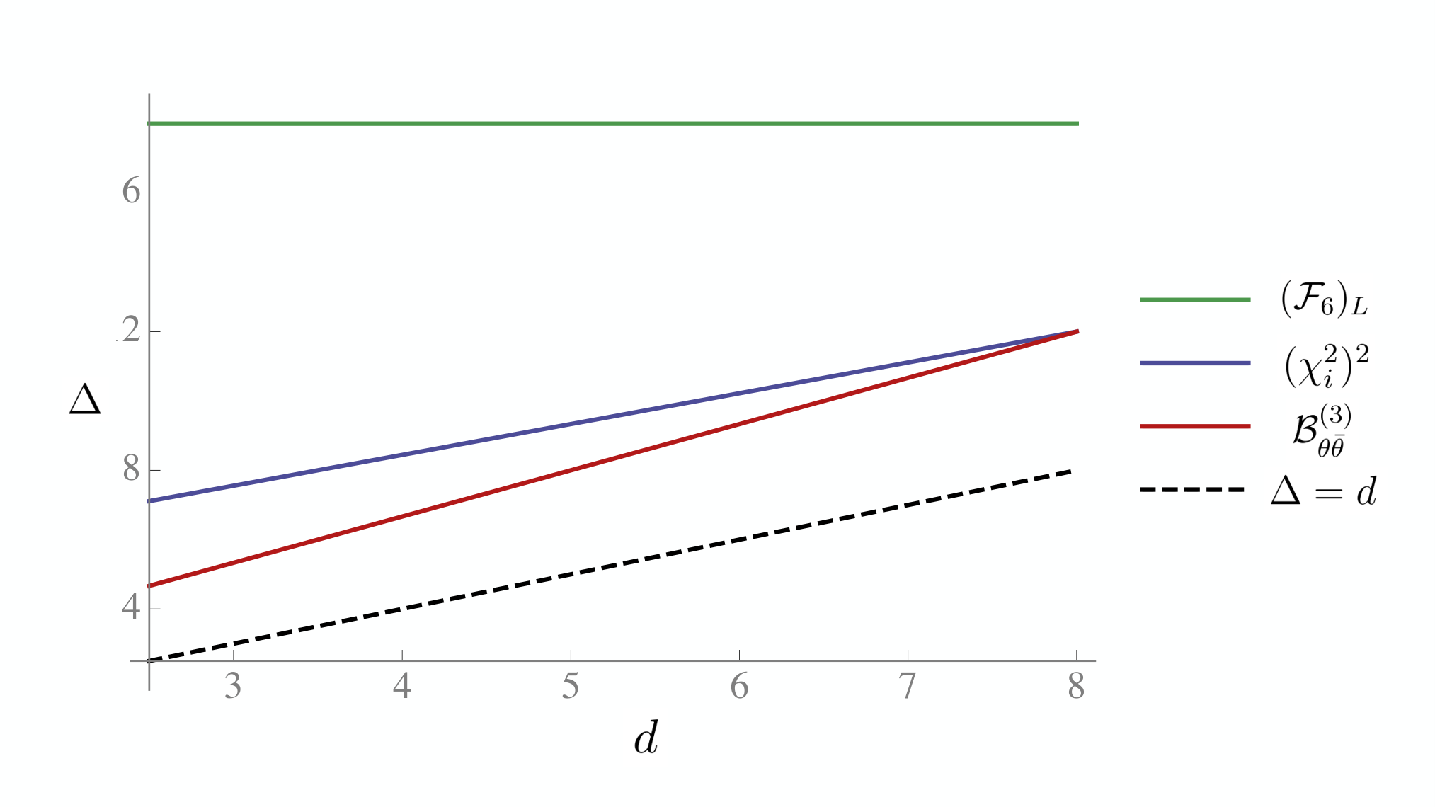
Comparing with the marginality line we see that none of the operators becomes relevant. Since we do not find any new relevant perturbation we can conclude that the SUSY fixed point persists even at and thus that the RF model always undergoes dimensional reduction.
Of course our conclusion has to be taken with a grain of salt. Besides the non-perturbative mixing (which should not significantly change our results), there is a more important source of uncertainty. Indeed our conclusion relies on a one-loop computation of the anomalous dimensions. Since we are extrapolating to , higher loop corrections may become important. It would be very interesting to compute them and see if our results are confirmed.1414 14 We checked that a Padé[1,1] approximation does not change our observation that none of the considered operators crosses marginality. However it would be nice include higher loop computations in the analysis. We leave this task for the future.
One of our main motivations for this work was to check if the RG setup introduced in [1] to study the RFIM model would give consistent results also for RF . Recall the discussion from section 1 that the RF model describes the near critical behavior of branched polymers. As first established in [17] according to numerical evidence, the critical point of branched polymers is related to the non-disordered Lee-Yang fixed point (which describes critical point of Ising model in an imaginary magnetic field) via dimensional reduction in all . Consequently it is expected that the critical RF model in this range of dimensions is always described by a supersymmetric fixed point. Our conclusion above is therefore consistent with this expectation (see the next section for a discussion on the subtle case).
Another motivation was to compare how the single RG setup works in different ways for RFIM and RF (see Fig.3). Indeed in [1] we found that for the RFIM the SUSY fixed point becomes unstable at a critical dimension - (namely for the fixed point is non supersymmetric). On the other hand we expected no instability for the RF . It was interesting for us to see how this would come about. This paper provides an answer to this puzzle. The main source of instability for the RFIM is due to (which we called in [1]) and . They are found to have vanishing one-loop anomalous dimension. The first non-vanishing contribution is found at two-loops and it is negative (see footnote 12). So the main difference is that in the RFIM their one-loop correction vanishes, leaving a leading two-loop negative correction. For the RF we did not compute the two-loop correction of and because their one-loop anomalous dimension is already positive and fairly large.1515 15 Still it would be interesting to compute the two-loop correction. One can easily understand why the one-loop corrections behave differently in the two models. Indeed these are computed in a different way: one needs to insert two interaction vertices to compute a one-loop correction in the RF while a single vertex is required in the RFIM (this is also true for the pure versions of the models and it is simply due to the fact that the vertices have odd or even number of fields). Operators made of only fields (like the Feldman operators) clearly do not receive corrections from the insertion of a single vertex since the latter always contains other fields (e.g. the vertex has extra powers of which cannot be contracted with the fields of the Feldman operator). Therefore by construction in the RFIM all Feldman operators have zero anomalous dimension at one loop, while for the RF this need not be the case and indeed we find that it is not. We thus conclude that by applying the single RG framework of [1] we obtain the expected results in two different models. This gives us more confidence that the framework of [1] is indeed correct.
5 Discussion
In this paper we carry out a perturbative RG analysis of the Random Field model. We use the framework introduced to study the Random Field Ising Model in [1].
The results of [1] are compatible with the numerical observations [5, 6, 7] that supersymmetry (and thus dimensional reduction) of the RFIM fixed point are lost in and are recovered in , where is the upper critical dimension. In [1] this is explained by the fact that (at least) one operator becomes relevant in dimensions where - . For the RF model the numerical expectation [17] is that the SUSY fixed point is always reached in (where is the upper critical dimension, while the subtle case is discussed below). The main result of this work is a check that the framework introduced in [1] is compatible with the numerical results. Indeed we studied a large number of low lying perturbations and we found that at one-loop they all have positive anomalous dimensions and they do not seem to ever cross the marginality line.
This result is important for two main reasons. Firstly it is a check of the RG framework of [1]. Indeed we gained more confidence that this framework is correct since gives results compatible with the RF expectations. Notice that it is crucial to test this framework since it provides a new understanding of when and why the RFIM undergoes dimensional reduction, which is a question which was debated for almost fifty years. Secondly it explains in the same language used for the RFIM why dimensional reduction is not lost for the RF itself. The latter is also an important question. Indeed the RF theory captures the phase transition of a number of interesting statistical physics models like branched polymers and lattice animals. For these models dimensional reduction was observed to hold giving rise to the Lee-Yang universality class in dimensions. Our calculations are in perfect agreement with these results.
Interestingly, for the problem of branched polymers Brydges and Imbrie proposed a model that has explicit Parisi-Sourlas supersymmetry at the microscopic level and which, by construction, undergoes dimensional reduction [18]. On one hand the result of Brydges and Imbrie is impressive because it explicitly shows how dimensional reduction works in the problem of branched polymers without even using field theory or RG. On the other hand [18] only shows dimensional reduction for a very fine tuned model where supersymmetry is taken as a starting point.
In particular in [18] it is missing an explanation of why supersymmetry should emerge in the IR for a generic non-supersymmetric model of branched polymers.1616
16
E.g. the model proposed in [18] is not sensitive to susy-null and non-susy-writable perturbations which were crucial to understand the destabilization of the SUSY fixed point in the RFIM. Our work provides an answer to this question by showing that all SUSY-breaking deformations are indeed irrelevant.
There are many open problems which deserve further investigation (see also the discussion section of [1]) and our work should be viewed as a first step in this direction. Some of the most interesting ones are listed below.
- 1.
Higher loops and other operators : All the anomalous dimensions computed in this paper are at one loop. It would be interesting to compute higher loop corrections of the low lying leader operators. This would allow one to verify that SUSY fixed point is indeed stable for larger values of . Susy-null and non-susy-writable leaders like and need to be studied in the theory. This is slightly more complicated than the usual theory (Lee-Yang) fixed point in , since the Lagrangian contains two interaction vertices and three different propagators. However using modern multi-loops technologies it should be fairly easy to extend the results of this work to higher orders in perturbation theory. For the susy-writable leaders like the box operators the computation can be directly done in the usual theory (because of dimensional reduction), by computing higher loop anomalous dimensions of the operators.
We also ignored other perturbations with higher classical dimensions, e.g. susy-null leaders not in the class and non-susy-writable leaders that are not of the form or of the Feldman type. It would be interesting to compute their anomalous dimensions. This may be useful in order to understand nonperturbative mixing when is large. It should be kept in mind that for operators with higher classical dimensions good accuracy is expected only at higher loops.
- 2.
Conformal Bootstrap : It would be interesting to set up a conformal bootstrap problem for the RF fixed point.1717 17 See [24] for an attempt by Hikami, reviewed in App.A.10 of [1]. This would be a strong check of the stability of the SUSY fixed point and dimensional reduction. Choosing a 4-point function appropriately one can shed light on the various operators allowed in the theory in the nonperturbative regime . E.g. non-susy-writable operators like can be exchanged in the conformal block decomposition of , so we could numerically estimate their dimensions by bootstrapping this correlator.
There are a number of challenges in setting up this bootstrap problem. Firstly, we do not have a CFT for positive integer values which we can analytically continue to . This is because the fixed point only exists at (the fixed point arises as the limit of a sequence of approximate fixed points as we review in section 2.1). Second, since we are working in an invariant theory with we expect to find a logarithmic CFT [25]. Indeed for the RFIM case we find logarithmic multiplets (see section 9.2 and app. H of [1]), and one should expect the same for the RF model. In order to account for logarithmic multiplets one needs to use a different bootstrap algorithm which makes use of logarithmic conformal blocks [26]. Finally the CFT is nonunitary as evident e.g. from the dimension of . So one cannot impose unitarity bounds or positivity of OPE coefficients. For nonunitary CFTs one needs to resort to Gliozzi’s bootstrap algorithm [27] or to variations thereof, which typically are less systematic. Some work is required to tackle these problems, but certainly it would be priceless to have at our disposal the bootstrap toolbox to study random field theories.
- 3.
Dimensional reduction : The RF model can also be studied in . In this case, according to dimensional reduction, one would obtain a relation to the pure theory in zero dimensions. This case is of course bound to be singular. E.g. dimensional reduction for correlation functions is obtained by localizing all operators to a dimensional hyperplane, however this prescription is not well defined for , since all insertions would collapse to a single point. On the other hand one can compute the partition function (and related observables) in the RF model for and relate them to the zero-dimensional counterpart, where the zero dimensional path integral is just understood as an ordinary integral. Parisi and Sourlas in [17] checked that critical exponents behave according to dimensional reduction even at . The problem was later reconsidered in [28], where it was suggested that the theory does not have the structure of a conformal theory. Indeed for the Parisi-Sourlas supersymmetric theory is of a subtle type since it is not clear if it can possess a traceless super-stress tensor. This problem can be explicitly seen in free theory by looking at formula (C.4) of [8] where the improvement term which makes the stress tensor traceless is singular for . We think that it would be worth to revisit this problem in a modern language to get a more comprehensive understanding of this two-dimensional theory and of its dimensional reduction.
- 4.
Dimensional reduction : A less singular case arises for the dimensional reduction . Here one can still consider correlation functions restricted to a line. On the other hand, again we cannot define a stress tensor in since all one-dimensional theories are non-local. This can be again seen in Parisi-Sourlas supersymmetric free theory where one finds that the dimensionally reduced stress tensor —see e.g. in (C.6) of [8]— vanishes. It would be interesting to study in more detail the three-dimensional SUSY theories and their dimensional reduction.
- 5.
Dimensional reduction : Finally we would like to mention that the dimensional reduction is not singular but it is very interesting. Indeed the dimensionally reduced models have emergent Virasoro symmetry (e.g. the RF theory in dimensionally reduces to the Yang-Lee minimal model with central charge ). It would be very interesting to investigate how the Virasoro symmetry is embedded in the supersymmetric theories. This direction deserves further investigation [29].
- 6.
Applications to other models : Beside RFIM and RF theory, there are other models which could be potentially studied in the RG framework used in this paper. Indeed in statistical physics one often uses the replica method and sometimes one lands on Lagrangians of the form (2.3) or generalizations thereof (see e.g. [30] for a model of the continuous phase transition of glassy materials). It would be interesting to further apply the RG framework of [1] to these cases both as a test of the method and to see whether it provides a deeper understanding of a broader class of phenomena.
Acknowledgements
We would like to thank the participants of the workshop “Bootstat 2021” which took place at Institut Pascal (Université Paris-Saclay) with the support of the program “Investissements d’avenir” ANR-11-IDEX-0003-01. We especially thank Silvio Franz for interesting discussions and Slava Rychkov for comments on the draft and collaboration in the early stages of the project. The work of A.K. is funded by the German Research Foundation DFG under Germany’s Excellence Strategy – EXC 2121 “Quantum Universe” – 390833306. The work of E.T. is supported by the European Research Council (ERC) under the European Union’s Horizon 2020 research and innovation programme (grant agreement No 852386).
Appendix A Review of branched polymers and lattice animals
In this appendix we review how to define the problem of diluted branched polymers/lattice animals and see why it is captured by the RF theory. We will follow the construction of [31] and we aim at giving a pedagogical and explicit definition of all the ingredients of the model (see also chapter 9 of [32]).
Let us start with some basic definitions. A polymer is defined as a linear chain of units called monomers. A branched polymer is built by sewing together linear polymers. It is convenient to define the polymers on a lattice so that for any fixed number of monomers, there is a finite number of configurations. We define a polymer on a dimensional hypercubic lattice by placing the monomers at the sites of the lattice and by connecting neighbouring sites with lines. Sets of connected sites on the lattice are called “lattice animals” or “clusters”. When lattice animals have a tree-like topology they define branched polymers. General lattice animals also contain self intersections (i.e. closed loops) as shown in figure 4.
We are interested in studying the statistics of branched polymers/lattice animals when the number of monomers is very large: in this limit the number of possible configurations and the average size of a cluster scale as and where are critical exponents, while is a non-universal constant. The models of branched polymers and lattice animals are known to be in the same universal class (see discussion below). In the following we define a model which counts configurations of lattice animals, which allows us to choose how many links, loops, clusters and vertices are present in a given configuration. Finally we will be interested in the so called diluted limit, which suppresses configurations with multiple clusters.
We will introduce the model in steps. We will start by defining a toy-model that is used to build random walks (which are equivalently understood as linear polymers). We then introduce vertices to allow for branching. Finally we explain how to modify the model to count the number of separate clusters. We conclude the appendix by showing that the IR behaviour of this model can be described in the continuum limit by an action with symmetry which is of the same form as the replica action of (2.3).
To start we consider a simple model with an -state vector with partition function
| (A.1) |
where denotes nearest neighbour sites. We want to consider to be variables in which are spatially uncorrelated with trace defined as
| (A.2) |
where is an invariant distribution. By invariance we must have that
| (A.3) |
and zero if is odd, for some coefficients . The dots in (A.3) represent products of Kronecker deltas for all possible inequivalent pairings of the indices . In order to build the model we further require the coefficients to satisfy the following conditions
| (A.4) |
where the coefficients must be finite in the limit . Finally we also need to be able to tune the coefficients to the values we want. Later we will explain why these conditions are useful.
These conditions can be recast as restrictions on the possible distributions . In other words it is possible to choose in such a way that all these conditions are satisfied. A simple way to do this is to choose a distribution written as a Gaussian times a polynomial in . This distribution gives rise to computable traces (by Wick contractions) and one can easily check that by tuning the coefficients of the polynomial one can fix the same number of coefficients .1818 18 To be explicit, given the distribution (A.5) one finds that , where are even integers. The linear map between with and with is invertible and we can therefore use it to fix this set of to any value by opportunely tuning the coefficients . This means that by considering it is possible to satisfy (A.4) and to even choose the values of .
Formula (A.1) corresponds to a Hamiltonian , which is a slight modification of the usual model due to the presence of the logarithm. This formulation gives a simpler partition function which has at most a single bond between two sites and thus it can be conveniently described diagrammatically in terms of clusters. Let us show how this is done. We first expand the product in (A.1) to get a sum of terms each of which is just a product of bonds for a given set of . This product is then depicted by drawing a line between each two sites if a bond between them is present. A cluster is thus a set of connected bonds. Now the important observation is that by tracing over the only clusters that survive are closed loops. Indeed for each open end we get . Moreover for each separate loop we get a factor of due to the sum over . There are also configurations with intersecting loops which arise when more than two spins are present at the same site. Forgetting about the latter (which we will discuss below), the partition function can be expressed as
| (A.6) |
where is a cluster configuration which only contains loops, counts the number of loops in and the number of bonds. Now we want to take the limit . This has two important consequences: first it suppresses loop configurations, secondly because of (A.3) it suppresses traces of more than two spins at a given vertex, thus eliminating all configurations with intersecting loops and leaving only linear configurations. E.g. at order the limit selects only configurations with a unique self avoiding loop. While this limit trivializes the partition function, it is typically used to study two point functions of a spin variable
| (A.7) |
By expanding again the product we notice that presence of makes it possible to draw new diagrams which are lines that connect to . These configurations are not suppressed by the limit because the operator is selecting a single component of the possible . In practice all configurations are written in terms of lines that connect at different sites (all the other spin components are not present in any configuration). Conversely, choosing the two point function of would have generated an extra factor of for the lines due to the sum over . Equation (A.7) is used to compute the statistics of self avoiding walks between two points.
For the problems of branched polymers and lattice animals we want to sew together many self avoiding walks. A first step to do so is to allow many endpoints, namely we can multiply the partition function (A.1) by a term . This is not enough since as it would only generate configurations involving a number of linear self avoiding walks weighted by . In order to obtain branched configurations we need to introduce vertices which allow us to connect lines to the site . These can be defined by the requirement
| (A.8) |
where if all are equal, otherwise it is zero. Since the index of counts how many lines are attached to a given site, for a hypercubic lattice we need only to build a finite number of vertices with . Also the label is restricted by the possible number of spins at a given site in the nearest neighbour interaction (A.1), which gives . The operators are written in terms of the spin variable . We ask to preserve the symmetry that rotates the variables with . In practice we can define as a polynomial of order in the spin variables which depends on and . Let us exemplify this by considering the simplest vertex for . We start by the ansatz for some coefficients .1919 19 We did not include even powers of the spin variable because (A.8) gives rise to an independent set of linear equations for the correspondent coefficients which is homogeneous and thus has trivial solution, namely we can set all these coefficient to zero. The coefficients of the ansatz are fixed by requiring that (A.8) is satisfied for . Notice that from these two requirements we obtain three equations which arise from the different tensor structures. E.g. from we get a single equation that multiplies which we want to set to zero. From we get two equations. One from the coefficient of which we want to set to zero and one from the coefficient of which we want to set to one. In particular using (A.3) and (A.4) we can solve the full set of equations obtaining
| (A.9) |
By simple power counting this automatically satisfies (A.8) for all because of the scaling in of (A.4).
This example not only shows how to construct the vertices but also it clarifies why we need to be able to tune the coefficient . Indeed we must ask that the denominators of the equations above are not vanishing, namely and .2020 20 E.g. these requirements are not satisfied by the distribution which gives and thus . In other words, the existence of vertices with the property (A.8) is an extra requirement which is not trivially satisfied by all distributions . We can go on by repeating this construction for vertices with higher . The number of coefficients in the ansatz for the vertices matches the number of independent tensor structures appearing in the equations (A.8) for (this is ensured by symmetry) and thus we are able to fix all the coefficients in terms of the variable . We checked this algorithm and found explicit formulae for the vertices for . We do not report the results here since the expressions are lengthy.
Using the vertices we can write a new expression for the partition function
| (A.10) |
where the coefficients are introduced to count the number of vertices with lines in a configuration. It is important to notice that for a given site we can either have a simple point, an endpoint or a vertex . This means that we never have to consider traces of two vertices and and therefore that (A.8) is enough to compute all possible configurations. It is also worth mentioning that in this model there cannot be more than spin variables at a given site (this happens when a vertex is attached to lines) which explains why we required the maximal value of in the conditions (A.4) to take this value.
Because of the vertices, the partition function now also generates loop configurations (thus generic lattice animals and not only branched polymers) as long as they are constructed by connecting and endpoints. E.g. the simplest loop configuration is obtained by attaching an endpoint to one of the lines of a vertex and by making a closed loop with the remaining two lines — giving a weight . This term will not scale as because all the spin variables in the diagram must be of the form .
A problem of this model is that it does not give us any handle to count the number of separated clusters. E.g. a diagram weighted by (see figure 5) could either be a vertex attached to three open ends or it could be made of two separate clusters, the first being like the one described above with weight and the second one being a line that connects two points with weight .
This is not what we wanted, since we aimed at counting the number of configurations of a single lattice animal. In the following we explain how to modify the model in order to count the clusters. This will be crucial to take the dilute limit in which configurations with multiple clusters are suppressed.
There is a very simple way to count clusters. Indeed, as mentioned above, a linear cluster obtained by inserting at the open ends the operator (instead of ) is weighted by a factor of (similarly the weight of is kept for branched clusters if one uses vertices that satisfy instead of (A.8)). Here however we do not want to use to count the number of clusters, since this variable is already used to count the number of loops. The idea is thus to introduce a new index in the spin variable obtaining with and , where the new parameter will be used to count clusters. The label is independent of but works in a very similar way. The trace is defined as
| (A.11) |
where is an invariant distribution which thus gives
| (A.12) |
and vanishes when is odd. The dots contain products of Kronecker deltas for all pairings of the indices —such that every always appears multiplied by with the same . We require the coefficients to satisfy the conditions
| (A.13) |
where again we want to be able to tune the values of which must be finite in the limit . As before all these conditions can be met by considering as a Gaussian distribution multiplied by a polynomial with opportunely chosen coefficients.
We thus define the partition function
| (A.14) |
where the new vertex satisfies
| (A.15) |
for and . The vertices are built as polynomials of order in the spin variable which preserved symmetry and whose terms are assembled from the building blocks and . It is easy to see that the same ideas used to construct can be generalized to define the vertices . E.g. a vertex that satisfies (A.15) can be defined as follows
| (A.16) |
with
| (A.17) |
As before the coefficients are tuned to avoid singularities.
By expanding the partition function in the limit we obtain
| (A.18) |
where is a configuration that contains bonds, endpoints, separated clusters and vertices with legs. The presence of all these parameters allows us to count the number of loops in a given configuration, which is obtained through the relation . We thus obtain a partition function of the form
| (A.19) |
where
| (A.20) |
We further want to consider the diluted limit, namely the case in which there are few clusters. To do so we take the limit . The resulting partition function generates lattice animals; in principle one could get branching polymers by forcing the number of loops to zero by taking (or equivalently ) in (A.19) while keeping the rest of the ’s finite. We avoid this procedure and keep finite since lattice animals and branched polymers are known to be in the same universality class. While there is no full proof of the latter statement, this was checked in various numerical works (see e.g. [33]) and also at low order in perturbation theory in [31]. Given the formulation (A.14), the fact the two models are in the same universality class can be rephrased by saying that the RG flows which start at infinite or finite in the UV should end up in the same IR fixed point. As a final comment, we would like to mention that in physical systems where branched polymers arise one cannot typically exclude the presence of closed loops [34] so in fact lattice animals define themselves a physically relevant system.
Now that we constructed the model (A.14) which counts diluted lattice animals, we want to show how to reformulate it in terms of a field theory. We start by rewriting the partition function as follows
| (A.21) |
where the Hamiltonian takes the form
| (A.22) | ||||
The model has a continuous symmetry which rotates the components of . This arises because the original symmetry is broken by the end points and vertices which are built in terms of powers of spins in the direction . The symmetry is not going to play any role in the final field theory since the directions are not going to be critical. This may not be so counterintuitive since also in the cluster representation only the spin was contributing to the configurations. There is an extra symmetry which acts by permuting the components . This arises because the vertices contain powers of with arbitrary . We thus expect to obtain a model in the continuum limit which has symmetry in the limit . In the following we shall explain how this arises in more detail.
We first consider the nearest neighbour interaction term of (A.22). Each term in the expansion of the logarithm can be further Taylor expanded for small lattice spacing between neighbouring sites. The result is written as a polynomial in dressed with derivatives. E.g. let us consider the term in the expansion of the logarithm and let us work for simplicity in ; in this case a site has two nearest neighbours at position and , so . Similarly the term give rise to and so on. Of course it is trivial to generalize this to higher dimensions by using derivatives along all space directions. The terms in the second sum in (A.22) are defined at a single site so they do not change by taking the continuum limit (however we still have to include in the final action all possible terms in the expansion of the logarithm). The result takes the form
| (A.23) | ||||
where the first dots correspond to terms with higher powers of possibly dressed with derivatives and the second dots take into account higher powers of which multiply . The coefficients are written in terms of and the lattice spacing while the coefficients are written in terms of polynomials in the variables and . In order to have an action written in a canonical form we first to rescale the fields to get a kinetic term normalized as . Secondly we get rid of linear terms proportional to in the action by shifting . Because of this shift, the coefficients multiplying the monomials in and in become different. In particular the mass terms and appear with a different coefficient. When we study this action in the IR we tune the mass for in order to reach the critical point. All other fields are massive and are integrated out. The resulting action takes the form of an model
| (A.24) |
where the dots stand for any invariant interaction defined by powers of possibly dressed with derivatives and the coefficients are written in terms of the and of (A.23). After mapping , this action is exactly of the form (2.3) (with and ) which is the starting point for analyzing the RF model in terms of replica variables.2121 21 Notice that in the dots of (A.24) there is also the term . This term corresponds to what we call in the main text, which is an irrelevant deformation.
Appendix B Classification of leaders in RF theory
The classification of leaders of the RF theory is very similar to the one of the RFIM described in [1]. Indeed, the form of the leaders does not depend on the potential , nor on the space dimensions. The only differences are the following. First the classical dimensions of the fields depend on the spacetime dimension and the latter is different in the two models (since we work close to the respective upper critical dimension). Secondly the RFIM has an extra symmetry, and thus one is allowed to focus on leaders which are singlet under (which are all composite operators made out of an even number of elementary fields). In the RF theory the symmetry is absent, we will thus need to consider also operators made out of an odd number of elementary fields.
Let us call the number of elementary fields and the number of derivatives that are contained in the composite operators. As an example of even- leaders, let us consider the case of . As for the RFIM, the possible singlets without derivatives are , . All leaders with must be susy-writable as it was discussed in [1]. Here the only difference is that their dimensions is computed in , as shown in table 2.
| Singlet | Leader | Leader type |
|---|---|---|
| susy-writable | ||
| susy-writable |
Similarly operators with derivatives will have the same exact form as the one described in [1]. E.g. . This should make it clear that we do not need to repeat the classification for all even , which is given in [1] and still holds, up to the scaling dimension of the fields which can be very easily recomputed following the rules that , and . It is easy to see that this amounts to shift the dimension in all tables of [1] by , namely
| (B.1) |
Applying the equation above to the cases studied in [1] we find the lowest dimensional leaders in the even- spectrum of theory in : the first susy-null leader is with dimension while the first non-susy-writable leader is and only appears at dimension . In [1] other susy-null leaders appear at , the second one is with dimension in . In the following we want to check if in the odd- spectrum of theory there are new low lying leaders in the susy-null and non-susy-writable sectors. We will see that there are no new non-susy-writable leaders at , therefore the lowest dimensional leader of this type is still .2222 22 Another non-susy-writable leader is and can be found at dimension as explained in the main text. In this appendix we will not show this leader because we decided to focus on . Similarly we find that the first susy-null leader is still , however we also find other susy-null leaders at with odd . The first new one is which appears at and has dimension in . In equation (3.9) in the main text we show that this operator is a member of an infinite class of susy-null operators named , which have leaders equal to , which also describe the cases and discussed above.
B.1
A single operator with is present,
| (B.2) |
which is susy-writable. When we add this operator to the Lagrangian, the physics does not change since can be reabsorbed by shifting the fields. In SUSY language it corresponds to adding to the SUSY Lagrangian. Equivalently this corresponds to adding to the dimensionally reduced Lagrangian. In both cases this perturbation can simply be undone by a shift in the fields (respectively and ).
B.2
There are only three leaders with and no derivatives. They are all of the susy-writable type as shown in table 3.
| Singlet | Leader | Leader type |
|---|---|---|
| susy-writable | ||
| susy-writable | ||
| susy-writable |
We can also consider leaders with and two derivatives. The result is still a list of susy-writable operators as shown in table 4.
| Singlet | Leader | Leader type |
|---|---|---|
| susy-writable | ||
| susy-writable | ||
| susy-writable | ||
| susy-writable |
By increasing the number of derivatives we do not find new interesting operators. Indeed all with have a susy writable leader with no followers. So, any combination of these with any number of derivatives will be susy-writable. One can thus focus on —which is the only operator with that has followers (which are not always susy-writable)--- and try to dress it with derivatives. But one can see that these do not produce new non-susy-writable or susy-null operators. Indeed we first notice that there exists a single independent2323 23 All other dressings are equal to plus total derivatives plus terms built by dressing and with derivatives (which we already considered above). way to write a Lorentz scalar by dressing with derivatives: . The associated leaders are susy-writable. One may still worry that another singlet could have the same susy-writable leader and that their difference should be considered as a new leader. However the leader of has lower dimension than any other leader built by composing products of and dressed by derivatives, as one can see for the example of two derivatives in table 4. This ensures that there is no other singlet with the same leader and therefore that the followers of can always be neglected. In summary we find that no matter how many derivatives we consider, any operator built out of fields must have a susy-writable leader.
B.3
We now focus on the operators built out of five fields. The list of leaders with and is shown in table 5. Here we find the first odd- susy-null operator which we call according to the definition (3.9) in the main text. This operator has dimension and leader equal to . At dimensions we also find the new susy-null leader .
| Singlet | Leader | Leader type |
|---|---|---|
| susy-writable | ||
| susy-writable | ||
| susy-null | ||
| susy-writable | ||
| susy-null | ||
| susy-writable |
By considering we must take into account the following singlets
| (B.3) | ||||
Combinations of these singlets give either susy-writable or susy-null leaders. At dimension there are five leaders: three susy-writable and two susy-null. Since the two susy-null leaders have dimension greater than , they are not very important for our classification. However it is instructive to show their explicit form:
| (B.4) | ||||
| (B.5) |
which gives rise to the susy-null leaders
| (B.6) |
It is interesting to notice that the leaders of and are just total derivatives, indeed these operators can be written as derivative of spin-one -singlets,
| (B.7) | ||||
| (B.8) |
Since the operators are total derivatives they do not affect the RG and we can discard them for the purpose of the present classification. Analogous considerations are valid for the next null operators with which have dimensions and are built by dressing with derivatives.
By studying higher number of derivatives with we do not find any non-susy-writable leader with . E.g. by considering the lowest dimensional operator is dressed by derivatives which has a susy-writable leader with dimension , while the first susy-null operator has already dimensions .
To summarize for we found that the lowest dimensional susy-null leader is and that there are no non-susy-writable leaders up to .
B.4
The leaders with and are considered in table 6 We notice that the only susy-null operator belongs to the family for and it has dimension in .
| Singlet | Leader | Leader type |
|---|---|---|
| susy-writable | ||
| susy-writable | ||
| susy-null |
It is easy to see that all leaders with and are susy-writable.
Appendix C Box operators
The only susy-writable operators which may destabilize the SUSY fixed point are those which transform in the irrep of OSp. Since these are susy-writable their anomalous dimensions are determined by computing anomalous dimensions of the corresponding operators in theory in dimensions. In this appendix we show the form of these operators both in theory and in the SUSY theory.
In order to define operators which have good scaling dimension at one loop, we consider the primary operator built out of free scalars in dimension. We are interested in primaries that transform in the representation of . It is easy to show that they take the form
| (C.1) |
where . To unpack (C.1), we contract it with polarization vectors such that . We thus obtain
| (C.2) | ||||
where each derivative is meant to act only on the closest on its right. The two lowest dimensional operators of this family are thus and .2424 24 To study the RFIM in [1] we considered the operator , since it is the lowest dimensional operator in this representation which is -even. Here the symmetry is not present thus we are allowed to consider operators built out of an odd number of elementary fields like .
We now want to write down the correspondent SUSY superprimary . We are especially interested in the highest component with all indices in directions and . The operator was explicitly written in [1] (in ). In the following we thus focus on , which can be written in components as follows
| (C.3) | ||||
where here, for simplicity, we set . To compute anomalous dimensions of this operator, one can alternatively consider the lowest component of the same supermultiplet, which has a considerably simpler form
| (C.4) |
In App. D.3.4 we will compute the anomalous dimensions of using the formulation (C.2) in terms of the theory. It would be nice to check this computation using the SUSY descriptions (C.3) or (C.4).
Appendix D RG computations
In this appendix we give the details of the results shown in section 3. All our computations will be at one loop order. For our theory this typically involves two vertices. It is suitable to use Feynman diagrams for such cases, as opposed to the OPE method we used for one-loop computations in [1]. We will use dimensional regularization scheme in our computations for which we refer to [21, 35] for a good review.
We will work with the fields instead of fields. This is suitable for computing anomalous dimensions of general susy-writable, susy-null and non-susy-writable operators.
D.1 Wavefunction renormalization
Our theory is given by the Lagrangian (2.20) in dimension, written in Cardy variables and mass term set to zero:
| (D.1) |
The subscript ‘’ denotes bare quantities that are related to the renormalized ones as follows: 2525 25 Although we could consider separate renormalizations for the couplings corresponding to and , it is sufficient to focus on just one. We comment later that the two vertices lead to the same renormalization constant and beta function.
| (D.2) |
Here is an arbitrary mass scale. The -s denote renormalization constants which can be expanded in powers of and as follows:
| (D.3) |
where the subscript . The above is very much similar to the usual -theory fixed point in dimension. Correlation functions of the bare quantities contain poles. Since those of the renormalized ones must be finite we should choose accordingly.
We begin with the most basic computation which is to obtain the wavefunction renormalization constants . For this we consider the correlators , and and demand that they should be finite. Their corrections are shown in Fig. 6 and 7. The corrections to and are equal and given by the integral:
| (D.4) |
The correction to contains the above and also the additional integral :
| (D.5) |

Taking into account the respective symmetry factors the one-loop corrected 2-point functions are given by :
| (D.6) | |||||
This leads to
| (D.7) |
D.2 Beta function
We will now compute the one-loop beta function. For this we consider the 3-point function and demand that it is free of poles. The tree level diagram involves the vertex. The one-loop diagrams are of the type shown in Figure 8 . The amputated form of the 3-point function is given by:
| (D.8) |
The renormalization constants appear through via (D.2). is given by the integral
| (D.9) |
This is a triangular loop integral that can be evaluated using standard methods (see e.g. [21, 35]) , and gives the following pole:
| (D.10) |

Demanding that the pole cancels, and using the wave function renormalization constants from (D.7) we obtain
| (D.11) |
We thus obtain the beta function as follows:
This gives a fixed point at
| (D.12) |
The two solutions to are equivalent as they are related by transforming , .
D.3 Renormalization of local operators
For RG analysis of local operators we consider bare operators (composed of bare fields), that are related to renormalized operators by a mixing (renormalization) matrix :
| (D.13) |
Similar to the renormalization constants of previous subsection, the matrix can be expanded in powers of and as follows
| (D.14) |
The matrix has to be fixed by computing one-loop corrections to correlation functions of and requiring them to be free of poles. In general, this matrix is of block diagonal form. A certain block in corresponds to operators with equal number of fields and equal classical dimension .
The matrix gives the anomalous dimension matrix as follows:
| (D.15) |
Writing and using the definition of beta function it is then simple to obtain:
| (D.16) |
This has to be evaluated at the fixed point given by (D.12).
Diagonalization of gives the renormalized operators, whose dimensions are given by the eigenvalues. For an eigenvector satisfying , we get a renormalized operator having an anomalous dimension .
D.3.1 Anomalous dimension of
Let us first compute the anomalous dimension of the fundamental fields . Their renormalization constants we computed in (D.7) . Using (D.16) we immediately get the anomalous dimension:
| (D.17) |
As expected this is same as the well-known field anomalous dimension for Lee-Yang fixed point in dimensions [21].
D.3.2 Susy-null leaders
In this section we will compute the anomalous dimensions of some susy-null leader operators. The ones we consider correspond to the class of singlet operators we introduced in section 3.2. For their leaders give susy-null operators with the three lowest classical dimensions. These are given by respectively. Since each has the lowest classical dimension among operators with fields we may simply represent their respective renormalization constants as follows:
To compute the renormalization constant we consider the correlator
The one-loop triangle diagram corrections are shown in Figure 9. All the diagrams involve the same loop integral that we had earlier in (D.9).

It is straghtforward to compute the symmetry factors associated to each diagram. Demanding that the term vanishes from the correlator above we get the following condition:
| (D.18) |
Here is to account for external leg corrections and is given by (D.4). With computed previously in (D.10) we get the following condition for cancellation of singlarities:
D.3.3 Non-susy-writable leaders
Next we consider non-susy-wriable leader operators. We will focus on leaders of the particular class of singlets, call Feldman operators. We defined them in equation (3.13) which we repeat for convenience:
| (D.21) |
To compute the anomalous dimension of this we should, in principle, consider all opoerators with fields and the same classical dimension as . Let us write their renormalization matrix as . We take . We then have a renormalization matrix that has the following form:
| (D.22) |
To show this consider the correlator . It has a one loop correction as shown in Figure 10. From the - legs and the associated contractions of matrices it is clear that we only get a correction to and no other component . The fact that the components () would be 0 was argued in app H.3 of [1], and this also applies for the cubic interactions considered in this paper. Hence for computation of anomalous dimension of we have only to compute the renormalization constant and can neglect the other operators .
D.3.4 Susy-writable leaders
In this section we will compute the anomalous dimension of a class of susy-writable leaders, specifically the box operators discussed in section 3.1 and App. C. For convenience we will compute anomalous dimension of the box operator in the theory in dimension. Via dimensional reduction that should give the same anomalous dimenision as the operator we want.
The theory has the Lagrangian shown in (2.28) which we rewrite below for convenience (here we canonically normalize the action since the anomalous dimensions are independent of this normalization):
| (D.26) |
The arguments are similar to what we described above in section D.3. The standard details of this theory (beta function, critical point value) are given in section 2.
We want to use a form of the box operator that is simple for computation. In [1] App. F we used the idea of equivalence class which contains an operator and other operators that are related to it by a total derivative. Hence all operators in are equivalent for perturbative RG computations. The box operator equivalence class has the following operator:
| (D.27) |
which we defined as for this section. It is easy to show that this is related to the form (C.2) by a total derivative.
We define its renormalization as follows:
| (D.28) |
We consider the correlator for computing . It can be shown that the box operator as shown in (C.1) is a primary in free theory. Therefore for computing the one-loop anomalous dimension we can ignore mixing with other operators.
We will focus on the case . The operator may be written as follows:
| (D.29) |
At tree level the correlator is proportional to:
| (D.30) |
The correction to the correlator is given by the triangle diagram as shown in Figure 11.

Then we have integrals of the following forms depending on which leg(s) the derivatives act:
where the indices have to be chosen as appropriate.
Let us focus on to show how to evaluate these integrals. We may write the denominator in as
| (D.31) |
Now using the standard change of variable the above becomes
| (D.32) |
From the numerator of one gets:
| (D.33) | |||||
The gives a term proportional to upon integration. Since the multiplicative factors of and tensors in (D.29) eliminates all traces, we can ignore it. The terms proportional to or are also simultaneously zero. So we are left with the last term of (D.33) which gives:
| (D.34) |
The integral is obtained by simply replacing . The is slightly more tedious as it is quartic in the numerator. But it follows exactly the same method, and gives:
| (D.35) |
The final answer should be written in a form that matches the tree level momentum dependence (D.30). The result from the loop integral can be brought to this form by using momentum conservation .
Demanding that the correlator is free of poles allows us to compute as follows:
| (D.36) |
The last part is the standard theory correction to the 3 external legs (see [21]). This gives the following anomalous dimension of :
| (D.37) |
Now let us discuss the case of for . The steps are similar to above. But there is one extra loop integral where the derivatives of are not distributed over the internal legs. It is given by:
| (D.38) |
We explicitly computed the anomalous dimension of for . By extrapolation we expect the result for generic to be given by
| (D.39) |
References
- [1] A. Kaviraj, S. Rychkov, and E. Trevisani, “Random field Ising model and Parisi-Sourlas supersymmetry. Part II. Renormalization group,” JHEP 03 (2021) 219, arXiv:2009.10087 [cond-mat.stat-mech].
- [2] A. Kaviraj, S. Rychkov, and E. Trevisani, “The fate of Parisi-Sourlas supersymmetry in Random Field models,” arXiv:2112.06942 [cond-mat.stat-mech].
- [3] A. Aharony, Y. Imry, and S. K. Ma, “Lowering of Dimensionality in Phase Transitions with Random Fields,” Phys. Rev. Lett. 37 (1976) 1364–1367.
- [4] G. Parisi and N. Sourlas, “Random Magnetic Fields, Supersymmetry and Negative Dimensions,” Phys. Rev. Lett. 43 (1979) 744.
- [5] N. G. Fytas, V. Martin-Mayor, M. Picco, and N. Sourlas, “Restoration of dimensional reduction in the random-field Ising model at five dimensions,” Phys. Rev. E 95 (2017) 042117, arXiv:1612.06156 [cond-mat.dis-nn].
- [6] N. G. Fytas, V. Martin-Mayor, G. Parisi, M. Picco, and N. Sourlas, “Evidence for Supersymmetry in the Random-Field Ising Model at ,” Phys. Rev. Lett. 122 (2019) 240603, arXiv:1901.08473 [cond-mat.stat-mech].
- [7] N. G. Fytas, V. Martin-Mayor, M. Picco, and N. Sourlas, “Phase Transitions in Disordered Systems: The Example of the Random-Field Ising Model in Four Dimensions,” Phys. Rev. Lett. 116 (2016) 227201, arXiv:1605.05072 [cond-mat.dis-nn].
- [8] A. Kaviraj, S. Rychkov, and E. Trevisani, “Random Field Ising Model and Parisi-Sourlas supersymmetry. Part I. Supersymmetric CFT,” JHEP 04 (2020) 090, arXiv:1912.01617 [hep-th].
- [9] J. L. Cardy, “Nonperturbative aspects of supersymmetry in statistical mechanics,” Physica D: Nonlinear Phenomena 15 no. 1, (1985) 123 – 128.
- [10] C. N. Yang and T. D. Lee, “Statistical theory of equations of state and phase transitions. i. theory of condensation,” Phys. Rev. 87 (Aug, 1952) 404–409. https://link.aps.org/doi/10.1103/PhysRev.87.404.
- [11] T. D. Lee and C. N. Yang, “Statistical theory of equations of state and phase transitions. ii. lattice gas and ising model,” Phys. Rev. 87 (Aug, 1952) 410–419. https://link.aps.org/doi/10.1103/PhysRev.87.410.
- [12] M. E. Fisher, “Yang-lee edge singularity and field theory,” Phys. Rev. Lett. 40 (Jun, 1978) 1610–1613. https://link.aps.org/doi/10.1103/PhysRevLett.40.1610.
- [13] J. L. Cardy, “Conformal invariance and the yang-lee edge singularity in two dimensions,” Phys. Rev. Lett. 54 (Apr, 1985) 1354–1356. https://link.aps.org/doi/10.1103/PhysRevLett.54.1354.
- [14] D. S. Gaunt, “The critical dimension for lattice animals,” Journal of Physics A: Mathematical and General 13 no. 4, (Apr, 1980) L97–L101.
- [15] S. Redner, “Mean end-to-end distance of branched polymers,” Journal of Physics A: Mathematical and General 12 no. 9, (Sep, 1979) L239–L244.
- [16] T. C. Lubensky and J. Isaacson, “Statistics of lattice animals and dilute branched polymers,” Phys. Rev. A 20 (1979) 2130–2146.
- [17] G. Parisi and N. Sourlas, “Critical Behavior of Branched Polymers and the Lee-Yang Edge Singularity,” Phys. Rev. Lett. 46 (1981) 871–874.
- [18] D. C. Brydges and J. Z. Imbrie, “Branched polymers and dimensional reduction.,” Ann. Math. 158 no. 3, (2003) 1019–1039, arXiv:math-ph/0107005.
- [19] J. Cardy, “Lecture on Branched Polymers and Dimensional Reduction,” arXiv:cond-mat/0302495 [cond-mat].
- [20] F. Wegner, Supermathematics and its Applications in Statistical Physics: Grassmann Variables and the Method of Supersymmetry, vol. 920. Springer, 2016.
- [21] M. Srednicki, Quantum Field Theory. Cambridge University Press, 2007.
- [22] F. J. Wegner, “The Critical State, General Aspects,” in 12th School of Modern Physics on Phase Transitions and Critical Phenomena. 1976.
- [23] D. E. Feldman, “Critical Exponents of the Random-Field Model,” Phys. Rev. Lett. 88 (2002) 177202, arXiv:cond-mat/0010012 [cond-mat.dis-nn].
- [24] S. Hikami, “Conformal Bootstrap Analysis for Single and Branched Polymers,” PTEP 2018 no. 12, (2018) 123I01, arXiv:1708.03072 [hep-th].
- [25] J. Cardy, “Logarithmic conformal field theories as limits of ordinary CFTs and some physical applications,” J. Phys. A46 (2013) 494001, arXiv:1302.4279 [cond-mat.stat-mech].
- [26] M. Hogervorst, M. Paulos, and A. Vichi, “The ABC (in any D) of Logarithmic CFT,” JHEP 10 (2017) 201, arXiv:1605.03959 [hep-th].
- [27] F. Gliozzi, “More constraining conformal bootstrap,” Phys. Rev. Lett. 111 (2013) 161602, arXiv:1307.3111 [hep-th].
- [28] J. D. Miller and K. De’Bell, “Randomly branched polymers and conformal invariance,” arXiv:hep-th/9211127.
- [29] E. Trevisani, “work in progress,”.
- [30] S. Franz, G. Parisi, and F. Ricci-Tersenghi, “Glassy critical points and the random field ising model,” Journal of Statistical Mechanics: Theory and Experiment 2013 no. 02, (Feb, 2013) L02001. http://dx.doi.org/10.1088/1742-5468/2013/02/L02001.
- [31] T. C. Lubensky and J. Isaacson, “Statistics of lattice animals and dilute branched polymers,” Phys. Rev. A 20 (Nov, 1979) 2130–2146. https://link.aps.org/doi/10.1103/PhysRevA.20.2130.
- [32] J. L. Cardy, Scaling and renormalization in statistical physics. Cambridge, UK: Univ. Pr., 238 p., 1996.
- [33] H.-P. Hsu, W. Nadler, and P. Grassberger, “Simulations of lattice animals and trees,” Journal of Physics A: Mathematical and General 38 no. 4, (Jan, 2005) 775–806. http://dx.doi.org/10.1088/0305-4470/38/4/001.
- [34] T. C. Lubensky and J. Isaacson, “Field theory for the statistics of branched polymers, gelation, and vulcanization,” Phys. Rev. Lett. 41 (Sep, 1978) 829–832. https://link.aps.org/doi/10.1103/PhysRevLett.41.829.
- [35] H. Kleinert and V. Schulte-Frohlinde, Critical properties of theories. World Scientiic, 2001.