ruledlabelfont=normalfont,labelsep=colon,strut=off
StructToken : Rethinking Semantic Segmentation with Structural Prior
Abstract
In previous deep-learning-based methods, semantic segmentation has been regarded as a static or dynamic per-pixel classification task, i.e., classify each pixel representation to a specific category. However, these methods only focus on learning better pixel representations or classification kernels while ignoring the structural information of objects, which is critical to human decision-making mechanism. In this paper, we present a new paradigm for semantic segmentation, named structure-aware extraction. Specifically, it generates the segmentation results via the interactions between a set of learned structure tokens and the image feature, which aims to progressively extract the structural information of each category from the feature. Extensive experiments show that our StructToken outperforms the state-of-the-art on three widely-used benchmarks, including ADE20K, Cityscapes, and COCO-Stuff-10K.
Index Terms:
Semantic Segmentation, Transformer.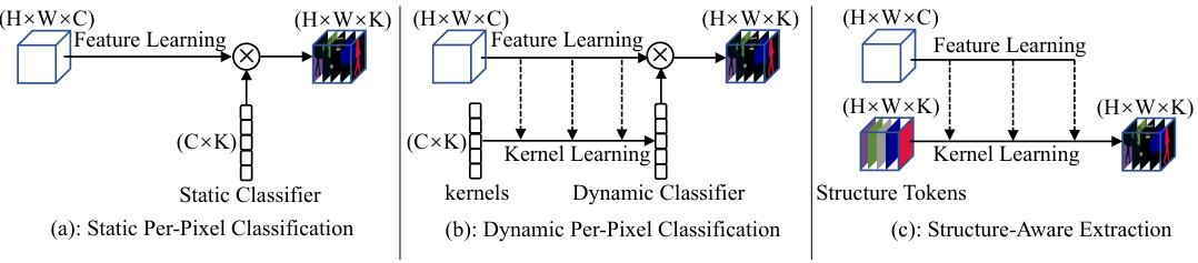
I Introduction
With the development of self-driving technology [16], human-computer interaction [18], and augmented reality [1], semantic segmentation has attracted more and more attention.
Since the deep-learning era, semantic segmentation has been mainly formulated as a per-pixel classification task, that is, classifying each pixel to a specific category via a learned classifier (such as a 11 convolution). According to the property of classifier, previous works can be categorized as two paradigms: static per-pixel classification and dynamic per-pixel classification. As shown in Figure 1a, for the static per-pixel classification paradigm, the classifier is fixed after the training process. The methods following this paradigm mainly focused on how to learn better representation for each pixel through context modeling [53, 7, 28, 45, 49] or automatic architecture design [47, 41, 11]. As the static classifier learned from the dataset can be regarded as a comprehensive representation of each class, which may not be consistent with the representation of each object in every image, some recent works [38, 10, 9] proposed to dynamically learn a classifier for different inputs according to their own contents. As shown in Figure 1b, the initial kernel is updated by the image feature, resulting in a dynamic classifier more adaptive to the current input.
In these two paradigms, the entire decoder is dedicated to learning better features (including precise semantics and details) and a more robust classifier, and the segmentation decision is only performed in the final segmentation head via the per-pixel classification. However, from the human perspective, the decision-making process of semantic segmentation presents a different pattern. In particular, based on the underlying knowledge of category-wise structural information (such as texture, shape and spatial layout), human beings first determine the rough area of each category and then gradually refine it, rather than paying close attention to all the image information at first and final performing the classification at one time. This motivates us to explore whether a paradigm more in line with the human decision-making process is better than the previously popular per-pixel classification for semantic segmentation.
In this paper, we design a human-like paradigm for semantic segmentation, named structure-aware extraction. To simulate human knowledge, we define a set of learnable structure tokens, each of which is expected to model the implicit structural information of one category. As shown in Figure 1c, given the image feature, the structure tokens gradually extract information from the image feature. Qualitative visualization shows that the structural information becomes more and more explicit during progressive extraction. Thus, the refined structure tokens of the final layer can be directly regarded as the segmentation result. Obviously, our paradigm is similar to the human-like process that uses structural knowledge to make rough discrimination first and then gradually perform refinement.
Following our structure-aware extraction paradigm, we further design a semantic segmentation network, named StructToken, to evaluate the effectiveness of our paradigm. As mentioned above, the extraction aims to construct the mapping from channel slices of image features to those of structure tokens. We instantiate the extraction operation in both content-agnostic and content-related manners, resulting in three different implementations, namely point-wise extraction (PWE), self-slice extraction (SSE) and cross-slice extraction (CSE). The corresponding three variants are denoted as StructToken-CSE, StructToken-SSE and StructToken-PWE, respectively. Specifically, PWE and SSE apply point-wise convolution and channel-wise self-attention to the concatenation of the image feature and structure tokens, respectively. CSE performs channel-wise cross-attention between structure tokens and image feature, where the former is used as query and the latter is treated as key and value. Since the point-wise convolution kernel weights are fixed after training, the extraction in PWE is independent of the input image, i.e., content-agnostic. While, the attention mechanisms in SSE and CSE determine the mapping weights according to the similarity between channel slices, which are content-related. In addition, SSE and PWE contain the mapping between all the channel slice pairs of image feature and structure tokens, while the more efficient CSE only involves the one-way mapping of channel slices from image feature to structure tokens. Interestingly, we find that PWE shows more advantages compared with the other two counterparts under fewer extraction operations (more details please refer to Figure 3). Furthermore, benefiting from stronger modeling capability, SSE begins to show its superiority under greater challenges.
We evaluate our approach on three challenging semantic segmentation benchmarks under different backbones. For example, equipped with ViT-L/16 [15] as backbone, our StructToken achieves 54.18% mIoU on ADE20K [55], 82.07% mIoU on Cityscapes [12] and 49.07% mIoU on COCO-Stuff-10K [3] respectively, which outperforms the state-of-the-art methods. Our main contributions include:
- •
We propose a new paradigm for semantic segmentation, termed structure-aware extraction paradigm, which follows a similar mechanism as humans and emphasizes the critical effect of structural information.
- •
We present a network, named StructToken under our structure-aware extraction paradigm, and explore the different implementations of the extraction process.
- •
Extensive experiments verify the effectiveness of our approach and show the prospect of human-like segmentation paradigm.
II Related Work
Static Per-pixel Classification Paradigm. Since Fully Convolutional Networks (FCN) [34] were proposed, per-pixel classification has dominated semantic segmentation. It classifies each pixel to a specific category via a fixed classifier (such as a 1×1 convolution), which is unchangeable after the training process. The methods under this paradigm mainly focused on how to learn better representation for each pixel via context modeling and fusion. The early PSPNet [53] used a pyramid pooling module to make multi-scale context fusion. The DeepLab family [5, 6] introduced the dilated convolution to expand the receptive fields. DANet [17], DSANet [22], CCNet [23] and OCRNet [49] used non-local modules to model more precise context information. [42] proposed a stage-aware feature alignment module to align and fusion of features between adjacent levels. [39] proposed the Gaussian dynamic convolution to adaptive fusion context information. [24] enhance the ability to locate object boundaries by cascaded CRFs. [25] extract the non-rigid geometry features by deformable convolution. [2] strengthens that connection to the same object through the object-level semantic integration module for more efficient integration of context information. In addition, STLNet[56] starts to consider the structural information of the image itself, by introducing the texture enhance module and pyramid texture feature extraction Module to model the structural properties of textures in images. However, STLNet does it by modeling or statistically contextualizing the information itself, and it is still a per-pixel classification paradigm. Recent work [54, 36, 43, 46, 50, 32] began to use transformer architecture to capture long-range context information.
Dynamic Per-pixel Classification Paradigm. Compared with the static one, this paradigm dynamically generates classifiers for each category based on the image content. Specifically, it establishes the connection between the image content and the classifier through attention and facilitates the classifier to be more suitable for the current sample image through the concatenation of multiple blocks. Segmenter [38] employed the transformer to jointly process the patches and class embeddings (tokens) during the decoding phase and let the class tokens perform matrix multiplication with the feature map to produce the final score map. MaskFormer [10] unified instance segmentation and semantic segmentation architecture by performing matrix multiplication between class tokens and feature maps and using a binary matching mechanism. Mask2Former [9] and K-Net [52] used learned semantic tokens, which are equivalent to the class tokens, to replace 11 convolution kernels and used binary matching to unify semantic, instance, and panoptic segmentation tasks.
However, both of these two paradigms ignore the structural information of each category, which is critical in the human decision-making mechanism. Inspired by the segmentation discrimination mechanism of the human brain, we aim to explore a new paradigm to focus more on how to use the structural information as a cue for semantic segmentation task.
III Method
In this section, we first present the overall framework of our StructToken. Then, we give the details about two basic components in each block of the decoder, the interaction module and the feed-forward network, respectively.

III-A Framework
The overall framework of our StructToken is shown in Figure 2. Given an input image , we first use a single-scale backbone (such as ViT [15]) to generate the feature map . is the channel number, and the and represent the spatial size (height and width) of the input image and feature map, respectively. Then, the feature map and structure tokens are sent to the decoder, where means the total number of categories within the dataset. The structure tokens are learnable during training and fixed during inference, each of which contains the implicit structural information of a specific category. Note that, when , the structure tokens are interpolated to the same spatial size of the feature map . The whole decoder contains consecutive blocks. Each block consists of an extraction module and two feed-forward networks (FFN). The extraction module aims to extract the structural information from the feature map to structure tokens, and each of the resulting structure tokens can be regarded as a mask for each category. The two FFN are used to refine the and via channel-wise projection respectively. For the last block, only the FFN for structure tokens is required because the feature map is not used in the following process.
Finally, a simple ConvBlock [21], including two convolutions and a skip connection, is applied to the output structure tokens of the last block to further refine the segmentation results.
III-B Extraction Module
As the structure tokens are learned from the whole dataset, the structural information in them is abstract and implicit, which entails further specification and refinement according to the current input image. Accordingly, the extraction module is designed to extract the structural information from the feature map to structure tokens. For comprehensiveness, we explore using content-agnostic convolution and content-related attention to implement the extraction operation, resulting in three variants: point-wise extraction (PWE), self-slice extraction (SSE), and cross-slice extraction (CSE), respectively. Specifically, PWE and SSE apply convolution and channel-wise self-attention to the concatenation of the image feature and structure tokens, respectively. CSE performs channel-wise cross-attention between structure tokens and image feature, where the query comes from the former and the latter is treated as key and value. Since the extraction weights in PWE are independent of the input image, it is content-agnostic, while the attention-based SSE and CSE are content-related. In addition, CSE can be regarded as a simplified version of SSE with only one-way mapping of channel slices from image feature to structure tokens. We provide the implementation details of these three variants as follows.
III-B1 Cross-Slice Extraction
Considering that cross-attention is a well-known operation to aggregate information from one thing to another, which is highly compatible with the role of our interaction module. Thus, we utilize cross-attention to extract structural information from the feature map to structure tokens. Such process is named cross-slice extraction (CSE). The forward pass of CSE in the -th block can be formulated as follows:
| (1) | ||||
| (2) |
where is the input feature map, and denotes the structure tokens, which can be viewed as tokens, each of which is a 2-dimension slice with height and width . The query in cross-attention is generated by structure tokens, and the feature map is used to construct key and value. As the original definition in [40], the projection layers here play a role of re-mapping each token in and via the same pattern. However, simply performing a fully-connected layer along the dimension on each token leads to the incompatibility for input images with arbitrary size as well as the multi-scale inference process. In order to solve this problem, we replaced the three fully-connected projections with local-connected ones. Specifically, the in Eq. (1) is formulated as follows:
| (3) |
where denotes a depth-wise convolution which maps each token locally. and are point-wise convolution to make each token have a preview of its counterparts.
III-B2 Self-Slice Extraction
In this variant, we use self-attention to interact structure tokens and the feature map with each other. Specifically, in the forward process of the -th block, it first concatenates the structure tokens and the feature map along the channel dimension,
| (4) |
Then, the self-attention is performed on to exchange information between structure tokens and feature map,
| (5) | ||||
| (6) |
where, the projection layer share the same implementation of the in CSE. , and have the same shape with . Finally, the structure tokens and feature map are divided from the updated by directly split along the channel dimension,
| (7) |
It can be found that the interaction in CSE is uni-directional () with only structure tokens being updated, while our SSE achieves a more comprehensive bi-directional interaction () in which both structure tokens and feature map are updated. Thus, SSE can be regarded as an extension of the CSE.
III-B3 Point-Wise Extraction
As stated above, the attention map (with shape ) in SSE represents the aggregation weights for every slice of the concatenated feature, which is further used to filter out the unuseful information. Different from using dot-product to generate the aggregation weights, our point-wise extraction (PWE) is designed to directly learn the weights via a simple point-wise convolution layer. To be specific, in the forward process of the -th decoder block, we also first concatenate the structure tokens and the feature map according to Eq. (4), resulting in . Then, the interaction is performed via the point-wise convolution , whose parameters are deemed the aggregation weights,
| (8) | ||||
| (9) |
where the projection layer is implemented same as the and in Eq. (1) and Eq. (5). The denotes the point-wise convolution.
III-C Feed-Forward Networks (FFN)
The traditional feed-forward networks (FFN) [40] is comprised of two consecutive fully connected layers to expand and shrink the channel dimension respectively. Considering that the FFN in our framework plays a role of refinement, we added a lightweight 33 group convolution [29] between the original two fully connected layers to involve more local context (ablated in Table III).
IV Experiments
We first introduce the datasets and implementation details. Then, we compare our method with the recent state-of-the-arts on three challenging semantic segmentation benchmarks. Finally, comprehensive ablation studies and visual analysis are conducted to evaluate the effectiveness of our approach.
IV-A Datasets
ADE20K [55] is a challenging scene parsing dataset, which is split into 20210 and 2000 images for training and validation, respectively. It has 150 fine-grained object categories and diverse scenes with 1,038 image-level labels.
Cityscapes [12] carefully annotates 19 object categories of urban driveway landscape images. It contains 5K finely annotated images and is divided into 2975 and 500 images for training and validation, respectively. It is a high-quality dataset.
COCO-Stuff-10K [3] is a significant scene parsing benchmark with 9000 training images and 1000 testing images. It has 171 categories.
| Method | Venue | Backbone | GFLOPs | Params | mIoU | mIoU |
| (SS) | (MS) | |||||
| FCN [34] | CVPR15 | ResNet-101 | 276 | 69M | 39.91 | 41.40 |
| EncNet [51] | CVPR18 | ResNet-101 | 219 | 55M | - | 44.65 |
| OCRNet [49] | ECCV20 | HRNet-W48 | 165 | 71M | 43.25 | 44.88 |
| CCNet [23] | ICCV19 | ResNet-101 | 278 | 69M | 43.71 | 45.04 |
| ANN [57] | ICCV19 | ResNet-101 | 263 | 65M | - | 45.24 |
| PSPNet [53] | CVPR17 | ResNet-101 | 256 | 68M | 44.39 | 45.35 |
| FPT [50] | ECCV20 | ResNet-101 | - | - | - | 45.90 |
| DeepLabV3+ [7] | ECCV18 | ResNet-101 | 255 | 63M | 45.47 | 46.35 |
| STLNet[56] | CVPR21 | ResNet-101 | - | - | - | 46.48 |
| DMNet [19] | ICCV19 | ResNet-101 | 274 | 72M | 45.42 | 46.76 |
| ISNet [27] | ICCV21 | ResNeSt-101 | - | - | - | 47.55 |
| DPT [36] | ICCV21 | ViT-Hybrid | - | - | - | 49.02 |
| DPT∗ | ICCV21 | ViT-L/16† | 328 | 338M | 49.16 | 49.52 |
| UperNet∗ | ECCV18 | ViT-L/16† | 710 | 354M | 48.64 | 50.00 |
| SETR [54] | CVPR21 | ViT-L/16 | 214 | 310M | 48.64 | 50.28 |
| MCIBI [26] | ICCV21 | ViT-L/16 | - | - | - | 50.80 |
| SegFormer [46] | NeurIPS21 | MiT-B5 | 183 | 85M | - | 51.80 |
| SETR-MLA∗ | CVPR21 | ViT-L/16† | 214 | 310M | 50.45 | 52.06 |
| UperNet [33] | ECCV18 | Swin-L | 647 | 234M | 52.10 | 53.50 |
| Segmenter [38] | ICCV21 | ViT-L/16† | 380 | 342M | 51.80 | 53.60 |
| StructToken-SSE | - | ViT-L/16† | 486 | 395M | 52.82 | 54.00 |
| StructToken-CSE | - | ViT-L/16† | 398 | 350M | 52.84 | 54.18 |
| StructToken-PWE | - | ViT-L/16† | 442 | 379M | 52.95 | 54.03 |
| Method | Venue | Backbone | GFLOPs | Params | mIoU | mIoU |
| (SS) | (MS) | |||||
| FCN [34] | CVPR15 | ResNet-101 | 633 | 69M | 75.52 | 76.61 |
| EncNet [51] | CVPR18 | ResNet-101 | 502 | 55M | 76.10 | 76.97 |
| PSPNet [53] | CVPR17 | ResNet-101 | 585 | 68M | 78.87 | 80.04 |
| GCNet [4] | ICCVW19 | ResNet-101 | 632 | 69M | 79.18 | 80.71 |
| DNLNet [48] | ECCV20 | ResNet-101 | 637 | 69M | 79.41 | 80.68 |
| CCNet [23] | ICCV19 | ResNet-101 | 639 | 69M | 79.45 | 80.66 |
| Segmenter [38] | ICCV21 | DeiT-B | - | - | 79.00 | 80.60 |
| Segmenter [38] | ICCV21 | ViT-L/16 | 553 | 340M | 79.10 | 81.30 |
| StructToken-CSE | - | ViT-L/16 | 567 | 349M | 79.64 | 81.98 |
| StructToken-SSE | - | ViT-L/16 | 651 | 377M | 80.01 | 82.02 |
| StructToken-PWE | - | ViT-L/16 | 600 | 364M | 80.05 | 82.07 |
IV-B Implementation Details
All the experiments are conducted on 8 NVIDIA Tesla V100 GPUs (32 GB memory per-card) with PyTorch implement and mmsegmentation[35] codebase. We use ViT [15] as the backbone. During training, we follow the common setting using data augmentation such as random horizontal flipping, random resize, random cropping ( for ADE20K and COCO-Stuff-10K, for Cityscapes and 640640 with ViT-L/16 for ADE20K), etc. As for optimization, we adopt a polynomial learning rate decay schedule; following prior works [33], we employ AdamW to optimize our model with 0.9 momenta and 0.01 weight decay; we set the initial learning rate as 2e-5. The batch size is set to 16 for all datasets. The total iterations are 160k, 80k, and 80k for ADE20K, Cityscapes and COCO-Stuff-10K, respectively. For inference, we follow previous work [33, 54] to average the multi-scale (0.5, 0.75, 1.0, 1.25, 1.5, 1.75) predictions of our model. Interpolation operations are used for multi-scale inference. The slide-window test is applied here. The performance is measured by the widely-used mean intersection of union (mIoU) in all experiments. Considering the effectiveness and efficiency, we adopt the ViT-T/16 [15] as the backbone in the ablation study on ADE20K.
IV-C Comparisons with the State-of-the-art Methods
IV-C1 Results on ADE20K
Table I reports the comparison with the state-of-the-art methods on the ADE20K validation set. From these results, it can be seen that our StructToken is +1.02, +1.15 and +1.04 mIoU (52.82, 52.95 and 52.84 vs. 51.80) higher than Segmenter [38] with the same input size (640640), respectively. When multi-scale testing is adopted, our StructToken is +0.4, +0.43 and +0.58 mIoU (54.00, 54.03 and 54.18 vs. 53.60) higher than Segmenter, respectively. For ViT-T/16, as shown in Table V, our best results is +0.86 mIoU (42.99 vs. 42.13) higher than DPT [36] with the same input size (512512). For ViT-S/16, our best result is +1.44 mIoU (48.89 vs. 47.45) higher than DPT. For ViT-B/16, our best result is +1.82 mIoU (51.82 vs. 50.00) higher than Segmenter. Furthermore, the larger the model is, the better StructToken performs.
IV-C2 Results on Cityscapes
Table II demonstrates the comparison results on the validation set of Cityscapes. The previous state-of-the-art method Segmenter with ViT-L/16 achieves 79.10 mIoU. Our StructToken is +0.54, +0.91 and +0.95 mIoU (79.64, 80.01 and 80.05 vs. 79.10) higher than it, respectively. As to multi-scale inference, our method is +0.68, +0.72 and +0.77 mIoU (81.98, 82.02, 82.07 vs. 81.30) higher than Segmenter, respectively.
IV-C3 Results on COCO-Stuff-10K
Table IV compares the segmentation results on the COCO-Stuff-10K testing set. It can be seen that our StructToken-SSE can achieve mIoU, and our method is +4.18 mIoU higher than MCIBI [26] (49.07 vs. 44.89).
| Interaction Module | FFN | ConvBlock | GFLOPs | Params | mIoU | mIoU |
|---|---|---|---|---|---|---|
| (SS) | (MS) | |||||
| CSE | 6.74 | 8.5M | 37.71 | 38.90 | ||
| CSE | 6.74 | 8.5M | 38.17 | 38.85 | ||
| CSE | 7.16 | 8.9M | 38.01 | 39.29 | ||
| CSE | 7.16 | 8.9M | 39.12 | 40.23 |
| Method | Venue | Backbone | mIoU |
|---|---|---|---|
| (MS) | |||
| PSPNet [53] | CVPR17 | ResNet-101 | 38.86 |
| SVCNet [13] | CVPR19 | ResNet-101 | 39.60 |
| DANet [17] | CVPR19 | ResNet-101 | 39.70 |
| EMANet [31] | ICCV19 | ResNet-101 | 39.90 |
| SpyGR [30] | CVPR20 | ResNet-101 | 39.90 |
| ACNet [14] | ICCV19 | ResNet-101 | 40.10 |
| OCRNet [49] | ECCV20 | HRNet-W48 | 40.50 |
| GINet [44] | ECCV20 | ResNet-101 | 40.60 |
| RecoNet [8] | ECCV20 | ResNet-101 | 41.50 |
| ISNet [27] | ICCV21 | ResNeSt-101 | 42.08 |
| MCIBI [26] | ICCV21 | ViT-L/16 | 44.89 |
| StructToken-PWE | - | ViT-L/16 | 48.24 |
| StructToken-CSE | - | ViT-L/16 | 48.71 |
| StructToken-SSE | - | ViT-L/16 | 49.07 |
IV-D Ablation Study
In this section, all the models in the following experiments adopt ViT-T/16 [15] as the backbone and are trained on ADE20K training set for 160K iterations. Our baseline model is the CSE module and FFN module without grouped convolution. Note that we does not perform ablation experiments using a fully connected layer to map query, key, and value matrices because it does not support the multi-scale inference.
IV-D1 Effect of Each Component
As shown in Table III, we experiment with adding a 33 group convolution layer [29] to the FFN module and a ConvBlock to the model. In addition, the FLOPs of FFN with a group convolution layer are only 0.002G, which is ignored in Table III. It is a lightweight convolution layer, and the performance of the model reaches 39.12 mIoU after the FFN module and ConvBlock module are added, which is +1.41 mIoU (39.12 vs. 37.71) higher than the base model, and +1.33 mIoU (40.23 vs. 38.90) for multi-scale inference.
| Method | Backbone | GFLOPs | Params | mIoU | mIoU |
|---|---|---|---|---|---|
| (SS) | (MS) | ||||
| Segmenter | 6 | 7M | 38.10 | 38.80 | |
| UperNet | 35 | 11M | 38.93 | 39.19 | |
| SETR-MLA | 10 | 11 | 39.88 | 41.09 | |
| DPT | ViT-T/16 | 104 | 17M | 40.82 | 42.13 |
| StructToken-CSE | 7 | 9M | 39.12 | 40.23 | |
| StructToken-SSE | 13 | 14M | 40.81 | 42.24 | |
| StructToken-PWE | 10 | 12M | 41.87 | 42.99 | |
| UperNet | 140 | 42M | 45.53 | 46.14 | |
| SETR-MLA | 21 | 27M | 44.85 | 46.30 | |
| Segmenter | 22 | 27M | 45.00 | 46.90 | |
| DPT | ViT-S/16 | 118 | 36M | 46.37 | 47.45 |
| StructToken-CSE | 23 | 30M | 45.86 | 47.44 | |
| StructToken-SSE | 37 | 41M | 47.11 | 49.07 | |
| StructToken-PWE | 31 | 38M | 47.36 | 48.89 | |
| UperNet | 292 | 128M | 46.58 | 47.47 | |
| DPT | 171 | 110M | 47.20 | 47.86 | |
| SETR-MLA | 65 | 92M | 48.21 | 49.32 | |
| Segmenter | ViT-B/16 | 81 | 107M | 49.00 | 50.00 |
| StructToken-CSE | 86 | 113M | 49.51 | 50.87 | |
| StructToken-SSE | 123 | 142M | 50.72 | 51.85 | |
| StructToken-PWE | 105 | 132M | 50.92 | 51.82 |
IV-D2 Number of Blocks
Figure 3 shows the comparison among StructToken-CSE, StructToken-SSE and StructToken-PWE under different block numbers. It can be seen that the performance of all the variants presents an upward trend with the increase of block number. For the trade-off between performance and computation complexity and the number of parameters, we choose to use 4 blocks by default for all the variants, which also means that the performance of our StructToken in Table I,II and IV are lower than its upper bound. Interestingly, SSE and CSE with more flexible content-related attention operation perform worse than the content-agnostic PWE, and performance gap between them narrows with the increase of block number. This may be attributed to the more inflexible convolution operation easier to learn, while the attention operation need more blocks to show its strengths.
IV-D3 Comparison of CSE, SSE and PWE
We compare these three variants from the following three aspects: (a) The complexity of scenarios. As can be seen from Table I, II and IV, StructToken-PWE tends to perform better under small dataset and simple scenario (e.g., cityscapes with 19 categories). For the moderately complex scenarios (such as ADE20k with 150 classes), SSE, CSE and PWE have similar performanc, in addition CSE saves 18 GFLOPs compared to SSE. However, as the scenario becomes more complicated (e.g., COCO-Stuff-10K with 171 categories), content-related attention (i.e., SSE and CSE) begins to show its strengths, having benefited from dynamic modeling. The SSE with greater complexity performs better in this case. Compared to SSE and CSE, while PWE performs poorly on larger datasets, it performs well on smaller ones. (b) Strength of backbone. As shown in Table V, when using ViT-T/16[15] as the backbone, StructToken-PWE surpasses CSE and SSE counterparts by a large margin, with +2.75 and +1.06 mIoU respectively. As the backbone gets stronger, such performance gap gradually narrows (StructToken-PWE is only +0.2 mIoU higher than StructToken-SSE), and the content-relevant SSE gradually shows its advantages. In addition, content-relevant attention is more dependent on the features extracted by the backbone, and the richer the features, the better the performance. (c) Number of decoder blocks. The quantitative results in Figure 3 and qualitative visualization in Figure 4 show that PWE has a stronger advantage with few decoder blocks. The performance gap is reduced with the increase of block number.

IV-E Visual Analysis
To better understand the mechanism of our paradigm, we visualize the evolution of structure tokens with progressive extraction operations to show how it works. Figure 4 shows two examples sampled from ADE20K dataset, containing “car” and “door” respectively. We compare the three extraction methods in the first three rows of each example, where the 2nd column denotes the learned structure token slice corresponding to a specific category (“car” or “door”) and the 36th columns represent its updated results in 14th blocks. From the 2nd column, we can find that the structure token learned from dataset is relatively abstract. It does not present an obvious object pattern, which is also understandable because of the diversity of objects in each category. The 36th columns show that the structural information in the structure token is more and more obvious with the gradual extraction operations. In addition, StructToken-PWE presents a rough object outline after the first block (3rd column), while such phenomenon is much more ambiguous in the other two counterparts, which means that PWE can extract information from the image feature much faster. In contrast, the extraction process of content-related SSE seems the slowest.
We further visually compare our paradigms and per-pixel classification paradigms to better understand the differences in how they work. For better comparison, we instantiate a model following the per-pixel classification paradigm as a counterpart, which is more aligned with our paradigm. Specifically, we first apply a convolution on the backbone output feature to project the channel number to the category number, then use four residual blocks [20] to transform the feature map, followed by a convolution to generate the final segmentation result. So the feature map output of each residual block has a similar meaning to structure tokens, i.e., each slice contains the structure information of a specific category. But their difference is that the structural information in the per-pixel classification paradigm only comes from the current input image, while the structural information in structure tokens is the prior knowledge learned from the dataset. In Figure 4, the 4th row of each example shows the visualization of the feature slice corresponding to the specific category from each residual block output. We can find that even though the per-pixel classification paradigm is similar with our paradigm in the final mIoU and output feature of the segmentation head, the feature map after each block presents a completely different pattern compared with the structure tokens. From 13rd rows, we can see the clear structure of the “car” and “door” categories in the structure tokens. In contrast, in the 4th row, we can only see the blurry structure or even no structure of the semantic class until the convolution transform the feature maps to per-pixel classification score map. Such more explicit structure information provides strong evidence of the strength of our paradigm in retaining structural information.
V Conclusion
In this paper, we propose a new paradigm different from the per-pixel classification, termed structure-aware extraction. The classical per-pixel classification methods only focus on learning better pixel representations or classification kernels while ignoring the structural information of objects, which is critical to human decision-making mechanism. In contrast, structure-aware extraction has a good ability to extract structural features. Specifically, it generates the segmentation results via the interactions between a set of learned structure tokens and the image feature, which aims to progressively extract the structural information of each category from the feature. We hope this work can bring some fundamental enlightenment to semantic segmentation and other tasks.
VI Acknowledgements
This research is supported by the National Natural Science Foundation of China [grant number U2003208], the Xinjiang Autonomous Region key research and development project [grant number 2021B01002] and The Xinjiang Autonomous Region major scientific and technological projects [grant number 2020A03004-4].
References
- [1] Hassan Abu Alhaija, Siva Karthik Mustikovela, Lars Mescheder, Andreas Geiger, and Carsten Rother. Augmented reality meets deep learning for car instance segmentation in urban scenes. In British Machine Vision Conference, volume 1, page 2, 2017.
- [2] Qihan Bo, Wei Ma, Yu-Kun Lai, and Hongbin Zha. All-higher-stages-in adaptive context aggregation for semantic edge detection. IEEE Transactions on Circuits and Systems for Video Technology, 32(10):6778–6791, 2022.
- [3] Holger Caesar, Jasper Uijlings, and Vittorio Ferrari. Coco-stuff: Thing and stuff classes in context. In Proceedings of the IEEE Conference on Computer Vision and Pattern Recognition, pages 1209–1218, 2018.
- [4] Yue Cao, Jiarui Xu, Stephen Lin, Fangyun Wei, and Han Hu. Gcnet: Non-local networks meet squeeze-excitation networks and beyond. In Proceedings of the IEEE/CVF International Conference on Computer Vision Workshops, pages 0–0, 2019.
- [5] Liang-Chieh Chen, George Papandreou, Iasonas Kokkinos, Kevin Murphy, and Alan L. Yuille. Deeplab: Semantic image segmentation with deep convolutional nets, atrous convolution, and fully connected crfs. IEEE Transactions on Pattern Analysis and Machine Intelligence, 40(4):834–848, 2018.
- [6] Liang-Chieh Chen, George Papandreou, Florian Schroff, and Hartwig Adam. Rethinking atrous convolution for semantic image segmentation. arXiv preprint arXiv:1706.05587, 2017.
- [7] Liang-Chieh Chen, Yukun Zhu, George Papandreou, Florian Schroff, and Hartwig Adam. Encoder-decoder with atrous separable convolution for semantic image segmentation. In Proceedings of the European Conference on Computer Vision (ECCV), pages 801–818, 2018.
- [8] Wanli Chen, Xinge Zhu, Ruoqi Sun, Junjun He, Ruiyu Li, Xiaoyong Shen, and Bei Yu. Tensor low-rank reconstruction for semantic segmentation. In European Conference on Computer Vision, pages 52–69. Springer, 2020.
- [9] Bowen Cheng, Ishan Misra, Alexander G Schwing, Alexander Kirillov, and Rohit Girdhar. Masked-attention mask transformer for universal image segmentation. arXiv preprint arXiv:2112.01527, 2021.
- [10] Bowen Cheng, Alex Schwing, and Alexander Kirillov. Per-pixel classification is not all you need for semantic segmentation. Advances in Neural Information Processing Systems, 34:17864–17875, 2021.
- [11] Chenxi Liu, Liang-Chieh Chen, Florian Schroff, Hartwig Adam, Wei Hua, Alan Yuille, and Li Fei-Fei. Auto-deeplab: Hierarchical neural architecture search for semantic image segmentation. In The IEEE Conference on Computer Vision and Pattern Recognition, June 2019.
- [12] Marius Cordts, Mohamed Omran, Sebastian Ramos, Timo Rehfeld, Markus Enzweiler, Rodrigo Benenson, Uwe Franke, Stefan Roth, and Bernt Schiele. The cityscapes dataset for semantic urban scene understanding. In Proceedings of the IEEE Conference on Computer Vision and Pattern Recognition, pages 3213–3223, 2016.
- [13] Henghui Ding, Xudong Jiang, Bing Shuai, Ai Qun Liu, and Gang Wang. Semantic correlation promoted shape-variant context for segmentation. In Proceedings of the IEEE/CVF Conference on Computer Vision and Pattern Recognition, pages 8885–8894, 2019.
- [14] Xiaohan Ding, Yuchen Guo, Guiguang Ding, and Jungong Han. Acnet: Strengthening the kernel skeletons for powerful cnn via asymmetric convolution blocks. In Proceedings of the IEEE/CVF International Conference on Computer Vision, pages 1911–1920, 2019.
- [15] Alexey Dosovitskiy, Lucas Beyer, Alexander Kolesnikov, Dirk Weissenborn, Xiaohua Zhai, Thomas Unterthiner, Mostafa Dehghani, Matthias Minderer, Georg Heigold, Sylvain Gelly, Jakob Uszkoreit, and Neil Houlsby. An image is worth 16x16 words: Transformers for image recognition at scale. ICLR, 2021.
- [16] Di Feng, Christian Haase-Schütz, Lars Rosenbaum, Heinz Hertlein, Claudius Glaeser, Fabian Timm, Werner Wiesbeck, and Klaus Dietmayer. Deep multi-modal object detection and semantic segmentation for autonomous driving: Datasets, methods, and challenges. IEEE Transactions on Intelligent Transportation Systems, 2020.
- [17] Jun Fu, Jing Liu, Haijie Tian, Yong Li, Yongjun Bao, Zhiwei Fang, and Hanqing Lu. Dual attention network for scene segmentation. In Proceedings of the IEEE/CVF Conference on Computer Vision and Pattern Recognition, pages 3146–3154, 2019.
- [18] Matthias Harders and Gabor Szekely. Enhancing human-computer interaction in medical segmentation. Proceedings of the IEEE, 91(9):1430–1442, 2003.
- [19] Junjun He, Zhongying Deng, and Yu Qiao. Dynamic multi-scale filters for semantic segmentation. In Proceedings of the IEEE/CVF International Conference on Computer Vision, pages 3562–3572, 2019.
- [20] Kaiming He, Xiangyu Zhang, Shaoqing Ren, and Jian Sun. Deep residual learning for image recognition. In Proceedings of the IEEE Conference on Computer Vision and Pattern Recognition, pages 770–778, 2016.
- [21] Kaiming He, Xiangyu Zhang, Shaoqing Ren, and Jian Sun. Identity mappings in deep residual networks. In European Conference on Computer Vision, pages 630–645. Springer, 2016.
- [22] Siteng Huang, Donglin Wang, Xuehan Wu, and Ao Tang. Dsanet: Dual self-attention network for multivariate time series forecasting. In Proceedings of the 28th ACM international Conference on Information and Knowledge Management, pages 2129–2132, 2019.
- [23] Zilong Huang, Xinggang Wang, Lichao Huang, Chang Huang, Yunchao Wei, and Wenyu Liu. Ccnet: Criss-cross attention for semantic segmentation. In Proceedings of the IEEE/CVF International Conference on Computer Vision, pages 603–612, 2019.
- [24] Jian Ji, Rui Shi, Sitong Li, Peng Chen, and Qiguang Miao. Encoder-decoder with cascaded crfs for semantic segmentation. IEEE Transactions on Circuits and Systems for Video Technology, 31(5):1926–1938, 2020.
- [25] Wei Ji, Xi Li, Fei Wu, Zhijie Pan, and Yueting Zhuang. Human-centric clothing segmentation via deformable semantic locality-preserving network. IEEE Transactions on Circuits and Systems for Video Technology, 30(12):4837–4848, 2020.
- [26] Zhenchao Jin, Tao Gong, Dongdong Yu, Qi Chu, Jian Wang, Changhu Wang, and Jie Shao. Mining contextual information beyond image for semantic segmentation. In Proceedings of the IEEE/CVF International Conference on Computer Vision, pages 7231–7241, 2021.
- [27] Zhenchao Jin, Bin Liu, Qi Chu, and Nenghai Yu. Isnet: Integrate image-level and semantic-level context for semantic segmentation. In Proceedings of the IEEE/CVF International Conference on Computer Vision, pages 7189–7198, 2021.
- [28] Alexander Kirillov, Ross Girshick, Kaiming He, and Piotr Dollár. Panoptic feature pyramid networks. In Proceedings of the IEEE/CVF Conference on Computer Vision and Pattern Recognition, pages 6399–6408, 2019.
- [29] Alex Krizhevsky, Ilya Sutskever, and Geoffrey E Hinton. Imagenet classification with deep convolutional neural networks. Advances in neural information processing systems, 25, 2012.
- [30] Xia Li, Yibo Yang, Qijie Zhao, Tiancheng Shen, Zhouchen Lin, and Hong Liu. Spatial pyramid based graph reasoning for semantic segmentation. In Proceedings of the IEEE/CVF Conference on Computer Vision and Pattern Recognition, pages 8950–8959, 2020.
- [31] Xia Li, Zhisheng Zhong, Jianlong Wu, Yibo Yang, Zhouchen Lin, and Hong Liu. Expectation-maximization attention networks for semantic segmentation. In Proceedings of the IEEE/CVF International Conference on Computer Vision, pages 9167–9176, 2019.
- [32] Fangjian Lin, Tianyi Wu, Sitong Wu, Shengwei Tian, and Guodong Guo. Feature selective transformer for semantic image segmentation. arXiv preprint arXiv:2203.14124, 2022.
- [33] Ze Liu, Yutong Lin, Yue Cao, Han Hu, Yixuan Wei, Zheng Zhang, Stephen Lin, and Baining Guo. Swin transformer: Hierarchical vision transformer using shifted windows. International Conference on Computer Vision (ICCV), 2021.
- [34] Jonathan Long, Evan Shelhamer, and Trevor Darrell. Fully convolutional networks for semantic segmentation. In Proceedings of the IEEE Conference on Computer Vision and Pattern Recognition, pages 3431–3440, 2015.
- [35] MMSegmentation Contributors. OpenMMLab Semantic Segmentation Toolbox and Benchmark, 7 2020.
- [36] René Ranftl, Alexey Bochkovskiy, and Vladlen Koltun. Vision transformers for dense prediction. ICCV, 2021.
- [37] Andreas Steiner, Alexander Kolesnikov, Xiaohua Zhai, Ross Wightman, Jakob Uszkoreit, and Lucas Beyer. How to train your vit? data, augmentation, and regularization in vision transformers. arXiv preprint arXiv:2106.10270, 2021.
- [38] Robin Strudel, Ricardo Garcia, Ivan Laptev, and Cordelia Schmid. Segmenter: Transformer for semantic segmentation. In Proceedings of the IEEE/CVF International Conference on Computer Vision (ICCV), pages 7262–7272, October 2021.
- [39] Xin Sun, Changrui Chen, Xiaorui Wang, Junyu Dong, Huiyu Zhou, and Sheng Chen. Gaussian dynamic convolution for efficient single-image segmentation. IEEE Transactions on Circuits and Systems for Video Technology, 32(5):2937–2948, 2022.
- [40] Ashish Vaswani, Noam Shazeer, Niki Parmar, Jakob Uszkoreit, Llion Jones, Aidan N Gomez, Łukasz Kaiser, and Illia Polosukhin. Attention is all you need. Advances in neural information processing systems, 30, 2017.
- [41] Vladimir Nekrasov, Hao Chen, Chunhua Shen, and Ian Reid. Fast neural architecture search of compact semantic segmentation models via auxiliary cells. In CVPR, 2019.
- [42] Xi Weng, Yan Yan, Si Chen, Jing-Hao Xue, and Hanzi Wang. Stage-aware feature alignment network for real-time semantic segmentation of street scenes. IEEE Transactions on Circuits and Systems for Video Technology, 2021.
- [43] Sitong Wu, Tianyi Wu, Fangjian Lin, Shengwei Tian, and Guodong Guo. Fully transformer networks for semantic image segmentation. arXiv preprint arXiv:2106.04108, 2021.
- [44] Tianyi Wu, Yu Lu, Yu Zhu, Chuang Zhang, Ming Wu, Zhanyu Ma, and Guodong Guo. Ginet: Graph interaction network for scene parsing. In European Conference on Computer Vision, pages 34–51. Springer, 2020.
- [45] Tete Xiao, Yingcheng Liu, Bolei Zhou, Yuning Jiang, and Jian Sun. Unified perceptual parsing for scene understanding. In Proceedings of the European Conference on Computer Vision (ECCV), pages 418–434, 2018.
- [46] Enze Xie, Wenhai Wang, Zhiding Yu, Anima Anandkumar, Jose M Alvarez, and Ping Luo. Segformer: Simple and efficient design for semantic segmentation with transformers. Advances in Neural Information Processing Systems, 34:12077–12090, 2021.
- [47] Yanwei Li, Lin Song, Yukang Chen, Zeming Li, Xiangyu Zhang, Xingang Wang, and Jian Sun. Learning dynamic routing for semantic segmentation. In CVPR, 2020.
- [48] Minghao Yin, Zhuliang Yao, Yue Cao, Xiu Li, Zheng Zhang, Stephen Lin, and Han Hu. Disentangled non-local neural networks. In European Conference on Computer Vision, pages 191–207. Springer, 2020.
- [49] Yuhui Yuan, Xilin Chen, and Jingdong Wang. Object-contextual representations for semantic segmentation. In Computer Vision–ECCV 2020: 16th European Conference, Glasgow, UK, August 23–28, 2020, Proceedings, Part VI 16, pages 173–190. Springer, 2020.
- [50] Dong Zhang, Hanwang Zhang, Jinhui Tang, Meng Wang, Xiansheng Hua, and Qianru Sun. Feature pyramid transformer. In European Conference on Computer Vision, pages 323–339. Springer, 2020.
- [51] Hang Zhang, Kristin Dana, Jianping Shi, Zhongyue Zhang, Xiaogang Wang, Ambrish Tyagi, and Amit Agrawal. Context encoding for semantic segmentation. In Proceedings of the IEEE Conference on Computer Vision and Pattern Recognition, pages 7151–7160, 2018.
- [52] Wenwei Zhang, Jiangmiao Pang, Kai Chen, and Chen Change Loy. K-Net: Towards unified image segmentation. In NeurIPS, 2021.
- [53] Hengshuang Zhao, Jianping Shi, Xiaojuan Qi, Xiaogang Wang, and Jiaya Jia. Pyramid scene parsing network. In Proceedings of the IEEE Conference on Computer Vision and Pattern Recognition, pages 2881–2890, 2017.
- [54] Sixiao Zheng, Jiachen Lu, Hengshuang Zhao, Xiatian Zhu, Zekun Luo, Yabiao Wang, Yanwei Fu, Jianfeng Feng, Tao Xiang, Philip H.S. Torr, and Li Zhang. Rethinking semantic segmentation from a sequence-to-sequence perspective with transformers. In CVPR, 2021.
- [55] Bolei Zhou, Hang Zhao, Xavier Puig, Tete Xiao, Sanja Fidler, Adela Barriuso, and Antonio Torralba. Semantic understanding of scenes through the ade20k dataset. International Journal of Computer Vision, 127(3):302–321, 2019.
- [56] Lanyun Zhu, Deyi Ji, Shiping Zhu, Weihao Gan, Wei Wu, and Junjie Yan. Learning statistical texture for semantic segmentation. In Proceedings of the IEEE/CVF Conference on Computer Vision and Pattern Recognition, pages 12537–12546, 2021.
- [57] Zhen Zhu, Mengde Xu, Song Bai, Tengteng Huang, and Xiang Bai. Asymmetric non-local neural networks for semantic segmentation. In Proceedings of the IEEE/CVF International Conference on Computer Vision, pages 593–602, 2019.