Stability Against the Odds: the Case of Chromonic Liquid Crystals
Abstract
The ground state of chromonic liquid crystals, as revealed by a number of recent experiments, is quite different from that of ordinary nematic liquid crystals: it is twisted instead of uniform. The common explanation provided for this state within the classical elastic theory of Frank demands that one Ericksen’s inequality is violated. Since in general such a violation makes Frank’s elastic free-energy functional unbounded below, the question arises as to whether the twisted ground state can be locally stable. We answer this question in the affirmative. In reaching this conclusion, a central role is played by the specific boundary conditions imposed in the experiments on the boundary of rigid containers and by a general formula that we derive here for the second variation of Frank’s elastic free energy.
I Introduction
Liquid crystals are anisotropic fluids that fall basically into two broad categories: they are either thermotropic or lyotropic, depending on whether it is temperature or concentration, respectively, responsible for driving the formation of these fascinating intermediate phases of soft condensed matter, which are birefringent like crystals and flow like liquids.
Chromonic liquid crystals (CLCs) are lyotropic. They are composed of plank-like molecules with a poly-aromatic core and polar peripheral groups, aggregated in columnar stacks resulting from noncovalent attractions between the poly-aromatic cores. CLCs are formed by certain dyes, drugs, and short nucleic-acid oligomers in aqueous solutions Dickinson et al. 2009; Tam-Chang and Huang 2008; Mariani et al. 2009; Zanchetta et al. 2008; Nakata et al. 2007; Fraccia and Jia 2020. Their properties are reviewed in the following papers Lydon 1998a; Lydon 1998b; Lydon 2010; Lydon 2011; Dierking and Martins Figueiredo Neto 2020.
At low concentrations, the supramolecular columns are not long enough to promote the nematic phase, in which their long axes would tend to be organized in a parallel fashion. Upon increasing the concentration, the nematic phase takes eventually over, although the critical concentration turns out to be much lower (see, for example, Nayani et al. 2015) than that predicted by Onsager’s excluded volume theory Onsager 1949. Several unconventional models for the columnar organization, envisioning the possibility that molecular stacks could be either Y-shaped or side-slipped Xiao et al. 2014; Park et al. 2008, have been put forward to try and explain this discrepancy. But this is not the only oddity of these nematic phases.
They do not seem to possess the same ground state as ordinary nematics. When a low-molecular liquid crystal in the nematic phase is left to itself, in the absence of either external disturbing agencies or confining boundaries, the nematic director , which represents on a macroscopic scale the average orientation of the elongated molecules that constitute the medium, tends to be uniform in space, in a randomly chosen direction. This is not what a CLC does.
Experiments in capillary tubes with lateral boundary so smooth as to ensure degenerate planar anchoring for ,11 1 That is, with free to rotate in the local tangent plane. have shown that the spontaneous distortion is not the alignment along the cylinder’s axis, which is the only uniform one compatible with the boundary conditions; rather, it is a twisted orientation escaped along the cylinder’s axis, swinging away from it on the cylinder’s lateral boundary (see Fig. 1).


Such an escaped-twist (ET) distortion is very similar (but not completely identical to) the double twist (DT), which, when energetically favoured in cholesteric liquid crystals, gives rise to their blue phases.22 2 Blue phases, which owe their name to the colour of their appearance, are exhibited by cholesteric liquid crystals in the proximity of their transition to the isotropic phase. They are attributed to a lattice of line defects that orderly traverse the medium (in different spatial arrangements in the phases labeled BPI and BPII) and to a disordered network in the amorphous phase BPIII (see pp. 68 and 407 of Kleman and Lavrentovich 2003 for a quick, but effective introduction to this topic, and Pišljar et al. 2022 for one of the latest most illuminating models). The name double twist was coined in Meiboom et al. 1981a (see also Meiboom et al. 1983 for a fuller presentation of the elastic theory of blue phases), but the spatial arrangement of the director field that gives rise to it had already been precognized in Saupe 1969. The difference between ET and DT distortions rests simply on the fact that in the latter the lateral rotation of the director must be tuned appropriately, so that cylindrical tubes with axes at right angles can be glued together generating a network of disclinations.
ET distortions come with two types of handiness: the director may wind either clockwise or anticlockwise as we progress radially outwards from the cylinder’s axis. Being both helicities equally energetic, they are seen with equal probability, and so either singular (point) defects Davidson et al. 2015a or regular domain walls Nayani et al. 2015 may arise where two ET domains with opposite chirality come together.
The issue as to whether the ET distortions may or may not embody the ground state of chromonics is tackled in Sect. II. There, we shall make contact with a notion of elastic frustration, which arises naturally from the geometric incompatibility of the ET distortions. The latter were first described analytically by Burylov Burylov 1997; they exist as solutions to the pertinent Euler-Lagrange equations only when the uniform orientation along the cylinder’s axis ceases to be locally stable. We elaborate on this in Sect. IV, after having provided in Sect. III a general formula for the second variation of the classical Frank’s elastic free-energy functional for nematic liquid crystals. Finally, in Sect. V, we collect our conclusions. The paper is closed by two Appendices: in one, we construct a dynamical analogy for the equilibrium director configurations in a capillary tube and give a phase space representation of the ET distortions; in the other, we record a number of accessory results that should assist the reader in navigating the main text.
II Ground State
The classical Frank’s theory Frank 1958 for low molecular weight nematics has been applied to chromonics as well. Frank’s theory is variational in nature; it is based on a celebrated formula33 3 For which there were antecedents in the works of Zocher Zocher 1933 and Oseen Oseen 1933. for the elastic free-energy density (per unit volume) which measures the distortional cost produced by a deviation from a uniform director field . is chosen to be the most general frame-indifferent, even function quadratic in ,
| (1) |
Here , , , and are Frank’s elastic constants, material moduli characteristic of each liquid crystal. They are often referred to as the splay, twist, bend, and saddle-splay constants, respectively, by the features of the different orientation fields, each with a distortion energy proportional to a single term in (1). While the elastic modes associated with , , and can be independently excited in the whole space, albeit not necessarily uniformly (that is, not with the same energy everywhere), the saddle-splay mode driven by can only be discerned locally from the other elastic modes.44 4 One can exhibit an orientation field whose energy density consists only in the term just at a point in space (see, for example, Chap. 5 of Virga 1994).
Recently, Selinger Selinger 2018 has reinterpreted the classical Frank’s energy (1) by decomposing the saddle-splay mode into a set of other independent modes. The starting point of this decomposition is a novel representation of (see also Machon and Alexander 2016),
| (2) |
where is the bend vector, is the twist, is the splay, is the skew-symmetric tensor that has as axial vector, is the projection onto the plane orthogonal to , and is a symmetric tensor such that and . By its own definition, admits the following biaxial representation,
| (3) |
where and is a pair of orthogonal unit vectors in the plane orthogonal to , oriented so that . It is argued in Selinger 2022 that should be given the name tetrahedral splay, to which we would actually prefer octupolar splay for the role played by a cubic (octupolar) potential on the unit sphere Pedrini and Virga 2020 in representing all independent distortion characteristics , but . Here and are the components of the bend vector in the distortion frame ,
| (4) |
By use of the following identity,
| (5) |
we can easily give Frank’s formula (1) the equivalent form
| (6) |
where . Since are all independent measures of distortion, it readily follows from (6) that is positive semi-definite whenever
| (7) |
which are the celebrated Ericksen’s inequalities Ericksen 1966. If these inequalities are satisfied in strict form, the global ground state of is attained on the uniform director field, characterized by
| (8) |
More generally, it has been shown Virga 2019 that besides (8) the only uniform distortions, that is director fields that fill three-dimensional Euclidean space, having everywhere the same distortion characteristics, are only those for which
| (9) |
corresponding to Meyers’s heliconical distortions Meyer 1976 characterizing the ground state of the twist-bend nematic phases identified experimentally in Cestari et al. 2011.55 5 In (9), is positive and arbitrary. As shown in Virga 2019, if vanishes also does and both forms of uniform distortions reduce to the standard uniform orientation in (8).
The experimental evidence gathered in Davidson et al. 2015a; Nayani et al. 2015 tells us that CLCs within a cylinder with degenerate planar anchoring on the lateral wall acquire either of two oppositely twisted distortions (see Fig. 1). This shows that the uniform distortion in (8) is not the ground state of chromonics, and neither are (9), as we shall show, thus entailing a degree of elastic frustration in the ground state.
For a region in space occupied by the material, the total elastic free energy stored in is given by the functional
| (10) |
where is the volume measure. It is well-known since the seminal paper of Ericksen Ericksen 1962, that the saddle-splay term in plays no role in the minimization of in the class of admissible distortions for which is prescribed on the boundary ,
| (11) |
Formally is defined as
| (12) |
where is the Sobolev space of square integrable functions. The reason why is irrelevant for all resides in the identity
| (13) |
which readily leads us to
| (14) |
where is the outer unit normal to , and denote the surface gradient and divergence (where only tangential derivatives on are taken into account), and is the area measure.
As a consequence of (14), the saddle-splay energy contributes a constant to , whose value is determined only by the boundary condition , and so it is unable to affect the energy minimizers. This is why the saddle-splay energy is also called a null Lagrangian.
Besides the strong anchoring condition in (11), another boundary condition gives the -energy a special form: this is the planar degenerate anchoring, for which,
| (15) |
In the latter case, as remarked in Koning et al. 2014, the -integral can be rewritten as
| (16) |
where and are the principal curvatures of , and are the components of along the corresponding principal directions of curvature.66 6 We write the curvature tensor as , where and are unit vectors along the principal directions of curvature of . It is clear from (16) that for , which is the strong form of (7), whenever (15) applies the saddle-splay energy would locally tend to orient on along the direction of maximum (signed) curvature.
For a circular cylinder, we now describe the ET distortion that minimizes the free-energy functional subject to (15). Here, we essentially follow Burylov’s work Burylov 1997.77 7 The same results arrived at in Burylov 1997 were independently reobtained in Davidson et al. 2015a. Let be the radius of the cylinder and its height. We assume that in the frame of cylindrical coordinates , with along the axis of , is represented as
| (17) |
where the polar angle , which makes with the cylinder’s axis, depends only on the radial coordinate . Standard computations show that
| (18) |
where a prime ′ denotes differentiation with respect to . As a result, the distortion characteristics of the director field (17) are given by
| (19a) | ||||
| (19b) | ||||
| (19c) | ||||
| the latter of which follows directly from (5). A direct computation also yields | ||||
| (19d) | ||||
To extract from (19d) the remaining distortion characteristics , we need to identify the distortion frame of a generic field in (17). Letting
| (20) |
and adopting the representation
| (21) |
so that by (19d)
| (22) |
we readily obtain from (3) and (19c), with the aid of (20) and (21), that
| (23) |
By changing the variable into
| (24) |
which ranges in , and making use of (19) in (6), we arrive at the following reduced functional, , which is an appropriate dimensionless form of Frank’s free-energy functional,
| (25) |
where the boundary term clearly echos88 8 To be more precise, an additional boundary term besides the -energy arises in (25) from an integration by part of a component of the twist-energy. (16) and the following scaled elastic constants have been introduced,
| (26) |
We defer the reader to Appendix A for a reinterpretation of the functional in (25) as the action of an effective dynamical system. For the integral in (25) to be convergent, must be subject to the condition
| (27) |
which amounts to require that is along on the cylinder’s axis.99 9 Actually, the convergence requirement would also be satisfied by enforcing the more general condition ; however, our choice is not restrictive, it rather rests on the nematic symmetry, for which and are physically equivalent. We seek the functions of class on that satisfy (27) and make (25) stationary.
The Euler-Lagrange equations for the functional read as
| (28a) | ||||
| (28b) | ||||
subject to (27). Clearly, the constant is a trivial solution to these equations. Two other nonuniform solutions could also exist, depending on the value of . To show this, we multiply both sides of (28a) by and easily see that this equation has a first integral,
| (29) |
where is an arbitrary constant. The regularity assumption entails that , and so must vanish for (27) to be valid. Two branches of solution thus emanate from , depending on whether is positive or negative: they are one opposite to the other and both are obtained by integrating the equation
| (30) |
We shall focus on the increasing (positive) branch. Evaluating (30) for and making use of it into the boundary condition (28b), we obtain the following equation for ,
| (31) |
which admits a non-vanishing solution only for ; that is,
| (32) |
Solving (30) by quadrature yields
| (33) |
where
| (34) |
and is an arbitrary constant to be determined so as to satisfy (32). With a different constant , we can rewrite (33) as
| (35) |
which is valid for all only if . By requiring that (35) agrees with (32), we determine and arrive at the following solution
| (36) |
which together with its opposite1010 10 That is, the decreasing solution branch of (30). represent the two variants of the ET distortion (with opposite chiralities). The function is plotted against in Fig. 2, which illustrates the antagonistic roles played by the elastic parameters and .

For reference, the values measured in Davidson et al. 2015a correspond to e .
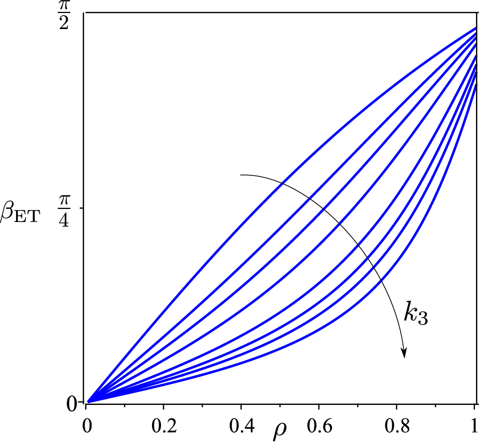
For reference, the values measured in Eun et al. 2019 correspond to e .
By use of both (29) and (33) in (25), we express in the form,
| (37) |
which by (32) can be written explicitly in terms of the reduced elastic constants only,
| (38) |
an expression that, for , can be shown to be negative in both instances, as the following inequalities hold true,
| (39) | ||||
| (40) |
, as given by (38) as a function of , is continuous along with its derivatives at .1111 11 Apart from a different scaling of the constant , the formula in (38) for coincides with equation (5) of Davidson et al. 2015a. Moreover, the same formula is also valid for the energy of the mirror image of . Thus, whenever the ET distortion is permitted, that is, for , it possesses less elastic free energy than the uniform alignment , and so it becomes eligible for the ground state of CLCs, at least within the cylindrical confinement investigated experimentally.
The price to pay to model mathematically the experimental observations with the ET distortion is to renounce one of Ericksen’s inequalities, thus accepting that Frank’s functional in (10) may be unbounded below, jeopardizing in general its coercivity. This has no noxious consequences whenever the degenerate boundary condition (15) is prescribed, as the integral in (16) is bounded below and the remaining terms in (1) are well-behaved, provided that the constants , , and are all positive. Instances are known in the literature where appropriate boundary conditions salvage a functional that in other, more general circumstances would fail to attain its minimum (see, for example, Day and Zarnescu 2019). Here a similar situation arises with the complicity of cylindrical symmetry. Fearing, however, a potentially latent pathology emerging from the lack of boundedness in the general setting, we find it especially appropriate to study the local stability of the ET distortion, albeit against perturbations that do not break cylindrical symmetry.
To this end in the following section we shall derive a general formula for the second variation of . Before that, we pause to illuminate further the ET field in terms of the distortion characteristics. By use of (30) in (19), (22), and (23), we see that (for the positive branch)
| (41a) | ||||
| (41b) | ||||
| (41c) | ||||
where as in (36) (with ), whereas for (the negative branch), changes its sign, as do , , and , while remains unchanged. Although the characteristics in (41) are all different from zero, in the limit as they yield
| (42) |
suggesting that each ET distortion has a single non-vanishing characteristic only along the cylinder’s axis. Being such a single distortion mode unable to fill space, it can be accommodated within the cylinder only by igniting all other modes. We may stress the non-uniformity of ET distortions by saying that they represent a pseudo ground state of CLCs, one that is bound to change from place to place in space. Alternatively, we may interpret their lack of uniformity as a result of elastic frustration induced by a cylindrical confinement, whose geometric measure transpires in (42) through the radius . In the following, we shall regard both ways of saying as semantic variants of the same physical notion.
III Second Variation
To compute the second variation of Frank’s elastic free-energy functional, we devise here a variant to the classical method: we represent a generic perturbation of a given director field via a path on the unit sphere parameterized in and going through the point . The mapping defines for each a trajectory in , which for satisfies . Thus, as the virtual time spans , the vector fields on are instantaneous realizations of diverse perturbations of . The constraint of unimodularity for must be valid for all , and so,
| (43) |
where a superimposed dot denotes differentiation with respect to . We define the field
| (44) |
which by (43) is orthogonal to ,
| (45) |
By further differentiating both sides of (43) with respect to , we arrive at
| (46) |
The field represents a second-order perturbation for . It follows from (46) and (44) that
| (47) |
where , precisely like , is an arbitrary vector field orthogonal to , and . We say that and are the first- and second-order outer variations of .
The first variation of at the field is a linear functional of defined as
| (48) |
An equilibrium director field makes vanish for all satisfying (45). With the aid of (44) and (100) we obtain that
| (49) |
with sufficiently regular.1212 12 The reader is deferred to Appendix B for a number of ancillary results used here.
Similarly, the second variation of at the field is the functional defined by
| (50) |
which is linear in and quadratic in . By use of (47) and (B), we give (50) the following form
| (51) |
which reduces to only its quadratic component in whenever is an equilibrium field. In this latter case, with a slight abuse of notation, we shall simply set .
III.1 Simple Applications
To put to the test the formula for the second variation of in (III), here we compute it for two special equilibrium fields.1313 13 Which are actually universal equilibrium fields, as they solve the equilibrium equations for any frame-indifferent elastic free-energy density , as shown in Ericksen 1967.
III.1.1 Uniform Field
We begin with a director field uniformly constant in space and see how its stability is related to Ericksen’s inequalities (7). With no loss of generality, for a given Cartesian frame , we apply (III) to the director field ,
| (52) |
where . It follows from this latter identity that
| (53) |
with and arbitrary vector fields. Letting and be the components of and in the frame , we easily compute
| (54a) | ||||
| (54b) | ||||
| (54c) | ||||
| (54d) | ||||
which give (52) the following form,
| (55) |
For a general domain with no boundary conditions for , the integrand on the right-hand side of (55) is the sum of three independent quadratic forms, so that is positive whenever all these forms are not negative, which is precisely when Ericksen’s inequalities (7) are satisfied.
III.1.2 Radial Hedgehog
The radial hedgehog is the director field that in the frame of spherical coordinates is represented as . Standard computations give , , and , so that (III) reduces to
| (56) |
For a sphere with center in the origin of the frame and under the strong anchoring condition , this formula coincides with equation (2.3) of Kinderlehrer and Ou 1992, where the second variation (56) was proven to be positive in the class of perturbations with compact support and satisfying , whenever the following inequality is satisfied,
| (57) |
IV Local Stability
In this section, we study the local stability of the ET field , delivered by (17) when as in (36). We shall focus our attention on this chiral variant of the ET field, as that with opposite chirality, represented by , has by symmetry the same energy and the same stability character.
In the scaled radial coordinate introduced in (24), the perturbation field , subject to , is represented in the frame of cylindrical coordinates as
| (58) |
where and are absolutely continuous functions on . The validity of the degenerate planar anchoring condition (15) for the perturbed director field requires that
| (59) |
while remains completely arbitrary. Moreover, for the regularity of along the cylinder’s axis (and the integrability of the perturbed energy), we also request that
| (60) |
Making use in (III) of the identities (103) recorded in Appendix B, we arrive at the following dimensionless form of the second variation in the class of perturbation fields described by (58),
| (61) |
where
| (62) |
while and are as in (26), and as in (36). Integrations by parts have been performed in (IV) by employing both (59) and (60).
In (IV) the scalar perturbations and are decoupled and can be regarded as the sum of two independent functionals. When and , we say that is an azimuthal perturbation. On the contrary, when and , we say that is a radial perturbation. We shall consider these perturbations separately below; the local stability of the field requires that be positive for both types of perturbation.
Our study will be limited to the case , which according to the experimental measurements of Zhou et al. 2012 and Zhou et al. 2014 is the only relevant to chromonics, the materials of interest to us in this work.
IV.1 Azimuthal Perturbations
To compute , we take advantage of the fact that is a monotonically increasing function of , ranging in the interval , with as in (32), as ranges in . This allows us to express as a function of , and ultimately as a function, , of the variable
| (63) |
which ranges in , as is defined by
| (64) |
This cascade of changes of variables is characterized by the following relations involving their differentials,
| (65) |
Their use gives the following, more compact form,
| (66) |
where a prime now denotes differentiation with respect to , we have set
| (67a) | ||||
| (67b) | ||||
| (67c) | ||||
and belongs to the admissible class
| (68) |
The elastic constants enter (66) through the pair of dimensionless parameters . It follows from (64) that ranges in for all and . Conversely, is expressed in terms of by
| (69) |
so that the correspondence between the half-space and the strip is one-to-one as the Jacobian determinant of the transformation is positive,
| (70) |
Here we show that for all the functional in (66) is positive definite in the class . Our desired conclusion will be reached in two steps. First, we see that the functions
| (71) |
obey all three conditions of Lemma 1 in Appendix B for and as in (67b). Thus, it follows from (104) that
| (72) |
Second, from the identity
| (73) |
we readily obtain that
| (74) |
Making use of (72) in (74) and integrating by parts, we finally arrive at
| (75) |
We are now in a position to conclude our proof, as combining (75) with (66) we estimate
| (76) |
and so, for to be positive on it suffices that the following inequalities are valid
| (77) |
which by (67) reduce to
| (78) |
and are easily seen to be valid for all and .
IV.2 Radial Perturbations
Now, we ignite the radial modes in the second variation in (IV), while silencing the azimuthal ones,
| (79) |
where and is subject to (60) and (59). Here, as suggested by the experimental evidence presented in Zhou et al. 2012; Zhou et al. 2014, we assume that for chromonics . This inequality, combined with the same changes of variables performed in Sect. IV.1, leads us to replace (66) with
| (80) |
where now
| (81) |
and is subject to the additional condition that .
Following the same lines of thought that in Sect. IV.1 established the lower bound (76), here we arrive at
| (82) |
and the following inequality suffices to render positive,
| (83) |
which is indeed satisfied for all and .
We thus conclude that the ET fields are locally stable, despite the violation of one Ericksen’s inequality.1414 14 A violation nonetheless necessary for these fields to be equilibrium solutions. Here we considered only the case ; for completeness, the local stability of the ET fields has also been established in the case by use of a spectral method Paparini 2022.
V Conclusions
In this article, we addressed the problem posed by the peculiar ground state exhibited by chromonic liquid crystals. These, unlikely ordinary nematic liquid crystals, when confined within capillary tubes with degenerate boundary conditions do not acquire the uniform alignment with the director oriented along the cylinder’s axis, but develop a spontaneous twist, equally likely to have opposite chiralities. A commonly accepted explanation for such a behaviour is that these materials have a twist elastic constant smaller than the saddle-splay constant of Frank’s elastic theory, a fact which has been confirmed by a number of experiments. The problem with this explanation is that assuming violates one of Ericksen’s inequalities, which guarantee that Frank’s elastic free energy is bounded below.
Very recently, such a violation has also been investigated in Long and Selinger 2022, which proposed that the pure (double) twist mode that would characterize the ground state of chromonics,1515 15 With only . being non-uniform and so unable to fill space Virga 2019, prompts the excitation of other elastic modes whose positive cost counterbalances the divergence to negative infinity of the total free energy. Here, concerned as we were by tackling a variational problem with indefinite energy, we gave a different, but complementary explanation. We showed that the boundary conditions prescribed on the capillary tubes are indeed responsible for taming the unboundedness of the energy and securing a solution to the variational problem in an admissible class of distortions with cylindrical symmetry.
The issue about the stability of such a solution then remained open, a question that was not idle to ask, given the wildness of the parent energy. To resolve this issue, we derived a general formula for the second variation of Frank’s elastic free-energy functional and applied it to the study of the (local) stability of the twisted ground state of chromonics. We concluded that this is stable.
The role played by boundary conditions in stabilizing the ground state of chromonics within the classical elastic theory of Frank poses at least two further questions. First, what is the most general class of anchoring conditions capable in rigid containers of preventing the energy from diverging to negative infinity? Second, and more subtly, would free boundaries, such as the ones arising in the equilibrium problem for a chromonic drop surrounded by its isotropic melt, keep the energy bounded below?
We have not tackled the first question. As for the second, preliminary explorations Paparini 2022 have shown that the violation of Ericksen’s inequalities for either the twist or splay constants may result in a paradoxical disintegration process, which poses a serious threat to the applicability of Frank’s elastic theory to chromonics. More details on such a threat will be given in a forthcoming paper Paparini and Virga 2022, where we shall also discuss the amendments to the classical elastic theory that may be needed for it to encompass chromonics safely.
Appendix A Dynamical Analogy
This Appendix is devoted to a dynamical interpretation of the free-energy functional in (25). In this interpretation, the first integral (29) will be regarded as a conservation law and the qualitative features of the equilibrium solution (36) will be derived from a phase plane analysis. Of course, nothing will be added to what we already know about the ET fields, but we shall perhaps appreciate better their stance amid other equilibrium configurations with unbounded energy.
We transform functional (25) into a dynamical action by introducing the artificial time
| (84) |
Thus, the axis of the cylinder at is approached as , while , the origin of time, corresponds to the surface of the lateral surface of . Correspondingly, the angle becomes a function of ,
| (85) |
and in (25) acquires the form of an infinite horizon action Agrachev, A. A. and Chittaro, F. C. 2009,
| (86) |
where, as customary, a superimposed dot denotes differentiation with respect to and
| (87) |
| (88) |
The associated Lagrangian is the classical sum of a kinetic energy and a potential,
| (89) |
in the single Lagrangian variable . It is perhaps less typical of a classical dynamical system the initial-value potential . The orbits of the system are all solutions to the equation of motion
| (90) |
which here reads simply as
| (91) |
This equation is subject to both initial and asymptotic conditions which stem from requiring stationarity of the action at the beginning and at the end of time,1616 16 Alternatively, we may say that equations (92) prescribe the sources of momentum at both ends of the time horizon.
| (92a) | ||||
| (92b) | ||||
While the latter requires that
| (93) |
the former identifies a locus in the phase plane for all admissible initial conditions,
| (94) |
A conservation law follows readily from (91),
| (95) |
where is an arbitrary constant. Since , it readily follows from (95) that the admissible values of fall in the range . The phase portrait of (95) in the plane is illustrated in Fig. 3 for .

Orbits are selected by the values of . For , the corresponding orbits collapse in the points . As increases, orbits are inflated and stay closed until (see green trajectories in Fig. 3). This latter value corresponds to orbits that converge to the origin and to the points (blue trajectories). The collectively act as a separatrix in phase plane, bounding the domain of closed orbits. For , orbits become unbounded (gray trajectories).
This qualitative analysis, based on the conservation law (95), embraces all possible orbits. We are especially interested in those that start from the admissible locus (94) in phase space and obey the asymptotic condition (93). The former is represented by the red curve in Fig. 3, while the latter requires the orbit to approach the -axis as . Now, if , the green trajectories are periodic orbits that keep crossing infinitely many times the -axis, whereas if the gray trajectories are open orbits that never cross the -axis. Only for , that is, along the separatrix, can an orbit approach the -axis starting from an admissible initial condition.
As shown in Fig. 3, there is a critical value of corresponding to orbits tangent to the curve of admissible initial conditions,
| (96) |
For , the open orbits of the system are inadmissible. For and , the orbits obey (92a), but violate (92b); their total action in (86), which by (95) can be expressed as
| (97) |
is easily seen to be unbounded.
Contrariwise, for , the total action is finite and can be shown to equal the elastic free energy computed in (37). The rate at which time diverges as the origin in phase space is approached (on a the separatrix) can be estimated as
| (98) |
see Paparini 2022 for more quantitative details.
We have learned in Sect. II that the equilibrium solution in (36) only exists for . This also arises from the dynamical analogy studied here and is revealed by a geometric feature of the phase portrait. As can be shown by an asymptotic expansion of both (94) and (95) near the origin, for , the curve of admissible initial conditions lies inside the separatrix, and so there is no admissible orbit with finite total action. Figure 4 illustrates graphically the situation; in particular, for and , the curve of admissible initial conditions is (internally) tangent to the separatrix.


Appendix B Useful Identities and Inequalities
We collect in this Appendix a number of identities and inequalities that are used in the main text.
For the mapping introduced in Sect. III, we compute the following derivatives with respect to the parameter ,
| (99) |
and
| (100) |
By use of these in (1), we readily obtain that
| (101) |
and
| (102) |
For a director field as in (17), whose gradient has been computed in (18), and for the perturbation field described in (58), the following computational ingredients were needed in the main text to arrive from the general formula for the second variation of Frank’s elastic free energy in (III) at the special form needed when the unperturbed field in ,
| (103a) | ||||
| (103b) | ||||
| (103c) | ||||
| (103d) | ||||
| (103e) | ||||
| (103f) | ||||
| (103g) | ||||
| (103h) | ||||
| (103i) | ||||
| (103j) | ||||
| (103k) | ||||
| (103l) | ||||
| (103m) | ||||
| (103n) | ||||
| (103o) | ||||
where a prime denotes differentiation with respect to .
A family of inequalities has played a central role in Sect. IV. They stem from the adaptation to our setting of a Lemma proved in Li and Yeh 1995 (see Lemma 2.1).
Lemma 1.
Let be an interval in and let . If there are two functionals, and , satisfying the following conditions
- 1.
is in the range of the function ,
- 2.
is integrable for ,
- 3.
is absolutely continuous for ,
then
| (104) |
where and .
References
- Dickinson et al. (2009) A. J. Dickinson, N. D. LaRacuente, C. B. McKitterick, and P. J. Collings, Aggregate structure and free energy changes in chromonic liquid crystals, Mol. Cryst. Liq. Cryst. 509, 751 (2009).
- Tam-Chang and Huang (2008) S.-W. Tam-Chang and L. Huang, Chromonic liquid crystals: properties and applications as functional materials, Chem. Commun. 44, 1957 (2008).
- Mariani et al. (2009) P. Mariani, F. Spinozzi, F. Federiconi, H. Amenitsch, L. Spindler, and I. Drevensek-Olenik, Small angle X-ray scattering analysis of deoxyguanosine 5’-monophosphate self-assembing in solution: Nucleation and growth of G-quadruplexes, J. Phys. Chem. B 113, 7934 (2009).
- Zanchetta et al. (2008) G. Zanchetta, M. Nakata, M. Buscaglia, T. Bellini, and N. A. Clark, Phase separation and liquid crystallization of complementary sequences in mixtures of nanodna oligomers, Proc. Natl. Acad. Sci. USA 105, 1111 (2008).
- Nakata et al. (2007) M. Nakata, G. Zanchetta, B. D. Chapman, C. D. Jones, J. O. Cross, R. Pindak, T. Bellini, and N. A. Clark, End-to-end stacking and liquid crystal condensation of 6- to 20-base pair DNA duplexes, Science 318, 1276 (2007).
- Fraccia and Jia (2020) T. P. Fraccia and T. Z. Jia, Liquid crystal coacervates composed of short double-stranded dna and cationic peptides, ACS Nano 14, 15071 (2020).
- Lydon (1998a) J. Lydon, Chromonic liquid crystal phases, Curr. Opin. Colloid Interface Sci. 3, 458 (1998a).
- Lydon (1998b) J. Lydon, Chromonics, in Handbook of Liquid Crystals: Low Molecular Weight Liquid Crystals II (John Wiley & Sons, Weinheim, Germany, 1998) Chap. XVIII, pp. 981–1007.
- Lydon (2010) J. Lydon, Chromonic review, J. Mater. Chem. 20, 10071 (2010).
- Lydon (2011) J. Lydon, Chromonic liquid crystalline phases, Liq. Cryst. 38, 1663 (2011).
- Dierking and Martins Figueiredo Neto (2020) I. Dierking and A. Martins Figueiredo Neto, Novel trends in lyotropic liquid crystals, Crystals 10, 604 (2020).
- Nayani et al. (2015) K. Nayani, R. Chang, J. Fu, P. W. Ellis, A. Fernandez-Nieves, J. O. Park, and M. Srinivasarao, Spontaneous emergence of chirality in achiral lyotropic chromonic liquid crystals confined to cylinders, Nat. Commun. 6, 8067 (2015).
- Onsager (1949) L. Onsager, The effects of shape on the interaction of colloidal particles, Ann. N. Y. Acad. Sci. 51, 627 (1949).
- Xiao et al. (2014) W. Xiao, C. Hu, D. J. Carter, S. Nichols, M. D. Ward, P. Raiteri, A. L. Rohl, and B. Kahr, Structural correspondence of solution, liquid crystal, and crystalline phases of the chromonic mesogen sunset yellow, Crystal Growth Des. 14, 4166 (2014).
- Park et al. (2008) H.-S. Park, S.-W. Kang, L. Tortora, Y. Nastishin, D. Finotello, S. Kumar, and O. D. Lavrentovich, Self-assembly of lyotropic chromonic liquid crystal sunset yellow and effects of ionic additives, J. Phys. Chem. B 112, 16307 (2008).
- Kleman and Lavrentovich (2003) M. Kleman and O. D. Lavrentovich, Soft Matter Physics: An Introduction, Partially Ordered Systems (Springer-Verlag, New York, 2003).
- Pišljar et al. (2022) J. Pišljar, S. Ghosh, S. Turlapati, N. V. S. Rao, M. Škarabot, A. Mertelj, A. Petelin, A. Nych, M. Marinčič, A. Pusovnik, M. Ravnik, and I. Muševič, Blue phase III: Topological fluid of skyrmions, Phys. Rev. X 12, 011003 (2022).
- Meiboom et al. (1981a) S. Meiboom, J. P. Sethna, P. W. Anderson, and W. F. Brinkman, Theory of the blue phase of cholesteric liquid crystals, Phys. Rev. Lett. 46, 1216 (1981a), see also Erratum Meiboom et al. 1981b.
- Meiboom et al. (1983) S. Meiboom, M. Sammon, and W. F. Brinkman, Lattice of disclinations: The structure of the blue phases of cholesteric liquid crystals, Phys. Rev. A 27, 438 (1983).
- Saupe (1969) A. Saupe, On molecular structure and physical properties of thermotropic liquid crystals, Mol. Cryst. Liq. Cryst. 7, 59 (1969).
- Davidson et al. (2015a) Z. S. Davidson, L. Kang, J. Jeong, T. Still, P. J. Collings, T. C. Lubensky, and A. G. Yodh, Chiral structures and defects of lyotropic chromonic liquid crystals induced by saddle-splay elasticity, Phys. Rev. E 91, 050501(R) (2015a), see also Erratum Davidson et al. 2015b.
- Burylov (1997) S. Burylov, Equilibrium configuration of a nematic liquid crystal confined to a cylindrical cavity, J. Exp. Theor. Phys 85, 873 (1997).
- Frank (1958) F. C. Frank, On the theory of liquid crystals, Discuss. Faraday Soc. 25, 19 (1958).
- Zocher (1933) H. Zocher, The effect of a magnetic field on the nematic state, Trans. Faraday Soc. 29, 945 (1933).
- Oseen (1933) C. W. Oseen, The theory of liquid crystals, Trans. Faraday Soc. 29, 883 (1933).
- Virga (1994) E. G. Virga, Variational Theories for Liquid Crystals, Applied Mathematics and Mathematical Computation, Vol. 8 (Chapman & Hall, London, 1994).
- Selinger (2018) J. V. Selinger, Interpretation of saddle-splay and the Oseen-Frank free energy in liquid crystals, Liq. Cryst. Rev. 6, 129 (2018).
- Machon and Alexander (2016) T. Machon and G. P. Alexander, Umbilic lines in orientational order, Phys. Rev. X 6, 011033 (2016).
- Selinger (2022) J. V. Selinger, Director deformations, geometric frustration, and modulated phases in liquid crystals, Ann. Rev. Condens. Matter Phys. 13 (2022), First posted online on October 12, 2021. Volume publication date, March 2022.
- Pedrini and Virga (2020) A. Pedrini and E. G. Virga, Liquid crystal distortions revealed by an octupolar tensor, Phys. Rev. E 101, 012703 (2020).
- Ericksen (1966) J. L. Ericksen, Inequalities in liquid crystal theory, Phys. Fluids 9, 1205 (1966).
- Virga (2019) E. G. Virga, Uniform distortions and generalized elasticity of liquid crystals, Phys. Rev. E 100, 052701 (2019).
- Meyer (1976) R. B. Meyer, Structural problems in liquid crystal physics, in Molecular Fluids, Les Houches Summer School in Theoretical Physics, Vol. XXV-1973, edited by R. Balian and G. Weill (Gordon and Breach, New York, 1976) pp. 273–373.
- Cestari et al. (2011) M. Cestari, S. Diez-Berart, D. A. Dunmur, A. Ferrarini, M. R. de la Fuente, D. J. B. Jackson, D. O. Lopez, G. R. Luckhurst, M. A. Perez-Jubindo, R. M. Richardson, J. Salud, B. A. Timimi, and H. Zimmermann, Phase behavior and properties of the liquid-crystal dimer 1′′,7′′-bis(4-cyanobiphenyl-4′-yl) heptane: A twist-bend nematic liquid crystal, Phys. Rev. E 84, 031704 (2011).
- Ericksen (1962) J. L. Ericksen, Nilpotent energies in liquid crystal theory, Arch. Rational Mech. Anal. 10, 189 (1962).
- Koning et al. (2014) V. Koning, B. C. van Zuiden, R. D. Kamien, and V. Vitelli, Saddle-splay screening and chiral symmetry breaking in toroidal nematics, Soft Matter 10, 4192 (2014).
- Eun et al. (2019) J. Eun, S.-J. Kim, and J. Jeong, Effects of chiral dopants on double-twist configurations of lyotropic chromonic liquid crystals in a cylindrical cavity, Phys. Rev. E 100, 012702 (2019).
- Day and Zarnescu (2019) S. Day and A. D. Zarnescu, Sphere-valued harmonic maps with surface energy and the k13 problem, Adv. Calc. Var. 12, 363 (2019).
- Ericksen (1967) J. L. Ericksen, General solutions in the hydrostatic theory of liquid crystals, Trans. Soc. Rheol. 11, 5 (1967).
- Kinderlehrer and Ou (1992) D. Kinderlehrer and B. Ou, Second variation of liquid crystal energy at , Proc. R. Soc. Lond. A 437, 475 (1992).
- Zhou et al. (2012) S. Zhou, Y. A. Nastishin, M. M. Omelchenko, L. Tortora, V. G. Nazarenko, O. P. Boiko, T. Ostapenko, T. Hu, C. C. Almasan, S. N. Sprunt, J. T. Gleeson, and O. D. Lavrentovich, Elasticity of lyotropic chromonic liquid crystals probed by director reorientation in a magnetic field, Phys. Rev. Lett. 109, 037801 (2012).
- Zhou et al. (2014) S. Zhou, K. Neupane, Y. A. Nastishin, A. R. Baldwin, S. V. Shiyanovskii, O. D. Lavrentovich, and S. Sprunt, Elasticity, viscosity, and orientational fluctuations of a lyotropic chromonic nematic liquid crystal disodium cromoglycate, Soft Matter 10, 6571 (2014).
- Paparini (2022) S. Paparini, Mathematical Models for Chromonic Liquid Crystals, Ph.D. thesis, Joint PhD Program in Mathematics, Pavia - Milano Bicocca - INdAM, Milan (2022).
- Long and Selinger (2022) C. Long and J. V. Selinger, Violation of Ericksen inequalities in lyotropic chromonic liquid crystals (2022), arXiv:2202.00184 [cond-mat.soft].
- Paparini and Virga (2022) S. Paparini and E. G. Virga, Paradoxes for chromonic liquid crystals, (2022), unpublished.
- Agrachev, A. A. and Chittaro, F. C. (2009) Agrachev, A. A. and Chittaro, F. C., Smooth optimal synthesis for infinite horizon variational problems, ESAIM: COCV 15, 173 (2009).
- Li and Yeh (1995) H. J. Li and C. C. Yeh, Inequalities for a function involving its integral and derivative, Proc. R. Soc. Edinb. A 125, 133 (1995).
- Meiboom et al. (1981b) S. Meiboom, J. P. Sethna, P. W. Anderson, and W. F. Brinkman, Theory of the blue phase of cholesteric liquid crystals., Phys. Rev. Lett. 46, 1656 (1981b).
- Davidson et al. (2015b) Z. S. Davidson, L. Kang, J. Jeong, T. Still, P. J. Collings, T. C. Lubensky, and A. G. Yodh, Erratum: Chiral structures and defects of lyotropic chromonic liquid crystals induced by saddle-splay elasticity [Phys. Rev. E 91, 050501(R) (2015)], Phys. Rev. E 92, 019905 (2015b).