A Laser-Atom Interaction Simulator derived from Quantum ElectrodynamicsPreprint: APS/123-QED

Laser-excitation of atoms is an essential physical process used in many experiments including spectroscopy Neugart et al. 2017; Studer et al. 2019, trapping of atoms Raab et al. 1987; Harvey and Murray 2008; Cortiñas et al. 2020; Urvoy et al. 2019, collision physics Hertel and Stoll 1978; Farrell et al. 1988; MacGillivray and Standage 1988; Murray et al. 1989; Murray et al. 1990; Farrell et al. 1991; Murray et al. 1991a; Murray et al. 1992; Murray et al. 1991b; Masters et al. 1996; Murray and Cvejanovic 2003; Hussey et al. 2007; Murray et al. 2008; Hussey et al. 2008; Nixon and Murray 2011; Nixon and Murray 2014 and atomic interferometry Rudolph et al. 2020. To design experiments such as these, modelling of the dynamics of the laser-atom interaction with time is often required. The semi-classical approach to solving the equation of motions of these systems has been used extensively, where the atom is quantized and the field is treated classically McClelland and Kelley 1985; Robertson et al. 2021; Stenholm 1986; Milošević 2017. In these models the relaxation terms are added phenomenologically. By contrast, models that treat both the atom and field quantum mechanically can describe the relaxation terms more rigorously, particularly when the system is complex with many substates involved in the interaction Farrell et al. 1988. Deriving the equations of motion (often called the optical Bloch equations) by hand and solving the laser-atom interaction is time-intensive, complex, and is prone to mistakes. As an example, for transitions with hyperfine structure such as excitation of the Cs 6${}^{2}S_{1/2}$ state to the 6${}^{2}P_{3/2}$ state, a total of 48 individual substates are involved in the interaction. There are hence 2304 coupled differential equations that must be generated and solved simultaneously to fully characterise the dynamics of the system. A computational method of systematically generating and solving these equations is hence advantageous, so that the time evolution of the populations, optical coherences and the atomic coherences can be obtained.

This paper presents an open-source python package that solves this problem: a laser-atom interaction simulator derived from quantum electrodynamics (LASED). LASED allows a user to automatically set up a laser-atom system and generate all the equations of motion for that system, which can be printed out in LaTeX. The package then solves the dynamics of the system over a given time, outputting the evolution of all lower and upper state populations, their atomic coherences and the optical coherence terms that couple the states together. LASED can also model the system using laser beams that have different polarizations. It can model a rotation of the frame of reference of the system both prior to the interaction, as well as after the laser interaction has occurred. This rotation technique can simplify the calculation, thereby reducing the time required for generating an output. LASED can further include integration over the Gaussian profile of the laser beam (assuming a TEM₀₀ beam) and also allows integration over the Doppler profile of an atomic beam, should this be required for the experiment that is being modelled. The angular ‘shape’ of the electron charge cloud for both excited and lower atomic states can also be modelled and plotted as the system evolves over time.

Other laser-atom interaction simulators exist that are used to describe different processes. The simulator described in Eckel et al. 2022 has been developed to model atoms that are laser-cooled in a magneto-optical trap, and includes the effect of the trapping magnetic field as well as the laser field. LASED has been developed in a similar way, however it can also describe different experiments such as scattering experiments that combine laser interactions with electron collisions and that use an atomic beam Hertel and Stoll 1978; Farrell et al. 1988; MacGillivray and Standage 1988; Murray et al. 1989; Murray et al. 1990; Farrell et al. 1991; Murray et al. 1991a; Murray et al. 1992; Murray et al. 1991b; Masters et al. 1996; Murray and Cvejanovic 2003; Hussey et al. 2007; Murray et al. 2008; Hussey et al. 2008; Nixon and Murray 2011; Nixon and Murray 2014. LASED is designed to be easy-to-use and has comprehensive online documentation to aid users in creating the required laser-atom system they wish to model. This documentation also demonstrates how to run the simulations by solving examples of the differential equations automatically generated by LASED Patel 2021a. Details on how to install LASED can be found in this documentation and in appendix C.

In this paper the derivation of the general equations of motion which are adopted in LASED are briefly presented in section II. In section III the computational method for generating the coupled differential equations to solve the time evolution of the laser-atom system is discussed. This section also shows how averaging over the Gaussian and Doppler profiles is approximated, and it details how the reference frame is rotated. The method used to model a general polarization state of the laser is also described.

Section IV demonstrates the outcome from the model for three selected targets. In the first example excitation of calcium from the ground 4$S$ state to the 4$P$ state is discussed, since this is one of the simplest systems that can be solved. These results are presented for both linear and elliptic excitation, and includes integration over both Doppler and Gaussian profiles. An example of the technique of rotating the frame of reference is then discussed, with the calcium target again being used. In the second example, laser excitation of helium initially excited by electron impact to a $D$-state is presented. This is a considerably more complex problem to solve, since the lower state is then in a coherent superposition of substates due to the collision. Both the populations and atomic coherences are hence non-zero prior to laser excitation and these must be included as initial conditions. Finally, a discussion of laser excitation of the Cs atom from the ground state via the $D_{2}$ transition is presented for circular excitation, as would be used in a Magneto Optical Trap (MOT).

The general equations of motion using the QED approach for continuous wave laser irradiation of atoms have been detailed in Farrell et al. 1988; Farrell et al. 1991; MacGillivray and Standage 1988; Murray et al. 2008, and so only a brief overview is presented here. The equations are derived using the Heisenberg formulation, where the operators are chosen to evolve in time. The Hamiltonian of the laser-atom system is hence given by

$$H=H_{\textrm{Atom}}+H_{\textrm{Field}}+H_{\textrm{Int}}$$

(1)

where $H_{\textrm{Atom}}$ describes the atom evolving freely over time, so that

$$H_{\textrm{Atom}}=\sum_{i}\hbar\omega_{i}|{i}\rangle\langle{i}|$$

(2)

where $\hbar\omega_{i}$ is the energy of the $i$’th level. The Hamiltonian for the field is represented quantum mechanically by

$$H_{\textrm{Field}}=\sum_{q}\hbar\omega_{q}a_{q}^{\dagger}a_{q}$$

(3)

where $a_{q}^{\dagger}$,$a_{q}$ are the creation and annihilation operators for the mode $q$ of the field, with $q$ representing both the wave vector and its polarization. The interaction Hamiltonian Loudon 2000 is expressed in normal ordering Ackerhalt and Eberly 1974 as

$$H_{\textrm{Int}}=\hbar\sum_{e^{\prime}g^{\prime}q^{\prime}}g^{q^{\prime}}_{e^{\prime}g^{\prime}}\hat{\sigma}_{e^{\prime}g^{\prime}}a_{q^{\prime}}e^{ik_{q^{\prime}}z}+g^{q^{\prime}*}_{e^{\prime}g^{\prime}}a^{\dagger}_{q^{\prime}}e^{-ik_{q^{\prime}}z}\hat{\sigma}_{g^{\prime}e^{\prime}}$$

(4)

where

$$g^{q^{\prime}}_{e^{\prime}g^{\prime}}=i\sqrt{\frac{\omega_{q^{\prime}}}{2\epsilon_{0}\hbar{V}}}\hat{\textbf{e}}_{q^{\prime}}.\textbf{D}_{e^{\prime}g^{\prime}}$$

(5)

is a coupling coefficient between the mode of the laser field and the lower atomic state $|{g^{\prime}}\rangle$ and upper state $|{e^{\prime}}\rangle$. $V$ is the mode volume, $\textbf{D}_{e^{\prime}g^{\prime}}$ is the dipole moment, and $\hat{\textbf{e}}_{q^{\prime}}$ is the polarization unit vector. The atomic operators are defined by the atomic states so that

$$\hat{\sigma}_{eg}=|{e}\rangle\langle{g}|.$$

(6)

where $|{g}\rangle$ represents the manifold of all lower states of the system and $|{e}\rangle$ represents the manifold of upper states that are coupled to $|{g}\rangle$ by the laser. The atomic operators evolve over time using the Liouville equation Kubo 1963

	$\displaystyle\frac{d\hat{\sigma}_{eg}}{dt}$	$\displaystyle=-\frac{i}{\hbar}[\hat{\sigma}_{eg},H]$
		$\displaystyle=-\frac{i}{\hbar}[\hat{\sigma}_{eg},H_{Atom}]-\frac{i}{\hbar}[\hat{\sigma}_{eg},H_{Int}].$		(7)

$H_{\textrm{Field}}$ does not contribute here as it commutes with the atomic operator. The first term in equation II can be simplified using the ortho-normality relations $\langle{e}|e\rangle=\langle{g}|g\rangle=1$ and $\langle{e}|g\rangle=\langle{g}|e\rangle=0$ so that

$$-\frac{i}{\hbar}[\hat{\sigma}_{eg},H_{\textrm{Atom}}]=-i(\omega_{g}-\omega_{e})|{e}\rangle\langle{g}|$$

(8)

The second term in equation II can be expanded using equation 4 so that

	$\displaystyle-\frac{i}{\hbar}[\hat{\sigma}_{eg},H_{\textrm{Int}}]=$	$\displaystyle-i\sum_{e^{\prime}q^{\prime}}g^{q^{\prime}*}_{e^{\prime}g}a_{q^{\prime}}(t)^{\dagger}e^{-ik_{q^{\prime}}z}\hat{\sigma_{ee^{\prime}}}$
	$\displaystyle+$	$\displaystyle i\sum_{g^{\prime}q^{\prime}}g^{q^{\prime}*}_{eg^{\prime}}a_{q}^{\dagger}e^{-ik_{q}z}\hat{\sigma}_{gg^{\prime}}$		(9)

As the time evolution of the annihilation and creation operators depends on the field coupling to the atomic states, an explicit function in time is required. For $a_{q}^{\dagger}$ this is given by

	$\displaystyle a^{\dagger}_{q^{\prime}}(t)=$	$\displaystyle a^{\dagger}_{q^{\prime}}(0)e^{i\omega_{q^{\prime}}t}$		(10)
		$\displaystyle+i\sum_{e^{\prime\prime}g^{\prime\prime}}g^{q^{\prime}}_{e^{\prime\prime}g^{\prime\prime}}e^{ik_{q^{\prime}}z}\int^{t}_{0}\hat{\sigma}_{e^{\prime\prime}g^{\prime\prime}}(t^{\prime})e^{i\omega_{q^{\prime}}(t-t^{\prime})}dt$

with $a_{q}$ given by the complex conjugate of this equation. In equation 10 the atomic operator can be removed from the integral using the Harmonic approximation Whitley and Stroud Jr 1976. When combined with equation II, this then yields

	$\displaystyle-\frac{i}{\hbar}[\hat{\sigma}_{eg},H_{\textrm{Int}}]=$	$\displaystyle-i\sum_{q^{\prime}e^{\prime}}g^{q^{\prime}*}_{e^{\prime}g}a_{q^{\prime}}^{\dagger}(0)e^{i({\omega_{q^{\prime}}t-k_{q^{\prime}}}z)}\hat{\sigma}_{ee^{\prime}}$
		$\displaystyle+\sum_{q^{\prime}e^{\prime}e^{\prime\prime}g^{\prime\prime}}\Big(g^{q^{\prime}*}_{e^{\prime}g}g^{q^{\prime}}_{e^{\prime\prime}g^{\prime\prime}}\hat{\sigma}_{e^{\prime\prime}g^{\prime\prime}}$
		$\displaystyle\times\int^{t}_{0}e^{i(\omega_{q^{\prime}}-\omega_{e^{\prime\prime}}+\omega_{g^{\prime\prime}}(t-t^{\prime}))}dt^{\prime}\Big)\hat{\sigma}_{ee^{\prime}}$
		$\displaystyle+i\sum_{q^{\prime}g^{\prime}}g^{q^{\prime}}_{eg^{\prime}}a^{\dagger}_{q^{\prime}}(0)e^{i\omega_{q^{\prime}}t-k_{q^{\prime}z}}\hat{\sigma}_{g^{\prime}g}$
		$\displaystyle-\sum_{q^{\prime}g^{\prime}e^{\prime\prime}g^{\prime\prime}}\Big(g^{q^{\prime}*}_{eg^{\prime}}g^{q^{\prime}}_{e^{\prime\prime}g^{\prime\prime}}{\hat{\sigma}_{e^{\prime\prime}g^{\prime\prime}}}$
		$\displaystyle\times\int^{t}_{0}e^{i(\omega_{q^{\prime}}-\omega_{e^{\prime\prime}}+\omega_{g^{\prime\prime}}(t-t^{\prime}))}dt^{\prime}\Big)\hat{\sigma}_{g^{\prime}g}.$		(11)

When the laser frequency $\omega_{q^{\prime}}$ is close to the transition frequency $\omega_{e^{\prime\prime}}-\omega_{g^{\prime\prime}}$ and for time periods much larger than the inverse of the oscillation frequency, the integrals in equation II can be approximated to $\delta$ functions Ackerhalt and Eberly 1974. The time evolution of the atomic operator can hence be written as

	$\displaystyle\frac{d\hat{\sigma}_{eg}}{dt}=$	$\displaystyle-i(\omega_{g}-\omega_{e}){\hat{\sigma}_{eg}}$
		$\displaystyle-i\sum_{q^{\prime}e^{\prime}}g^{q^{\prime}}_{e^{\prime}g}a^{\dagger}_{q^{\prime}}(0)e^{i(\omega_{q^{\prime}}t-k_{q^{\prime}}z)}\hat{\sigma}_{ee^{\prime}}$
		$\displaystyle+i\sum_{q^{\prime}g}g^{q^{\prime}*}_{eg^{\prime}}a^{\dagger}_{q^{\prime}}(0)e^{i(\omega_{q^{\prime}t-k_{q^{\prime}}z})}\hat{\sigma}_{g^{\prime}g}$
		$\displaystyle-\sum_{q^{\prime}g^{\prime}e^{\prime}}g^{q^{\prime}*}_{eg^{\prime}}g^{q^{\prime}}_{e^{\prime}g^{\prime}}\hat{\sigma}_{e^{\prime}g}\pi\delta(\omega_{q^{\prime}}-\omega_{e^{\prime}}+\omega_{g^{\prime}}).$		(12)

Equation II contains rapidly oscillating terms at the frequency of the driving radiation. In many experiments these cannot be measured, and so the Rotating Wave Approximation (RWA) Whitley and Stroud Jr 1976 is adopted. For a single mode continuous wave laser beam driving the transition, the RWA transforms the atomic operators into slowly varying operators $\hat{\chi}_{eg}$, by setting

		$\displaystyle\hat{\sigma}_{eg}=\hat{\chi}_{eg}e^{i(\omega_{L}t-k_{L}z)}$		(13)
		$\displaystyle\hat{\sigma_{gg^{\prime}}}=\hat{\chi}_{gg^{\prime}}$		(14)
		$\displaystyle\hat{\sigma_{ee^{\prime}}}=\hat{\chi}_{ee^{\prime}},$		(15)

where $\omega_{L}$ is the laser frequency and $k_{L}$ is the associated wave vector. Equation II is hence transformed to slowly varying operators using equation 13. Expectation values are then taken, so that

	$\displaystyle\langle\dot{\hat{\chi}}_{eg}\rangle=$	$\displaystyle-i(\omega_{L}-k_{L}\dot{z}-\omega_{eg})\langle\hat{\chi}_{eg}\rangle$
		$\displaystyle-i\sum_{Le^{\prime}}g^{L*}_{e^{\prime}g}\langle{a_{L}^{\dagger}(0)}\rangle\langle\hat{\chi}_{ee^{\prime}}\rangle$
		$\displaystyle+i\sum_{Lg^{\prime}}g^{L*}_{eg^{\prime}}\langle a_{L}^{\dagger}(0)\rangle\langle\hat{\chi}_{g^{\prime}g}\rangle$
		$\displaystyle-\sum_{qg^{\prime}e^{\prime}}g^{q*}_{eg^{\prime}}g^{q}_{e^{\prime}g^{\prime}}\langle\hat{\chi}_{e^{\prime}g}\rangle\pi\delta(\omega_{L}-\omega_{e^{\prime}}+\omega_{g^{\prime}}).$		(16)

The slowly varying operators are directly related to the density matrix elements $\rho_{eg}$ that are commonly used to describe the populations and coherences of an atomic system, since

$$\langle\hat{\chi}_{eg}\rangle=\langle{\psi}|e\rangle\langle{g}|\psi\rangle=(\langle{e}|\psi\rangle\langle{\psi}|g\rangle)^{*}=(\rho_{eg})^{*}=\rho_{ge}.$$

(17)

The half-Rabi frequency is input to equation II using the relation Farrell et al. 1988

$$\Omega^{L}_{eg}=g^{L*}_{eg}\langle\hat{a}_{L}^{\dagger}(0)\rangle.$$

(18)

This is set to be real by an appropriate choice of phase Farrell et al. 1988.

The time evolution of $\langle\dot{\hat{\chi}}_{gg^{\prime\prime}}\rangle$ and $\langle\dot{\hat{\chi}}_{ee^{\prime\prime}}\rangle$ can be derived in an identical way to that of $\langle\dot{\hat{\chi}}_{eg}\rangle$ in equation II. These can then be written in the density matrix formalism using equation 17. The general equations of motion for the populations, optical and atomic coherences as used in LASED are then given by:

	$\displaystyle\dot{\rho}_{gg^{\prime\prime}}=$	$\displaystyle-i\Delta_{gg^{\prime\prime}}\rho_{gg^{\prime\prime}}+i\sum_{Le}(\Omega^{L}_{eg^{\prime\prime}}\rho_{ge}-\Omega^{L}_{eg}\rho_{eg^{\prime\prime}})$
		$\displaystyle+\sum_{qe^{\prime}e^{\prime\prime}}g^{q}_{e^{\prime}g^{\prime\prime}}g^{q*}_{e^{\prime\prime}g}\pi\delta(\omega_{q}-\Delta_{e^{\prime\prime}g})\rho_{e^{\prime\prime}e^{\prime}}$
		$\displaystyle+\sum_{qe^{\prime}e^{\prime\prime}}g^{q}_{e^{\prime\prime}g^{\prime\prime}}g^{q*}_{e^{\prime}g}\pi\delta(\omega_{q}-\Delta_{e^{\prime\prime}g^{\prime\prime}})\rho_{e^{\prime}e^{\prime\prime}}$		(19)

	$\displaystyle\dot{\rho}_{ee^{\prime\prime}}=$	$\displaystyle-i\Delta_{ee^{\prime\prime}}\rho_{ee^{\prime\prime}}+i\sum_{Lg}(\Omega^{L}_{e^{\prime\prime}g}\rho_{eg}-\Omega^{L}_{eg}\rho_{ge^{\prime\prime}})$
		$\displaystyle-\sum_{qg^{\prime}e^{\prime}}g^{q}_{eg^{\prime}}g^{q*}_{e^{\prime}g^{\prime}}\pi\delta(\omega_{q}-\Delta_{e^{\prime}g^{\prime}})\rho_{e^{\prime}e^{\prime\prime}})$
		$\displaystyle-\sum_{qg^{\prime}e^{\prime}}g_{e^{\prime}g^{\prime}}^{q}g_{e^{\prime\prime}g^{\prime}}^{q*}\pi\delta(\omega_{q}-\Delta_{e^{\prime}g^{\prime}})\rho_{ee^{\prime}}$		(20)

	$\displaystyle\dot{\rho}_{ge}=$	$\displaystyle-i\Delta_{L,eg}\rho_{ge}-i\sum_{Le^{\prime}}\Omega_{e^{\prime}g}^{L}\rho_{e^{\prime}e}+i\sum_{Lg^{\prime}}\Omega_{eg^{\prime}}^{L}\rho_{gg^{\prime}}$
		$\displaystyle-\sum_{qg^{\prime}e^{\prime}}g_{e^{\prime}g^{\prime}}^{q}g_{eg^{\prime}}^{q*}\pi\delta(\omega_{q}-\Delta_{e^{\prime}g^{\prime}})\rho_{ge^{\prime}}$		(21)

with $\dot{\rho}_{eg}$ given by the complex conjugate of equation 21.

The population equations for the lower and upper states are derived by setting $g=g^{\prime}$ and $e=e^{\prime}$ respectively in equations 19 and 20. The atomic coherence equations (which describe the phase relationship between sub-states in each manifold) are formulated by setting $g\neq g^{\prime}$ and $e\neq e^{\prime}$ in these equations. The optical and non-optical terms between the lower and upper states manifolds are described by equation 21. This equation hence is used to derive both the optical coherence terms generated directly by the laser, as well as the atomic coherence terms generated between upper and lower states. The term

$$\Delta_{L,eg}=\omega_{L}-\frac{2\pi v_{z}}{\lambda_{L}}+\omega_{e}-\omega_{g}$$

(22)

is the detuning from resonance, where $v_{z}$ is the velocity component of the atoms in the direction of the laser beam (which gives rise to the Doppler shift). $\lambda_{L}$ is the wavelength of the laser mode $L$. The term $\Delta_{eg}=\omega_{e}-\omega_{g}$, whereas $\Delta_{gg^{\prime}}=\omega_{g}-\omega_{g^{\prime}}$ and $\Delta_{ee^{\prime}}=\omega_{e}-\omega_{e^{\prime}}$. The half-Rabi frequency can be calculated in rad/s using the expression

$$\Omega_{eg}^{q}=C_{eg}^{q}\Omega=C_{eg}^{q}\sqrt{\frac{3\lambda_{L}^{3}I_{L}}{8{\pi}hc\tau}}$$

(23)

where $\tau$ is the lifetime of the transition, $I_{L}$ is the laser intensity, and $C^{q}_{eg}$ is a coupling coefficient given by Farrell and MacGillivray 1995

	$\displaystyle C^{q}_{eg}=$	$\displaystyle(-1)^{\frac{q(1+q)}{2}+F^{\prime}+F+J^{\prime}+J+I^{\prime}+L^{\prime}+S^{\prime}-m_{F}^{\prime}+1}$
		$\displaystyle\times\sqrt{(2F^{\prime}+1)(2F+1)(2J^{\prime}+1)(2J+1)(2L^{\prime}+1)}$
		$\displaystyle\times\begin{pmatrix}F^{\prime}&1&F\\ -m_{F}^{\prime}&q&m_{F}\end{pmatrix}\begin{Bmatrix}J^{\prime}&F^{\prime}&I^{\prime}\\ F&J&1\end{Bmatrix}\begin{Bmatrix}L^{\prime}&J^{\prime}&S^{\prime}\\ J&L&1\end{Bmatrix}$		(24)

where $L,S,J,I$, and $F$ are the quantum numbers describing the lower states $|{g}\rangle$ and their primed equivalents are the quantum numbers describing the upper states $|{e}\rangle$. $q$ is set to be either +1, 0, or -1 for the laser polarization being right-hand circularly polarized (RHC), linearly polarized, or left-hand circularly polarized (LHC) respectively.

The triple summations in equations 19, 20, and 21 describe spontaneous emission. They produce decay of the atomic excitation even if there is no driving laser field. These terms can be calculated by relating them to the generalized decay rate given in Farrell et al. 1988

	$\displaystyle\Gamma_{ege^{\prime}g^{\prime}}=$	$\displaystyle\sum_{q}[g^{q}_{eg^{\prime}}g^{q*}_{e^{\prime}g}\pi\delta(\omega_{q}-\Delta_{e^{\prime}g^{\prime}})$
		$\displaystyle+g^{q}_{e^{\prime}g^{\prime}}g^{q*}_{eg}\pi\delta(\omega_{q}-\Delta_{eg})].$		(25)

Equation 25 is then used to derive the decay rate between an excited substate $|{e}\rangle$ to a lower substate $|{g}\rangle$ with

$$\Gamma_{eg}=\Gamma_{egeg}=2\sum_{q}|g^{q}_{eg}|^{2}\pi\delta(\omega_{q}-\Delta_{eg})$$

(26)

The total decay rate of state $|{e}\rangle$ is then given by

$$\Gamma_{e}=\sum_{g}\Gamma_{eg}.$$

(27)

The transition probability for spontaneous emission is proportional to the square of the dipole matrix element and so the decay constants $\Gamma_{eg}$ can be calculated using

$$\Gamma_{eg}=\frac{(\Omega_{eg})^{2}}{\sum_{g^{\prime}}(\Omega_{eg^{\prime}})^{2}}\Gamma_{e}=\frac{|C^{q}_{eg}|^{2}}{\tau\sum_{g^{\prime}}|C^{q}_{eg^{\prime}}|^{2}}$$

(28)

where the summation in the denominator is over all coupled ground states and $\tau$ is the lifetime of the excited state. Here, $q$ is the required polarization for the decay from $|{e}\rangle$ to $|{g}\rangle$.

The equations presented above are then used to compute the time evolution of the laser-atom system, as detailed in the next section.

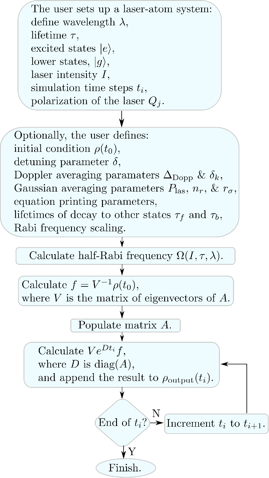
The process of setting up a laser-atom system and finding the solutions to the equations of motion is outlined in Fig. 1. LASED enables a user to define an atomic system by creating the states and substates of the atom that are coupled by the laser. Their relative energy separation, angular momenta, and the projection of the total angular momentum associated with each state are also input to the model as initial parameters. The substates are labelled as either an upper state $|{e}\rangle$ or a lower state $|{g}\rangle$. The resonant transition laser wavelength between upper and lower states is defined as $\lambda$. The user then enters the laser parameters by defining the laser polarization $Q$ and the intensity $I$. This sets up the initial laser-atom system to be solved. The time steps $t_{i}$ over which the simulation is run is also defined before the system evolves. At the initial time step $t=t_{0}$ the laser is turned on.

To solve the user-defined laser-atom system, equations 19, 20 and 21 are used to automatically generate the complete set of coupled differential equations which are solved numerically. LASED uses a matrix method by writing the equations in the form

$$\dot{\rho}=A\rho(t)$$

(29)

where $\rho$ is a column vector containing all the populations and coherences defined within the density matrix for the coupled system. The density matrix has $n^{2}$ elements, where $n$ is the number of substates in the system. $\rho$ is hence a column vector of $n^{2}$ elements. $A$ is an $n^{2}\times{n^{2}}$ coupling matrix that contains all of the coefficients of the interaction. This includes all half-Rabi frequencies generated from equation 23, the detuning terms and all decay constants. The matrix $A$ can become very large, and so to reduce computation time equation 29 is solved by diagonalising the matrix and calculating the eigenvectors and eigenvalues. The solution of $\rho$ using this technique then gives

$$\rho(t)=Ve^{Dt}V^{-1}\rho(t_{0})$$

(30)

where $A=VDV^{-1}$. $D$ is the diagonalised form of $A$ that contains the complex eigenvalues and $V$ is the matrix of eigenvectors of $A$. All real terms in the eigenvalues generated by the calculation must be negative for the solutions to converge. The initial condition $\rho(t_{0})$ can be defined by the user when setting up the laser-atom system. If the initial conditions are not defined by the user, it is assumed that all lower substates have equal populations and that all atomic coherences are identically zero prior to the laser being turned on (as would occur if the atomic beam was generated from an oven or from a gas jet).

Using this matrix method requires the populations and coherences to be in a strict order within $\rho$. The user hence has to define the substate with a number that labels it, e.g. $|{1}\rangle$, $|{2}\rangle$, and $|{3}\rangle$ for a lower $P$-state with ${m=-1,0,+1}$ respectively. The convention used throughout LASED is that the first element in the vector $\rho$ is the element $\rho_{11}$, which is the lower state population with the lowest projection of angular momentum $-m_{F}$. The labelling continues until the excited substate population with the largest projection of total angular momentum $+m_{F}$ is set to be the $n^{th}$ substate. The vector would hence have the form: [$\rho_{11}$ $\rho_{12}$ … $\rho_{1n}$, $\rho_{21}$ $\rho_{22}$ … $\rho_{2n}$, $\rho_{n1}$ $\rho_{n2}$ … $\rho_{nn}$]. The matrix $A$ is then populated using the coefficients generated using equations 19 to 21. These can be modified to give a set of equations with computable variables:

	$\displaystyle\dot{\rho}_{gg^{\prime\prime}}=$	$\displaystyle-(i\Delta_{gg^{\prime\prime}}+\frac{1}{\tau_{b}})\rho_{gg^{\prime\prime}}$
		$\displaystyle+i\Omega\sum_{qe}(C^{q}_{eg^{\prime\prime}}\rho_{ge}-C^{q}_{eg}\rho_{eg^{\prime\prime}})$
		$\displaystyle+\frac{1}{2\tau}\sum_{qe^{\prime}e^{\prime\prime}}\gamma^{q}_{e^{\prime}e^{\prime\prime}}\rho_{e^{\prime\prime}e^{\prime}}+\gamma^{q}_{e^{\prime\prime}e^{\prime}}\rho_{e^{\prime}e^{\prime\prime}}$		(31)

	$\displaystyle\dot{\rho}_{ee^{\prime\prime}}=$	$\displaystyle-(i\Delta_{ee^{\prime\prime}}+\frac{1}{\tau}+\frac{1}{\tau_{f}})\rho_{ee^{\prime\prime}}$
		$\displaystyle+i\Omega\sum_{qg}(C^{q}_{e^{\prime\prime}g}\rho_{eg}-C^{q}_{eg}\rho_{ge^{\prime\prime}})$		(32)

	$\displaystyle\dot{\rho}_{ge}=$	$\displaystyle-i(\Delta^{q}_{eg}+\delta+\frac{1}{2\tau}+\frac{1}{2\tau_{f}}+\frac{1}{2\tau_{b}})\rho_{ge}$
		$\displaystyle-i\Omega\sum_{qe^{\prime}}C^{q}_{e^{\prime}g}\rho_{e^{\prime}e}+i\Omega\sum_{qg^{\prime}}C^{q}_{eg^{\prime}}\rho_{gg^{\prime}}.$		(33)

The decay constants in $\dot{\rho}_{gg^{\prime\prime}}$ are contained in the term

		$\displaystyle\gamma^{q}_{e^{\prime}e^{\prime\prime}}=$
		$\displaystyle\begin{cases}\frac{|C^{q}_{e^{\prime}g^{\prime\prime}}C^{q}_{e^{\prime\prime}g}|}{\sum_{g^{\prime}}|C^{q}_{e^{\prime\prime}g^{\prime}}C^{q}_{e^{\prime}g^{\prime}}|},&\text{if $e^{\prime}=e^{\prime\prime}$}\\ \Gamma_{e^{\prime}ge^{\prime\prime}g},&\text{if $e^{\prime}\not=e^{\prime\prime}$ AND $\sum_{q}C^{q}_{e^{\prime}g}C^{q}_{e^{\prime\prime}g}\not=0$}.\end{cases}$		(34)

where the sum over $q$ is the sum of all values over which spontaneous emission can occur: +1, 0, and -1. The second case in equation 34 only appears when there is hyperfine splitting leading to vertical coherences Farrell et al. 1988.

The calculation of the generalized decay constants and their phase is shown in appendix B. The coupling coefficients are calculated using equation 5 and the maximum half-Rabi frequency $\Omega$ is calculated using equation 23. The detuning term is calculated using equation 22 as discussed in section II. The laser-atom system modelled using equations 31 to 33 are more general than the system modelled using equations 19 to 21 as these also include extra decay terms that describe the process of relaxation to states which are not directly coupled by the laser, as shown in Fig. 2. These include states that $|{e}\rangle$ and $|{g}\rangle$ may decay to that are not included in equations 19 to 21, as well as any non-radiative decay routes that may occur. The decay from a laser-excited state $|{e}\rangle$ to a non-coupled state $|{f}\rangle$ is modelled by the lifetime $\tau_{f}$ and the decay from a lower state $|{g}\rangle$ to a non-coupled state $|{b}\rangle$ is modelled by the lifetime $\tau_{b}$. Equation 33 also includes a detuning term $\delta$, which allows the user to add a constant detuning from resonance if required (e.g. for laser-cooling of atoms).

Whilst the matrix $A$ is being generated the equations of motion can be printed out in a numeric or symbolic format depending on the user’s preference. The Sympy package Meurer et al. 2017 is used to generate the symbolic equations, which can be output as LaTeX.

Once the matrix $A$ has been generated, the NumPy package Harris et al. 2020 is used to diagonalise the matrix to form $D$. NumPy is also used to perform all matrix multiplication in LASED. The SciPy package Virtanen et al. 2020 is used to generate the matrix of eigenvectors $V$ from $A$ and is also used in LASED to perform matrix exponentials and the inversion of matrices. For every element of the time array $t_{i}$ the column vector $\rho(t)$ of the laser-atom system is calculated numerically. Before looping over every element in $t_{i}$, $V^{-1}\rho(t_{0})$ is calculated to save computation time. During the loop over $t_{i}$, the matrix exponential $e^{Dt}$ is calculated by taking the exponent of each diagonal element of $Dt$. Finally, $\rho(t)$ is calculated using equation 30. Once the time evolution is completed, the user can access any element of $\rho(t)$ for analysis, the data can be saved as a csv file, or it can be plotted.

In this section the features of LASED are presented using examples from different laser-atom systems. For each simulation, the time evolution of the populations of various atomic substates is presented. The sum of the populations of all substates is initially set to unity and so the populations directly represent the probability of a particular atom in the ensemble being in that substate at any given time. Additional examples using LASED can be found at Patel 2021a.

References

- Neugart et al. (2017) R. Neugart, J. Billowes, M. Bissell, K. Blaum, B. Cheal, K. Flanagan, G. Neyens, W. Nörtershäuser, and D. Yordanov, Journal of Physics G: Nuclear and Particle Physics 44, 064002 (2017).
- Studer et al. (2019) D. Studer, S. Heinitz, R. Heinke, P. Naubereit, R. Dressler, C. Guerrero, U. Köster, D. Schumann, and K. Wendt, Physical Review A 99, 062513 (2019).
- Raab et al. (1987) E. Raab, M. Prentiss, A. Cable, S. Chu, and D. Pritchard, Physical Review Letters 59, 2631 (1987).
- Harvey and Murray (2008) M. Harvey and A. J. Murray, Physical review letters 101, 173201 (2008).
- Cortiñas et al. (2020) R. Cortiñas, M. Favier, B. Ravon, P. Méhaignerie, Y. Machu, J. Raimond, C. Sayrin, and M. Brune, Physical Review Letters 124, 123201 (2020).
- Urvoy et al. (2019) A. Urvoy, Z. Vendeiro, J. Ramette, A. Adiyatullin, and V. Vuletić, Physical review letters 122, 203202 (2019).
- Hertel and Stoll (1978) I. Hertel and W. Stoll, Advances in Atomic and Molecular Physics 13, 113 (1978).
- Farrell et al. (1988) P. Farrell, W. MacGillivray, and M. Standage, Physical Review A 37, 4240 (1988).
- MacGillivray and Standage (1988) W. MacGillivray and M. Standage, Physicals Reports 168, 1 (1988).
- Murray et al. (1989) A. Murray, C. Webb, W. MacGillvray, and M. Standage, Physical Review Letters 62, 411 (1989).
- Murray et al. (1990) A. Murray, W. MacGillivray, and M. Standage, Journal of Physics B: Atomic, Molecular and Optical Physics 23, 3373 (1990).
- Farrell et al. (1991) P. Farrell, W. MacGillivray, and M. Standage, Physical Review A 44, 1828 (1991).
- Murray et al. (1991a) A. Murray, W. MacGillvray, and M. Standage, Journal of Modern Optics 38, 961 (1991a).
- Murray et al. (1992) A. Murray, R. Pascual, W. MacGillivray, and M. Standage, Journal of Physics B: Atomic, Molecular and Optical Physics 25, 1915 (1992).
- Murray et al. (1991b) A. Murray, W. MacGillivray, and M. Standage, Physical Review A 44, 3162 (1991b).
- Masters et al. (1996) A. Masters, A. Murray, R. Pascual, and M. Standage, Physical Review A 53, 3884 (1996).
- Murray and Cvejanovic (2003) A. J. Murray and D. Cvejanovic, Journal of Physics B: Atomic, Molecular and Optical Physics 36, 4889 (2003).
- Hussey et al. (2007) M. Hussey, A. J. Murray, W. MacGillivray, and G. C. King, Physical Review Letters 99, 133202 (2007).
- Murray et al. (2008) A. J. Murray, W. MacGillivray, and M. Hussey, Physical Review A 77, 013409 (2008).
- Hussey et al. (2008) M. Hussey, A. Murray, W. MacGillivray, and G. King, Journal of Physics B: Atomic, Molecular and Optical Physics 41, 055202 (2008).
- Nixon and Murray (2011) K. L. Nixon and A. J. Murray, Physical Review Letters 106, 123201 (2011).
- Nixon and Murray (2014) K. L. Nixon and A. J. Murray, Physical Review Letters 112, 023202 (2014).
- Rudolph et al. (2020) J. Rudolph, T. Wilkason, M. Nantel, H. Swan, C. M. Holland, Y. Jiang, B. E. Garber, S. P. Carman, J. M. Hogan, et al., Physical review letters 124, 083604 (2020).
- McClelland and Kelley (1985) J. McClelland and M. Kelley, Physical Review A 31, 3704 (1985).
- Robertson et al. (2021) E. J. Robertson, N. Šibalić, R. M. Potvliege, and M. P. Jones, Computer Physics Communications 261, 107814 (2021).
- Stenholm (1986) S. Stenholm, Reviews of modern physics 58, 699 (1986).
- Milošević (2017) D. Milošević, Physical Review A 96, 023413 (2017).
- Eckel et al. (2022) S. Eckel, D. S. Barker, E. B. Norrgard, and J. Scherschligt, Computer Physics Communications 270, 108166 (2022).
- Patel (2021a) M. Patel, LASED documentation (2021a), https://lased.readthedocs.io/en/latest/.
- Loudon (2000) R. Loudon, The quantum theory of light (OUP Oxford, 2000).
- Ackerhalt and Eberly (1974) J. Ackerhalt and J. Eberly, Physical Review D 10, 3350 (1974).
- Kubo (1963) R. Kubo, Journal of Mathematical Physics 4, 174 (1963).
- Whitley and Stroud Jr (1976) R. M. Whitley and C. Stroud Jr, Physical Review A 14, 1498 (1976).
- Farrell and MacGillivray (1995) P. Farrell and W. MacGillivray, Journal of physics A: Math. Gen. 28, 209 (1995).
- Meurer et al. (2017) A. Meurer, C. P. Smith, M. Paprocki, O. Čertík, S. B. Kirpichev, M. Rocklin, A. Kumar, S. Ivanov, J. K. Moore, S. Singh, T. Rathnayake, S. Vig, B. E. Granger, R. P. Muller, F. Bonazzi, H. Gupta, S. Vats, F. Johansson, F. Pedregosa, M. J. Curry, A. R. Terrel, v. Roučka, A. Saboo, I. Fernando, S. Kulal, R. Cimrman, and A. Scopatz, PeerJ Computer Science 3, e103 (2017).
- Harris et al. (2020) C. R. Harris, K. J. Millman, S. J. van der Walt, R. Gommers, P. Virtanen, D. Cournapeau, E. Wieser, J. Taylor, S. Berg, N. J. Smith, R. Kern, M. Picus, S. Hoyer, M. H. van Kerkwijk, M. Brett, A. Haldane, J. F. del Río, M. Wiebe, P. Peterson, P. Gérard-Marchant, K. Sheppard, T. Reddy, W. Weckesser, H. Abbasi, C. Gohlke, and T. E. Oliphant, Nature 585, 357 (2020).
- Virtanen et al. (2020) P. Virtanen, R. Gommers, T. E. Oliphant, M. Haberland, T. Reddy, D. Cournapeau, E. Burovski, P. Peterson, W. Weckesser, J. Bright, S. J. van der Walt, M. Brett, J. Wilson, K. J. Millman, N. Mayorov, A. R. J. Nelson, E. Jones, R. Kern, E. Larson, C. J. Carey, İ. Polat, Y. Feng, E. W. Moore, J. VanderPlas, D. Laxalde, J. Perktold, R. Cimrman, I. Henriksen, E. A. Quintero, C. R. Harris, A. M. Archibald, A. H. Ribeiro, F. Pedregosa, P. van Mulbregt, and SciPy 1.0 Contributors, Nature Methods 17, 261 (2020).
- Welford et al. (1991) D. Welford, D. Rines, and B. Dinerman, Optics letters 16, 1850 (1991).
- Siegman (1986) A. E. Siegman, Lasers (University science books, 1986).
- Brink et al. (1963) D. Brink, G. Satchler, and M. Danos, Physics Today 16, 80 (1963).
- Biedenharn et al. (1981) L. C. Biedenharn, J. D. Louck, and P. A. Carruthers, Angular momentum in quantum physics: theory and application, Vol. 8 (Addison-Wesley Reading, MA, 1981).
- Lurio et al. (1964) A. Lurio, R. DeZafra, and R. J. Goshen, Physical Review 134, A1198 (1964).
- Risberg (1968) G. Risberg, Arkiv for Fysik 37, 231 (1968).
- Beijers et al. (1987) J. Beijers, S. Doornenbal, J. van Eck, and H. Heideman, Journal of Physics B: Atomic and Molecular Physics (1968-1987) 20, 6617 (1987).
- Bray (2020) I. Bray, private communication (2020).
- Kramida et al. (2021) A. Kramida, Yu. Ralchenko, J. Reader, and and NIST ASD Team, NIST Atomic Spectra Database (ver. 5.9), [Online]. Available: https://physics.nist.gov/asd [2022, March 28]. National Institute of Standards and Technology, Gaithersburg, MD. (2021).
- Rafac et al. (1999) R. J. Rafac, C. E. Tanner, A. E. Livingston, and H. G. Berry, Physical Review A 60, 3648 (1999).
- Udem et al. (2000) T. Udem, J. Reichert, T. Hänsch, and M. Kourogi, Physical Review A 62, 031801 (2000).
- Arimondo et al. (1977) E. Arimondo, M. Inguscio, and P. Violino, Reviews of Modern Physics 49, 31 (1977).
- Patel (2021b) M. Patel, LASED source code (2021b), https://github.com/mvpmanish/LASED.
- Python Software Foundation (2022) Python Software Foundation, Python downloads (2022), https://www.python.org/downloads/.