sympy2c: from symbolic expressions to fast C/C++ functions and ODE solvers in Python Journal: Astronomy and Computing
Abstract
Computer algebra systems play an important role in science as they facilitate the development of new theoretical models. The resulting symbolic equations are often implemented in a compiled programming language in order to provide fast and portable codes for practical applications. We describe sympy2c, a new Python package designed to bridge the gap between the symbolic development and the numerical implementation of a theoretical model. sympy2c translates symbolic equations implemented in the SymPy Python package to C/C++ code that is optimized using symbolic transformations. The resulting functions can be conveniently used as an extension module in Python. sympy2c is used within the PyCosmo Python package to solve the Einstein-Boltzmann equations, a large system of ODEs describing the evolution of linear perturbations in the Universe. After reviewing the functionalities and usage of sympy2c, we describe its implementation and optimization strategies. This includes, in particular, a novel approach to generate optimized ODE solvers making use of the sparsity of the symbolic Jacobian matrix. We demonstrate its performance using the Einstein-Boltzmann equations as a test case. sympy2c is widely applicable and may prove useful for various areas of computational physics. sympy2c is publicly available at https://cosmology.ethz.ch/research/software-lab/sympy2c.html .
1 Introduction
Computer Algebra Systems (CAS), such as Mathematica [1] and SymPy [2], play an important role in scientific disciplines such as mathematics and theoretical physics, as they facilitate the development of new or modified theories. Most often, the resulting equations are implemented in a compiled programming language in order to provide fast, robust and portable codes for practical applications.
In this paper, we describe sympy2c, a new Python package designed to bridge the gap between the symbolic development and the numerical implementation of a theoretical model. For this purpose, sympy2c translates symbolic equations implemented within the Python CAS SymPy to fast C/C++ code that can then be used from Python as an extension module.
The development of sympy2c started in the field of computational cosmology as part of the Python package PyCosmo 11 1 https://cosmology.ethz.ch/research/software-lab/PyCosmo.html [3, 4, 5]. The concept of the just-in-time compiler HOPE [6] preceded the development of sympy2c. Among other features, PyCosmo offers a fast solver for Einstein-Boltzmann equations, a large system of ODEs which describes the evolution of linear perturbations in the Universe [7, 8]. To improve the code structure of PyCosmo and to make the code generator available to a wider audience, we separated the code creation part from the other functionalities of PyCosmo and thus created the separate Python package sympy2c.
sympy2c extends the basic C/C++ code generation functionalities of SymPy, for example by supporting special functions, numerical integration, interpolation and numerical solution of ODEs. We particularly optimised the sympy2c code generator for high dimensional stiff ODEs with a sparse Jacobian matrix. A direct solver for general sparse linear systems is at the heart of the ODE solver and will be described below in detail. sympy2c is publicly available at https://cosmology.ethz.ch/research/software-lab/sympy2c.html.
This paper is organised as follows. In Section 2, we introduce the role of Python in scientific programming, performance related aspects and the role of sympy2c within this context. In Section 3, we give an overview of functionalities offered by sympy2c and how to use the library. We list resources to access the sympy2c package, its source code and documentation in Section 4. In Section 5, we discuss the implementation and optimization details of sympy2c. In Section 6, we demonstrate the performance of sympy2c. In Section 7, we summarise our conclusions.
2 Fast Scientific Computation with Python
Python is an interpreted, high-level, general-purpose programming language with a focus on readability and efficient programming. Nowadays, it plays an important role in many scientific disciplines. Factors for its success in science are its permissive open source license, its extendability using C/C++, and the availability of high-quality and easy-to-use scientific packages.
Fundamental packages such as numpy and scipy are featured in multidisciplinary scientific journals [9, 10]. Python libraries for machine learning, such as TensorFlow [11], PyTorch [12] and scikit-learn [13] are widely used [14].
Another important package is SymPy, an open source computer algebra system (CAS) written in Python. SymPy can be used directly as a Python library, and does not implement its own programming language. This allows extending SymPy in Python and using SymPy with other Python libraries, without the difficulties caused by crossing language barriers.
Python is, in particular, widely used in astrophysics. Examples include astropy [15, 16], a Python package for astronomy that counts more than 5800 citations at Web of Science22 2 https://clarivate.com/products/web-of-science/ as of March 2022, and the data processing pipelines of the Event Horizon Telescope [17], the LIGO observatory [18] and the Legacy Survey of Space and Time (LSST) [19]. We refer the reader also to the article [20] which provides an overview of the role of Python in astronomy and science.
Since Python is an interpreted and dynamically typed programming language, it offers great flexibility and supports an agile development process. This, however, also implies reduced speed and higher memory consumption during run-time, features that have an impact in many scientific applications.
To circumvent this, solutions to increase execution speed have been developed and can be classified as follows:
- 1.
Implementation of parts of the code in a lower level language, such as C/C++ or Rust, or binding Python to existing C/C++ code. For example, large parts of numpy [9] and scipy [10] consist of a thin Python layer on top of BLAS [21] and other established numerical libraries. Notable tools to simplify bindings between Python and lower level languages include Cython [22], swig [23], pybind11 [24], f2py [25] or PyO3.
- 2.
- 3.
Automatic translation of Python code to C/C++, as supported by Pythran [28].
The sympy2c package fits in the third category but, in contrast to the mentioned tools, creates C/C++ code from SymPy expressions rather than from existing Python functions. The package pyodesys [29] follows a similar approach to generate C/C++ code for evaluating the right hand side of an ODE and its Jacobian matrix. pyodesys delegates these functions to existing ODE solvers, such as pygslodeiv2 [30], which do not take sparsity into account. The function autowrap of SymPy allows compilation of expressions to different back-ends such as C or FORTRAN. However, autowrap does not generate code for integrals or ODEs without an explicit symbolic solution and was thus not sufficient to be used within PyCosmo [3, 4, 5]. sympy2c differs from the mentioned tools by offering a very fast ODE solver by considering sparsity in the Jacobian and by implementing routines for numerical integration and spline interpolation.
3 Functionalities
In this section, we describe and demonstrate the main functionalities of sympy2c. For a detailed documentation of the sympy2c API we refer to the sympy2c online documentation, available at https://cosmo-docs.phys.ethz.ch/sympy2c/. More details about the inner workings of sympy2c follow in Section 5.
3.1 Functions
The steps to create and use a function are as follows:
- 1.
We declare a function by providing the symbolic expression which the function should evaluate and the arguments the function takes.
- 2.
We declare an extension module and add this function to the module.
- 3.
We trigger the code generation process and the compilation of the created code.
- 4.
We import the compiled Python extension module.
- 5.
We can now call the declared C-Function as a function within this module from Python.
We demonstrate the usage pattern of sympy2c in Listing 1 where we create and use a Python extension module with a function to compute the volume of a cylinder given its height and radius :
- 1.
Line 4: Contrary to Mathematica, symbols are not first-class citizens in Python, thus we have to declare r and h.
- 2.
Line 6: This declares an extension module.
- 3.
Line 7: We declare a function named "volume_cylinder" which computes the value of h * pi * r ** 2 and takes the arguments r and h.
- 4.
Line 8: We add this function to the extension module
- 5.
Line 10: Here we trigger code generation and compilation of the generated code. We also import the generated extension module as imported_module.
- 6.
Line 12: Now the function named volume_cylinder is available as part of the imported_module module.
3.2 Integrals
An important feature of sympy2c is the creation of C/C++ code for the numerical computation of integrals. sympy2c offers a function Integral which takes an expression, the integration variable and expressions for the lower and upper integration limits. When used, for example within a sympy2c Function, sympy2c creates C/C++ code to compute a numerical approximation.
This is especially useful when a closed form of the anti-derivative is unknown or not computable by SymPy. Internally, sympy2c calls well-established QUADPACK [31] routines available in the GNU Scientific Library (gsl)[32]. These routines also support computation of indefinite integrals.
The function Integral from sympy2c returns a symbolic function which can be used as any other expression but will later be translated to a routine for the numerical approximation of the integral.
Listing 2 shows an example of how to compute the gaussian integral with sympy2c:
- 1.
Line 6: This defines the symbolic integral . t is the integration variable and the symbol oo is used by SymPy to represent .
- 2.
Line 7: We add the function gauss which computes the given integral and takes no arguments.
- 3.
Line 10: We call the function gauss from Python, this will now execute the numerical integration.
3.3 Cubic Spline Interpolation
Interpolation functions can be helpful to speed up numerical computations. sympy2c offers a function InterpolationFunction1D which will create C/C++ code to call spline interpolation from gsl. Such interpolation functions can also be used within the integrand or in the limits for numerical integration as presented previously in Section 3.2 or as a term in the right hand side of the symbolic representation of an ODE as introduced later in Section 3.4.
Listing 3 showcases how this is supported within sympy2c:
- 1.
Line 6: This declares an interpolation function with the given name. It can be used as any other symbolic function, e.g. sympy.sin. Right now this serves as a "place holder function" and the user must provide appropriate values for the actual interpolation of the compiled extension module (see Line 12).
- 2.
Line 7: We add the function f which uses the interpolation function and computes cos_approx(t ** 2).
- 3.
Line 12: After compilation and import, the module contains a function set_cos_approx_values (this name is derived from the name we specified in Line 6) to setup the interpolation. Here we provide the values for the values .
- 4.
Line 15: We check the impact of the interpolation on the actual result.
3.4 Ordinary differential equations
sympy2c also generates efficient code for the numerical solution of stiff and non-stiff ordinary differential equations using the LSODA33 3 LSODA is a variant of LSODE (Livermore Solver for Ordinary Differential Equations) with Automatic method switching algorithm [33]. LSODA automatically switches between the Adams-Bashford method [34] for non-stiff and the BDF44 4 Backward Differentiation Formula method [35] for stiff time domains.
We used this method to replace the existing hand-crafted BDF solver from PyCosmo to benefit from the robust and efficient step-size control as well as from the detection of stiffness and automatic adaption of the order of the two LSODA integrators.
To demonstrate this feature, we consider the Robertson problem [36, 37], a common example of a stiff equation describing the kinetics of an autocatalytic chemical reaction of three reactants with concentrations and . This problem is often used as a test problem to compare solvers for stiff ODEs. The equations for the Robertson problem are as follows:
where values for the reaction coefficients are given by , and .
Listing 4 shows how to implement this ODE using sympy2c:
- 1.
Lines 6–8: These are the Robertson ODE equations.
- 2.
Line 13: Declaration to compile the ODE solver with sympy2c. We provide a name for the ODE, the time variable, a list of state variables (here named lhs) and the list or right-hand-side expressions of the ODE.
- 3.
Lines 17–19: Declaration of initial values, time grid for evaluation and tolerance settings.
- 4.
Lines 21–24: Finally solve the ODE and print the results.
4 Usage
The sympy2c package is hosted on https://pypi.org/project/sympy2c and hence can be installed using pip install sympy2c.
The source code for sympy2c is publicly hosted at https://cosmo-gitlab.phys.ethz.ch/cosmo_public/sympy2c and licensed under GPLv3.
To reduce the package size and to avoid potential license conflicts, sympy2c will download and compile external C code, such as the GNU Scientific Library [32], during the first invocation. The documentation is available at https://cosmo-docs.phys.ethz.ch/sympy2c/ and https://cosmology.ethz.ch/research/software-lab/sympy2c.html
5 Implementation
In this section, we describe the main features of the implementation of sympy2c. Since the fast ODE solver is at the heart of sympy2c and was one of the major drivers when implementing the package, we present its optimization strategy in more detail.
5.1 Python Extension Modules
As mentioned in Section 2, Python can be extended using extension modules [38]. The purpose of this method is either to improve performance of critical parts of a program, or alternatively to use existing external C/C++ code.
Instead of implementing extension modules directly, programmers can use Cython [22] which is a super-set of the Python language adding support for optional type declarations for variables, function arguments and return values. The Cython project offers tools to translate Cython source code into C/C++, including the code required to interact with the Python interpreter. Furthermore, using Cython to implement extension modules helps to avoid errors due to reference counting of Python objects and the created code compiles on all major operating systems and plays well with all Python versions 2.6 without the need to adapt the original Cython source code.
sympy2c uses Cython and its tools internally to make the generated C/C++ code accessible from Python and to create code which is independent of changes between different Python versions or operating systems and compilers.
5.2 The fast ODE solver
Implicit solvers for stiff ODEs require to solve a linear equation involving the Jacobian matrix of the right hand side of the ODE at each time step. These systems are often sparse with a structure that depends on the interactions of the components of the ODE.
A commonly used tool to solve dense linear systems is the LUP decomposition [39] which factors a matrix as where is a lower triangular matrix, is an upper triangular matrix and is a permutation matrix. This decomposition takes operations for a matrix of size . Since for permutation matrices, solving can be performed efficiently by first solving and then . Since both and are lower (respectively upper) triangular matrices, both steps involve forward (respectively backward) substitutions only.
To solve such systems, LSODA uses LAPACK’s [40] routines dgetrf to compute the LUP decomposition of general matrices, and dgbtrf for banded matrices. LSODA does not support other sparse matrix structures. Due to the run-time complexity of , the LUP decomposition dominates the overall run-time of LSODA for larger systems with a non-banded Jacobian.
sympy2c is able to gain major speed improvements by replacing the dgetrf routine with a specialised and fast implementation which considers the a-priori known sparsity structure derived from the symbolic representation of the ODE.
5.2.1 Loop unrolling in the linear solver
As an introduction into the code generator, we ignore the permutations in the LUP decomposition, and first focus on an LU decomposition.
sympy2c unrolls loops appearing in the computation of the LU decomposition. To illustrate the idea, we assume an identity matrix and for a matrix
| (1) |
The first step of the LU decomposition of consists then of the following nested loops:
Using dedicated variables for the matrix entries instead of arrays, and unrolling the loops during code generation, the previous code can be transformed to
Since , sympy2c reduces the number of computations by generating
The first implementation using for loops and arrays required 14 integer additions, 14 integer comparisons and 31 floating point operations, whereas the last specialized implementation requires 11 floating point operations only and no integer additions or comparisons.
5.2.2 Permutation handling
In the above example, we ignored the matrix for permuting rows for the sake of simplicity. In practice however, permuting rows to implement partial pivoting is necessary to control numerical errors [39] and cannot be ignored. To check if we need to swap rows, the solver checks for every row if the corresponding element on the diagonal has a higher magnitude than the elements in the same column below the diagonal. If this is not the case, rows are swapped.
The mathematical formulation to detect swapping is
| (2) |
This challenges our approach, since the values of are updated during the LUP decomposition and cannot be efficiently computed in advance.
We use sympy2c within PyCosmo to solve the same system with varying parameters over and over again. Therefore, we implemented the following adaptive strategy to mitigate this problem:
- 1.
Try to solve the linear system with the optimized solver without pivoting. The specialised solver implements the necessary checks if permutations are required and falls back to a general solver if required. In this case we record required permutations.
- 2.
Afterwards, we generate and compile more optimized solvers for for recorded permutations .
- 3.
In the next run, the solver switches between the existing specialized solvers if feasible. In case changes in the parameters of the ODE require a previously not appearing permutation, we fall back to the general solver as in step 1 and record permutations.
- 4.
Continue with step 2.
Our experiments to solve the Einstein-Boltzmann equations with varying parameters have shown that only very few of the described iterations are required to capture the involved permutations. This is also the case for physically very unlikely parameter combinations which potentially can arise in MCMC sampling [41].
To reduce the number of permutations required, we relaxed the check above with a configurable security factor to
| (3) |
The motivation behind this change is that we assumed that numerical issues most likely arise if the affected matrix entries differ on different orders of magnitude. We used or in our experiments, and observed a reduction of row swaps without significant differences between computed ODE solutions.
To further speed up the fallback LUP solver, we implemented a variant which considers an a-priori known banded structure in the symbolic representation of the linear system. This avoids looping over known zero entries but at the cost of tracking band limits during matrix updates in the LUP algorithm. This functionality is useful in our applications, but can be switched off since it increases run-time in case the given system is not banded.
5.2.3 Splitting
Large systems can create C/C++ functions of several millions lines of code for the unrolled LUP solvers. This can challenge the optimizer of the compiler resulting in long compilation times and high memory consumption. Our approach to mitigate these issues is to split a linear system into uncoupled separate systems using Schur-complements:
- 1.
We split the matrix into blocks with square matrices and (which may have different sizes) and also split and accordingly:
(4) - 2.
Using block-wise Gaussian elimination, we can solve this system in two steps:
(5) (6)
The code generator can compute the involved matrices symbolically and finally create two smaller C/C++ functions instead of one larger function. sympy2c can apply this idea recursively to create more and smaller functions in the generated code.
Another benefit is that the fallback general LUP solver now operates on smaller systems. The solution time can thus be significantly less affected in case arising permutations are not considered already: instead of solving a system of size having run-time , splitting the system of size into two uncoupled systems of size reduces the run-time by a factor of 4.
The drawback of this approach is reduced pivoting: in the extreme case of splitting a matrix of size into uncoupled solvers, sympy2c would not consider pivoting at all. We did not experience precision issues in our experiments for reasonable block sizes.
5.3 Code generation optimizations
Since SymPy is implemented in Python, extensive symbolic manipulations performed by sympy2c can slow down the code generation process. This especially applies for larger ODE systems. Another factor affecting the run-time of code involving sympy2c is the involved compilation of the generated C/C++ code. To improve run-time in both cases, sympy2c extensively uses disk-based caches to avoid repetitive computations such that speed is significantly improved for following executions and for smaller modifications of symbolic expressions.
To improve the performance of symbolic inversion of matrices needed in the splitting approach, we replaced the inv function from SymPy by recursive application of the following equation for of size and quadratic matrices of size and of size
| (7) | ||||
| (8) |
6 Performance
6.1 Setup
To test the performance of sympy2c, we consider the numerical solution of the Einstein-Boltzmann equations [7, 8] implemented in PyCosmo [4, 3]. This is a system of first-order linear homogeneous differential equations describing the evolution of linear perturbations in the Universe. The overall structure of the equation system is of the form
| (9) |
where is a vector of perturbation fields, prime denotes derivative with respect to a time variable , and is a time dependent Jacobian matrix. Generally also depends on the wave number , so this equation needs to be solved for a vector of values.
These equations are crucial for accurate cosmological model predictions. The radiation fields, photons’ temperature and polarization and (massless) neutrinos’ temperature, need to be described as an infinite hierarchy of multipoles, which are truncated to finite sums of length to allow numerical solutions. Thus, the size of the ODE system depends on a parameter l_max which leads to a system of size . In practical cases, the resulting dimension of pertubation fields can be several hundreds. This large dimensionality in addition to the stiff nature of the equations make their fast numerical solution challenging. For a theoretical analysis of this system of equations we refer to [42].
We published time measurements for different variations of the Einstein-Boltzmann equations in [3]. Below, we focus on demonstrating and comparing the effects of the discussed optimizations. The presented time measurements were performed on the high performance computing cluster Euler at ETH Zurich. We allocated a full node equipped with an EPYC 7742 processor from AMD. Further, we measured timings five times for every configuration and always report the fastest of these runs.
As noted above, the system depends on the wave number . Higher values of increase oscillations in the solution, which enforce smaller step-sizes in LSODA, and thus lead to longer computation times.
We compare run-times of different and resulting in equations systems of size .
6.2 Time Measurements
- 1.
n is the size of the system.
- 2.
mode:
- (a)
full indicates that we disabled all optimizations and LSODA always uses the fallback general LUP solver.
- (b)
banded indicates that we disabled all optimizations and LSODA uses the fallback LUP solver with the optimizations for the banded structure of the Jacobian matrix as described before.
- (c)
optimized refers to using the optimized linear solver using unrolled loops and avoiding computations involving known zeros.
- (a)
- 3.
is the total time spent in the full LUP linear solver. This solver is used when the optimized solver is disabled (modes full and banded), or when the optimized solver encounters an unknown row permutations and switches to the fallback LUP solver (mode optimized). Reporting the value in optimized mode indicates that the fallback solver was not required during solving the ODE system.
- 4.
is the total time spent in the optimized linear solver.
- 5.
is the overall time required to solve the differential equation. In addition to the time spent in solving linear equations measured as resp. , this also includes time spent in the actual LSODA algorithm.
- 6.
S is the achieved speedup to solve the ODE. This factor describes the reduction in run time compared to the baseline mode full.
| n | mode | [s] | [s] | [s] | S |
|---|---|---|---|---|---|
| 38 | full | 1.00 | |||
| banded | 2.15 | ||||
| optimized | 7.41 | ||||
| 158 | full | 1.00 | |||
| banded | 1.80 | ||||
| optimized | 183.36 | ||||
| 308 | full | 1.00 | |||
| banded | 2.05 | ||||
| optimized | 716.66 |
Tables 1, 2 and 3 show that the optimized solver spends no measurable time in the fallback LUP solver, indicating that no row permutations were required to ensure numerical precision. The speed-up we achieved is almost independent of but significantly influenced by the size of the system.
We did not find any numerical difference in the computed solutions for the different linear solvers. This is not surprising since the different solvers just reduce the number of computations involving zeros and else run the same algebraic operations in the same order.
| n | mode | [s] | [s] | [s] | S |
|---|---|---|---|---|---|
| 38 | full | ||||
| banded | |||||
| optimized | |||||
| 158 | full | ||||
| banded | |||||
| optimized | |||||
| 308 | full | ||||
| banded | |||||
| optimized |
| n | mode | [s] | [s] | [s] | S |
|---|---|---|---|---|---|
| 38 | full | 1.00 | |||
| banded | 2.18 | ||||
| optimized | 8.70 | ||||
| 58 | full | 1.00 | |||
| banded | 1.66 | ||||
| optimized | 175.39 | ||||
| 158 | full | 1.00 | |||
| banded | 1.97 | ||||
| optimized | 691.24 |
6.3 Impact of the Fallback LUP solver
To trigger the use of the fall-back solver we had to choose . As shown in table 4, in this case the values in the column are non-zero in the optimized mode. The speed-up of the optimized solver is reduced significantly in this situation.
| n | mode | [s] | [s] | [s] | S |
|---|---|---|---|---|---|
| 38 | full | 1.00 | |||
| banded | 1.31 | ||||
| optimized | 2.53 | ||||
| 58 | full | 1.00 | |||
| banded | 1.79 | ||||
| optimized | 2.37 | ||||
| 158 | full | 1.00 | |||
| banded | 2.75 | ||||
| optimized | 3.85 |
Table 5 shows the execution time after updating and recompiling the generated C/C++ code based on the recorded row-permutations from the previous run. We can see that the optimized solver now achieves reduction in execution time similar to the measurements we presented before.
| n | mode | [s] | [s] | [s] | S |
|---|---|---|---|---|---|
| 38 | full | 1.00 | |||
| banded | 1.31 | ||||
| optimized | 7.53 | ||||
| 58 | full | 1.00 | |||
| banded | 1.79 | ||||
| optimized | 189.31 | ||||
| 158 | full | 1.00 | |||
| banded | 2.75 | ||||
| optimized | 881.80 |
6.4 Runtime scaling
We investigated the run-time scaling of the LSODA solver for different linear solvers as a function of the number of equations . Figure 5 shows how the run-time of both variants of the LUP solver (full and banded) grows similarly with , whereas the dependence on is flatter for the optimized solver.
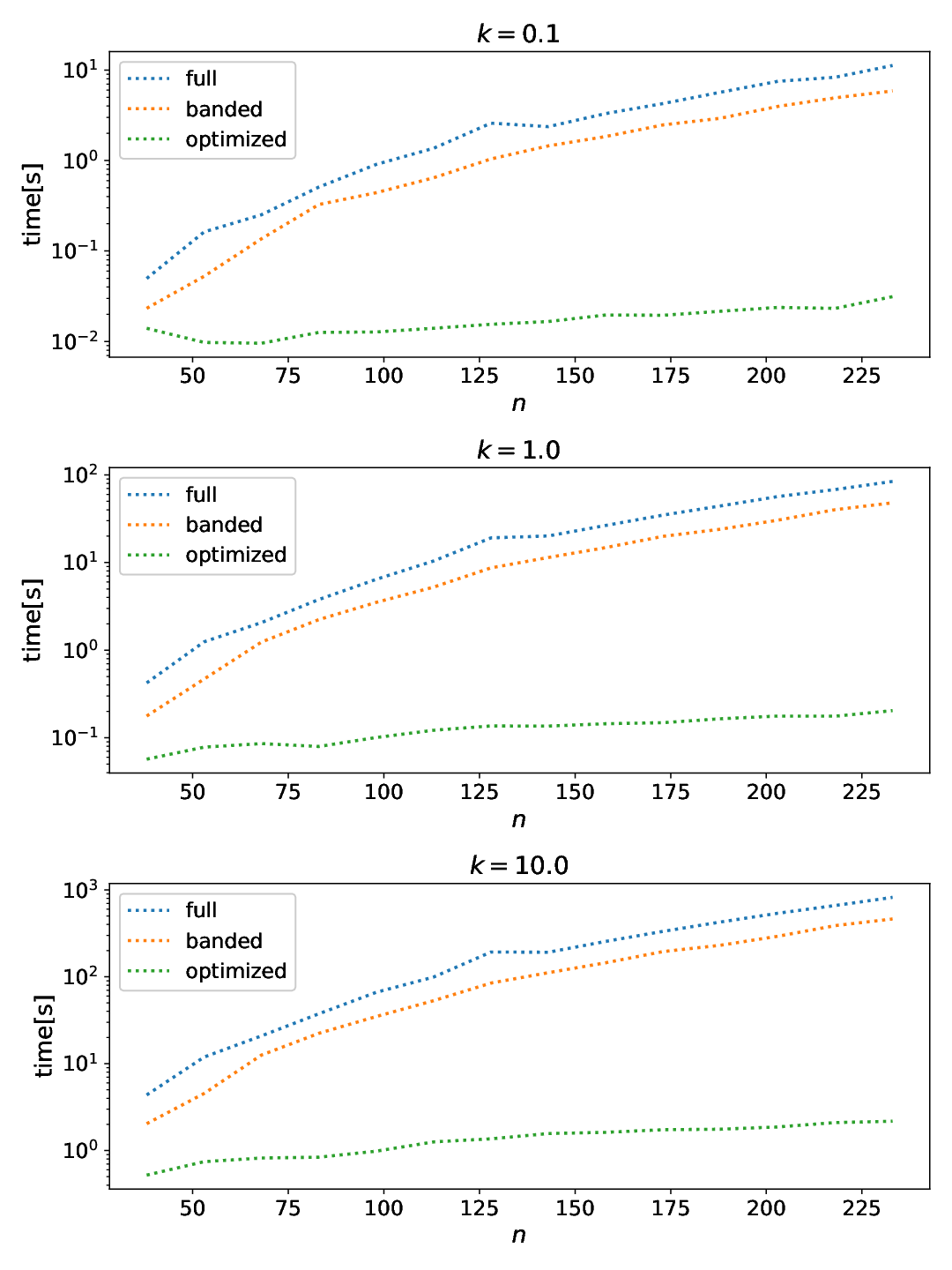
We performed polynomial fits of different orders and compared them using the AIC and BIC model selection criteria [43] using the Python package statsmodels [44]. We find that
- 1.
the run-times for solving systems of equations in the full and banded modes follow
(10) with fitted parameters and . The goodness of fit resulted in adjusted values for all values considered.
- 2.
the run-time for solving a system of equations in the optimized mode grows linearly in :
(11) with fitted parameters and . Fits achieved adjusted values for and for . Residuals for all appeared randomly distributed. This also indicates that the lower value for is caused by measurement noise and that there is no remaining term growing faster than which our fit may have missed.
Users of sympy2c thus benefit most from our optimized solver for large systems, but at the cost of upfront code generation and compilation times.
7 Conclusions
We presented the new sympy2c Python package for generating fast C/C++ code from symbolic expressions. sympy2c supports the creation of functions and solvers for stiff and non-stiff ordinary differential equations. It also implements functions to support numerical interpolation and integration. sympy2c is general and widely applicable and may thus prove useful for various areas of computational physics.
Our run-time measurements show that the optimization of the linear solver yield a significant improvement on the overall runtime performance of the ODE solver, in particular for larger systems. The overhead of code generation and compilation time limits application scope of the ODE solver to situations where the same ODE has to be solved many times with varying coefficients or initial conditions. To mitigate this, we plan to reduce the compilation times in future versions of sympy2c by creating more and smaller files to support the optimization step of the underlying compiler and to enable parallel compilation of different source code files.
8 Acknowledgements
The authors thank Joel Mayor for useful discussions on extensions of PyCosmo. This work was supported in part by grant No 200021_192243 from the Swiss National Science Foundation. sympy2c depends on the Python packages Cython [22] and sympy [2]. Further sympy2c makes use of the GNU Scientific Library (gsl)[32] and the LSODA source code [33]. Many ideas in sympy2c are influenced by the Python package HOPE [6] and previous developments in PyCosmo [4, 5].
Benchmarks were run on the Euler computing cluster at ETH Zurich55 5 https://scicomp.ethz.ch provided by the HPC team from Scientific IT Services of ETH66 6 https://sis.id.eth.ch.
References
- [1]
W. R. Inc., Mathematica, Version
12.3, champaign, IL (2021).
URL https://www.wolfram.com/mathematica - [2]
A. Meurer, C. P. Smith, M. Paprocki, et al.,
Sympy: symbolic computing in
python, PeerJ Computer Science 3 (2017) e103.
doi:10.7717/peerj-cs.103.
URL https://doi.org/10.7717/peerj-cs.103 - [3] B. Moser, C. S. Lorenz, U. Schmitt, et al., Symbolic Implementation of Extensions of the PyCosmo Boltzmann Solver (12 2021). arXiv:2112.08395.
- [4] A. Refregier, L. Gamper, A. Amara, L. Heisenberg, Pycosmo: An integrated cosmological boltzmann solver (2017). arXiv:1708.05177.
- [5] F. Tarsitano, U. Schmitt, A. Refregier, et al., Predicting cosmological observables with pycosmo (2020). arXiv:2005.00543.
- [6] J. Akeret, L. Gamper, A. Amara, A. Refregier, Hope: A python just-in-time compiler for astrophysical computations, Astronomy and Computing 10 (2015) 1–8.
- [7] C.-P. Ma, E. Bertschinger, Cosmological perturbation theory in the synchronous and conformal Newtonian gauges, Astrophys. J. 455 (1995) 7–25. arXiv:astro-ph/9506072, doi:10.1086/176550.
- [8] S. Dodelson, Modern Cosmology, Academic Press, Amsterdam, 2003.
- [9] C. R. Harris, K. J. Millman, S. J. van der Walt, et al., Array programming with numpy, Nature 585 (7825) (2020) 357–362.
- [10] P. Virtanen, R. Gommers, T. E. Oliphant, et al., Scipy 1.0: fundamental algorithms for scientific computing in python, Nature methods 17 (3) (2020) 261–272.
- [11]
T. Developers, Tensorflow,
Specific TensorFlow versions can be found in the "Versions" list on the
right side of this page.<br>See the full list of authors <a href="https://htt
ps://github.com/tensorflow/tensorflow/graphs/contr ibutors">on GitHub</a>.
(Jan. 2022).
doi:10.5281/zenodo.5898685.
URL https://doi.org/10.5281/zenodo.5898685 - [12]
A. Paszke, S. Gross, F. Massa, et al.,
Pytorch:
An imperative style, high-performance deep learning library, in: H. Wallach,
H. Larochelle, A. Beygelzimer, et al. (Eds.), Advances in Neural Information
Processing Systems 32, Curran Associates, Inc., 2019, pp. 8024–8035.
URL http://papers.neurips.cc/paper/9015-pytorch-an-imperative-style-high-performance-deep-learning-library.pdf - [13] F. Pedregosa, G. Varoquaux, A. Gramfort, et al., Scikit-learn: Machine learning in python, Journal of machine learning research 12 (Oct) (2011) 2825–2830.
- [14]
S. Raschka, J. Patterson, C. Nolet,
Machine learning in python:
Main developments and technology trends in data science, machine learning,
and artificial intelligence, Information 11 (4) (2020).
doi:10.3390/info11040193.
URL https://www.mdpi.com/2078-2489/11/4/193 - [15]
The Astropy Collaboration, Robitaille, Thomas P., Tollerud, Erik J.,
et al., Astropy: A
community python package for astronomy, A&A 558 (2013) A33.
doi:10.1051/0004-6361/201322068.
URL https://doi.org/10.1051/0004-6361/201322068 - [16]
A. M. Price-Whelan, B. M. Sipőcz, H. M. Günther, et al.,
The astropy project:
Building an open-science project and status of the v2.0 core package, The
Astronomical Journal 156 (3) (2018) 123.
doi:10.3847/1538-3881/aabc4f.
URL http://dx.doi.org/10.3847/1538-3881/aabc4f - [17] K. Akiyama, A. Alberdi, W. Alef, et al., First m87 event horizon telescope results. iii. data processing and calibration, The Astrophysical Journal Letters 875 (1) (2019) L3.
- [18]
B. P. Abbott, R. Abbott, T. D. Abbott, et al.,
Gw150914: First
results from the search for binary black hole coalescence with advanced
ligo, Phys. Rev. D 93 (2016) 122003.
doi:10.1103/PhysRevD.93.122003.
URL https://link.aps.org/doi/10.1103/PhysRevD.93.122003 - [19] M. Jurić, J. Kantor, K.-T. Lim, et al., The lsst data management system (2015). arXiv:1512.07914.
- [20]
D. Faes, Use of python
programming language in astronomy and science, Journal of Computational
Interdisciplinary Sciences 3 (3) (2012).
doi:10.6062/jcis.2012.03.03.0063.
URL http://dx.doi.org/10.6062/jcis.2012.03.03.0063 - [21] L. S. Blackford, A. Petitet, R. Pozo, et al., An updated set of basic linear algebra subprograms (blas), ACM Transactions on Mathematical Software 28 (2) (2002) 135–151.
- [22] S. Behnel, R. Bradshaw, C. Citro, et al., Cython: The best of both worlds, Computing in Science & Engineering 13 (2) (2011) 31–39.
- [23] D. M. Beazley, Swig: An easy to use tool for integrating scripting languages with c and c++, in: Proceedings of the 4th Conference on USENIX Tcl/Tk Workshop, 1996 - Volume 4, TCLTK’96, USENIX Association, USA, 1996, p. 15.
- [24] W. Jakob, J. Rhinelander, D. Moldovan, pybind11 – seamless operability between c++11 and python, https://github.com/pybind/pybind11 (2017).
- [25]
P. Peterson,
F2py:
a tool for connecting fortran and python programs, International Journal of
Computational Science and Engineering 4 (4) (2009) 296–305.
arXiv:https://www.inderscienceonline.com/doi/pdf/10.1504/IJCSE.2009.029165,
doi:10.1504/IJCSE.2009.029165.
URL https://www.inderscienceonline.com/doi/abs/10.1504/IJCSE.2009.029165 - [26] S. K. Lam, A. Pitrou, S. Seibert, Numba: A llvm-based python jit compiler, in: Proceedings of the Second Workshop on the LLVM Compiler Infrastructure in HPC, 2015, pp. 1–6.
- [27]
A. Rigo, S. Pedroni, Pypy’s
approach to virtual machine construction, in: Companion to the 21st ACM
SIGPLAN Symposium on Object-Oriented Programming Systems, Languages, and
Applications, OOPSLA ’06, Association for Computing Machinery, New York, NY,
USA, 2006, p. 944–953.
doi:10.1145/1176617.1176753.
URL https://doi.org/10.1145/1176617.1176753 - [28] S. Guelton, Pythran: Crossing the python frontier, Computing in Science Engineering 20 (2) (2018) 83–89. doi:10.1109/MCSE.2018.021651342.
- [29]
B. Dahlgren, pyodesys:
Straightforward numerical integration of ode systems from python, Journal of
Open Source Software 3 (21) (2018) 490.
doi:10.21105/joss.00490.
URL https://doi.org/10.21105/joss.00490 - [30] Bjorn, bjodah/pygslodeiv2: pygslodeiv2-0.9.4 (Apr 2020). doi:10.5281/zenodo.3760754.
- [31] R. Piessens, E. de Doncker-Kapenga, C. W. Überhuber, D. K. Kahaner, QUADPACK: A subroutine package for automatic integration, Vol. 1, Springer Science & Business Media, 2012.
- [32]
M. Galassi, GNU Scientific
Library : reference manual for GSL version 1.12, Network Theory, 2009.
URL http://www.worldcat.org/isbn/9780954612078 - [33] L. Petzold, Automatic selection of methods for solving stiff and nonstiff systems of ordinary differential equations, SIAM journal on scientific and statistical computing 4 (1) (1983) 136–148.
- [34] F. Bashforth, J. C. Adams, An attempt to test the theories of capillary action by comparing the theoretical and measured forms of drops of fluid, University Press, 1883.
- [35] C. F. Curtiss, J. O. Hirschfelder, Integration of stiff equations, Proceedings of the National Academy of Sciences of the United States of America 38 (3) (1952) 235.
- [36] H. Robertson, The solution of a set of reaction rate equations, Numerical analysis: an introduction 178182 (1966).
- [37] E. Hairer, G. Wanner, Solving ordinary differential equations. ii, volume 14 of (1996).
- [38] Extending Python with C or C++, https://docs.python.org/3/extending/extending.html.
- [39] H. Gene, C. F. Golub, Van loan. matrix computations third edition, Johns Hopikins Univ Pr (1996).
- [40] E. Anderson, Z. Bai, C. Bischof, et al., LAPACK Users’ Guide, 3rd Edition, Society for Industrial and Applied Mathematics, Philadelphia, PA, 1999.
- [41]
D. Foreman-Mackey, D. W. Hogg, D. Lang, J. Goodman,
emcee: The mcmc hammer, Publications
of the Astronomical Society of the Pacific 125 (925) (2013) 306–312.
doi:10.1086/670067.
URL http://dx.doi.org/10.1086/670067 - [42]
S. Nadkarni-Ghosh, A. Refregier,
The einstein–boltzmann
equations revisited, Monthly Notices of the Royal Astronomical Society
471 (2) (2017) 2391–2430.
doi:10.1093/mnras/stx1662.
URL http://dx.doi.org/10.1093/mnras/stx1662 - [43] K. Burnham, et al., dr anderson. 2002. model selection and multi-model inference: a practical information–theoretic approach, Ecological Modelling. Springer Science & Business Media, New York, New York, USA.
- [44] S. Seabold, J. Perktold, statsmodels: Econometric and statistical modeling with python, in: 9th Python in Science Conference, 2010.