Learning from All Vehicles

Dian Chen Philipp Krähenbühl Affiliation: UT Austin

Abstract

In this paper, we present a system to train driving policies from experiences collected not just from the ego-vehicle, but all vehicles that it observes. This system uses the behaviors of other agents to create more diverse driving scenarios without collecting additional data. The main difficulty in learning from other vehicles is that there is no sensor information. We use a set of supervisory tasks to learn an intermediate representation that is invariant to the viewpoint of the controlling vehicle. This not only provides a richer signal at training time but also allows more complex reasoning during inference. Learning how all vehicles drive helps predict their behavior at test time and can avoid collisions. We evaluate this system in closed-loop driving simulations. Our system outperforms all prior methods on the public CARLA Leaderboard by a wide margin, improving driving score by 25 and route completion rate by 24 points.

1 Introduction

Autonomous driving has been one of the most anticipated technologies since the advent of modern-day artificial intelligence. However, even after decades of exploration, we have yet to see self-driving cars deployed at scale. One main reason is the generalization. The world and its drivers are more diverse than current planning approaches can handle. Hand-designed classical planning Urmson et al. 2008; Leonard et al. 2008; Dolgov et al. 2008; Bacha et al. 2008 does not generalize gracefully to unseen or unfamiliar scenarios. Learning based methods Pomerleau 1989; Chen et al. 2015; Codevilla et al. 2018; Bansal et al. 2019; Chen et al. 2019 fare better, but suffer from a long tail of driving scenarios. The majority of driving data consist of easy and uninteresting behaviors. After all, humans drive thousands of hours before observing a traffic accident Tefft 2017, especially when driving an expensive autonomous test vehicle. How do we tame the long-tail of driving scenes? While many approaches rely on carefully crafted safety-critical scenarios in simulation Suo et al. 2021; Lopez et al. 2018; Peng et al. 2021, or collect massive data in the real world Bansal et al. 2019; Sun et al. 2020, in this paper we focus on an orthogonal direction.

Refer to caption — Figure 1: We present LAV, a mapless, learning-based end-to-end driving system. LAV takes as input multi-modal sensor readings and learns from all nearby vehicles in the scene for both perception and planning. At test time, LAV predicts multi-modal future trajectories for all detected vehicles, including the ego-vehicle. Picture credit – Waymo open dataset Sun et al. 2020.

We observe that, although many of us have not experienced traffic accidents ourselves, everyone has at least observed several accidents throughout our driving career. The same applies to safety-critical driving scenarios: While the data-collecting ego-vehicle might not experience accident-prone situations itself, it is likely its driving logs contain states that are interesting or safety-critical, but experienced by other vehicles. Training on other vehicles’ trajectories helps not only with sample efficiency, but also greatly increase the chance that the model sees interesting scenarios. Moreover, knowing other vehicles’ future trajectories helps the ego-vehicle avoid collisions.

The main challenge with training on all vehicles lies in the partial observability of other vehicles. Unlike the ego-vehicle, other vehicles have only partially observed motion trajectories, exposing no control commands or higher-level goals. This makes direct training Codevilla et al. 2018; Chen et al. 2019; Chen et al. 2021; Prakash et al. 2021; Chitta et al. 2021 on other vehicles’ traces close to impossible. More importantly, other vehicles have no accessible sensors. To learn from other vehicles, a model has to infer their surrounding state using the ego-vehicle’s sensors.

Our framework, Learning from All Vehicles (LAV), handles the partial observability of both perception and motion in one joint recognition, prediction, and planning stack. We decouple the partial observability challenge of perception and action using a privileged distillation approach Chen et al. 2019. LAV first learns a perception model that outputs a viewpoint invariant representation using auxiliary supervision from 3D detection and segmentation tasks. By definition, this auxiliary task does not distinguish between the ego-vehicle and other vehicles in the scene and thus learns a viewpoint invariant representation. It handles the partial observability of sensors. In parallel, LAV learns a privileged motion planner Chen et al. 2019. Instead of predicting steering and acceleration, which are only available for the ego-vehicle, we use future waypoints to represent the motion plan. We use ground-truth computer-vision labels as inputs to the privileged motion planner. Computer-vision labels ensure viewpoint invariance, waypoints provide an invariant representation of motion. The privileged motion planner predicts trajectories of all nearby vehicles and infers their high-level commands. Finally, we combine the two models in a joint framework using privileged distillation Chen et al. 2019. This final distillation learns a motion prediction model from all vehicles using the viewpoint invariant vision features of the perception model. The distilled policy drives from raw sensor inputs alone.

We validate our method in the CARLA driving simulator Dosovitskiy et al. 2017. At the time of submission, our method ranks first on the CARLA public leaderboard¹¹ 1 https://leaderboard.carla.org/leaderboard/. It attains a $\mathbf{61.85}$ driving score and a $\mathbf{94.46}$ route completion rate. Both are the highest among all methods and outperform the prior state-of-the-art method by a wide margin, increasing driving score and route completion rate by 25 and 24 points respectively. Our method won the 2021 CARLA Autonomous Driving challenge²² 2 https://ml4ad.github.io/. Code available at https://github.com/dotchen/LAV.

2 Related Work

Perception for autonomous driving

is driven by advances in visual understanding and recognition. The perception system of a self-driving vehicle understands the scene by inferring its nearby objects and surrounding road structures. A typical perception system takes as input LiDAR scans and performs object detection and tracking Zhou et al. 2020; Lang et al. 2019; Frossard et al. 2020; Zhou et al. 2020; Yin et al. 2021. Liang et al. 2018; Vora et al. 2020 fuse RGB camera and LiDAR scans for richer semantic information. For roads, perception systems are categorized based on whether they require pre-recorded HD-Map: map-based systems localize themselves in the pre-recoded maps Levinson et al. 2007; Zheng and Wang 2017; Ma et al. 2019; mapless systems either perform online mapping Garnett et al. 2019; Guo et al. 2020; Casas et al. 2021, or they implicitly predict road-related affordances Chen et al. 2015; Sauer et al. 2018; Toromanoff et al. 2020. Bansal et al. 2019; Zeng et al. 2019 represent the perception outputs as bird’s-eye-viewed (BEV) spatial grids; more recently, Gao et al. 2020; Li et al. 2021 represent perception outputs in a parameterized vector space for a more compact representation. Our approach takes multi-modal sensor data as input and performs online mapping and object detection. However, we do not directly use the predicted map to perform classical planning. Instead, we learn a planner from data using imitation learning. This planner uses every vehicle it encounters on the road as a supervisory signal to enhance the diversity of the training data.

Behavior prediction

focuses on forecasting the future state of driving scenes. In autonomous driving, a behavior predictor takes as either the input representations obtained from perception or raw sensor data; it predicts trajectories of the dynamic objects in the driving scene. Luo et al. 2018; Zeng et al. 2019 predict single, deterministic future trajectories of the detected vehicles. Zhao et al. 2020; Casas et al. 2018 model multi-modal future trajectories by using conditional models. Chai et al. 2019 predicts trajectories as Gaussian mixtures to represent uncertainty in the euclidean space. Lee et al. 2017; Cui et al. 2021 use latent variables and VAEs to model actor and scene specific uncertainties. Recently, Casas et al. 2021; Kamenev et al. 2021; Hu et al. 2021 combine perception and behavior prediction by directly predicting the occupancy maps. Our approach is highly related to the task of behavior prediction, as it also trains on all nearby vehicles’ trajectories. Our approach consists of a behavior predictor. In particular, it applies a conditional motion planner on all nearby vehicles, including the ego-vehicle.

Learning-based motion planning

uses imitation learning or reinforcement learning to plan future trajectories. Pioneered by Pomerleau 1989, imitation learning for autonomous driving regresses sensor inputs to controls by imitating the recorded expert trajectories. Codevilla et al. 2018 use conditional branching and high-level commands to extend imitative models for urban driving. Zeng et al. 2019 use imitation learning to train a cost volume predictor for planning; Chen et al. 2015; Sauer et al. 2018 predict actions from the learned affordances. Chen et al. 2019 uses on-policy distillation to handle distribution shift as well as to provide stronger imitative supervision signals. Reinforcement learning, on the other hand, trains policies from a user-defined reward function. Kendall et al. 2019 train a lane following driving policy using DDPG; Toromanoff et al. 2020 use distributed Rainbow-IQN to train an urban driving policy with competitive performance. Recently, Chen et al. 2021 use model-based reinforcement learning and distillation to train a driving policy in an offline manner. Our approach builds upon Chen et al. 2019 and trains a motion planner using imitation learning and distillation. However, unlike most prior methods, we train motion planning on data from all nearby vehicles in addition to the ego-vehicle.

Our idea of training the ego motion planner using data from all vehicles is closely related to Filos et al. 2021 and Zhang and Ohn-Bar 2021. Filos et al. 2021 extends offline reinforcement learning to learn from other agents’ behaviors. Zhang and Ohn-Bar 2021 train a privileged imitation learning policy that learns from other vehicles in a scene. Their policy side-steps partial observability by training a policy that acts only on the ground truth state of the simulator. It assumes perfect perception or access to other agents’ sensors. LAV, on the other hand, operates on raw sensor inputs and learns a viewpoint invariant intermediate representation.

3 Learning from All Vehicles

We aim to build a deterministic driving model $\pi$ that at each timestep $t$ maps sensor readings, high-level navigational command, and vehicle state to raw control command $a_{t}$ . We opt for an end-to-end differentiable three-stage modular pipeline: A perception module, a motion planner, and a low-level controller. See Figure 2(a) for an overview.

The perception module is trained from massive labeled supervision with two goals in mind: To create a robust and generalizable representation of the surrounding world, and to build vehicle-invariant features that help supervise the motion planner. Section 3.1 describes the overall architecture and training setup of the perception module. It maps raw sensor readings to a map-view feature representation.

The motion planner uses the map-view features of the perception model to produce a series of waypoints describing the future trajectory of the vehicles. Motion planners commonly use supervision from just the ego-vehicle for this prediction Chen et al. 2019. This supervision is quite sparse and provides the motion planner with just a single series of labels per collected data point. In our framework, we learn motion planning from all vehicles that surround the ego-vehicle. This is possible because our perception system produces vehicle-invariant features as inputs; it is also because the outputs of the motion planner, the future trajectories, can be easily obtained from ground truth driving logs. Figure 2(b) shows an overview of the motion planner training. Section 3.2 describes the motion planner and its training setup.

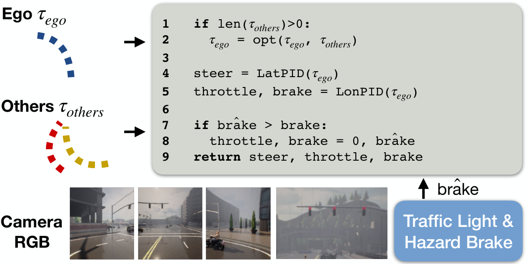
Finally, a low-level controller converts motion plans into actual steering and acceleration commands that are executed on the vehicle. At test time, the low-level controller considers other vehicles’ motion plans to make emergency stop decisions. Section 3.3 describes the controller.

3.1 A vehicle-independent perception model

The core objective of any perception module is to build an intermediate representation that readily generalizes from training to test conditions. In our setup, a secondary goal is to build input features to the motion planner that are indistinguishable between the current vehicle and nearby vehicles. The closer the output representations of the ego-vehicle and other vehicles are, the better motion plans transfer between those vehicles. Here, we opt for a metric map-based output representation. In a metric map, rotated ROI pooling extracts fixed-sized feature representations for training vehicles.

Specifically, we use three RGB cameras $\mathbf{I}_{t}=\{I_{t}^{1},I_{t}^{2},I_{t}^{3}\}$ surrounding the vehicle and one LiDAR sensor $L_{t}$ as an input. We combine the color and LiDAR inputs using point-painting Vora et al. 2020 from RGB inputs and a light-weight CenterPoint Yin et al. 2021 with PointPillars Lang et al. 2019 3D backbone. The backbone provides us with a map-view feature representation $f\in\mathbb{R}^{W\times H\times C}$ of width $W$ and height $H$ with $C$ channels.

We train the backbone network using a combination of semantic segmentation and detection losses. See Figure 3(a) for an overview. For every pixel in map-view, we predict a road mask, solid and broken lane boundaries. We use a binary classifier, and binary cross-entropy loss, as road and lane-marking can overlap. In addition, we train a CenterPoint-style detector Yin et al. 2021 for pedestrians and vehicles. Most importantly, we explicitly label the ego-vehicle in this detector. This minimizes the feature distance between ego-vehicle and other vehicles and enables better transfer. We pre-train the perception model using fully labeled data and use rotation augmentations around the ego-vehicle to increase the robustness of the learned model.

Supervised pre-training has two advantages. It generalizes better to unseen test conditions. It also learns a similar feature representation for all vehicles. This feature representation is next used in the motion planner.

3.2 Learning to plan motion from all vehicles

The motion planner uses the output of the perception system to predict a series of future waypoints describing positions the vehicles should steer towards. Here, we propose a novel two-stage motion planner that combines geometric GPS targets and discrete high-level commands. We use a standard RNN formulation Lee et al. 2017; Prakash et al. 2021 to predict $n=10$ future waypoints $y_{1},\ldots,y_{n}\in\mathbb{R}^{2}$ . We use $n=20$ for our second leaderboard submission. The motion planner uses a high-level command $c$ and intermediate GNSS coordinate goal $g\in\mathbb{R}^{2}$ to perform different driving maneuvers. In CARLA, GNSS goals are sampled every 50-100 meters and contain a measurement error of around one meter. Possible high-level commands $c$ include turn-left, turn-right, go-straight, follow-lane, change-lane-to-left, change-lane-to-right.

Let $M(\hat{f},c):\rightarrow\mathbb{R}^{n\times 2}$ be the motion planner conditioned on high-level command $c$ and warped features $\hat{f}$ for the Region of Interest (RoI) at the location and orientation of the vehicle in question. For all vehicles, we observe their future trajectory to obtain supervision for future waypoints $y$ . For the ego-vehicle, the simulator provides a ground truth high-level command $\hat{c}$ and provides sufficient supervision to train the motion planner

\displaystyle\mathcal{L}_{M}^{ego}=\mathrm{E}_{\hat{f},y,\hat{c}}\left[\|y-M(\hat{f},\hat{c})\|_{1}\right].

(1)

However, other vehicles do not expose their high-level commands. While it may be possible to infer this command from future trajectories alone, any rule-based inference will be ambiguous and noisy. We instead allow the model to infer the high-level command directly and optimize the plan for the most fitting high-level command.

\displaystyle\mathcal{L}_{M}^{other}=\mathrm{E}_{\hat{f},y}\left[\min_{c}\|y-M(\hat{f},c)\|_{1}\right].

(2)

At training time we optimize both losses $\mathcal{L}_{M}^{ego}$ and $\mathcal{L}_{M}^{other}$ jointly. To avoid mode collapse, we use an adaptive weight $\lambda$ on $\mathcal{L}_{M}^{other}$ which starts small and converges to 1 as training progresses. We found $\lambda=1-0.8^{it/4000}$ to work well in practice. This is only applied during the privileged training stage.

The resulting motion planner $M$ finds good coarse trajectories for a wide range of traffic scenarios. It learns to plan for all vehicles it sees. However, the resulting motion plan may be noisy as high-level commands $c$ are ambiguous.

In a second stage, we refine the motion plan using an additional RNN-based motion planning network $M^{\prime}(\hat{f},g,\tilde{y})\in\mathbb{R}^{n\times 2}$ . The motion refinement network uses the same ROI-warped feature $\hat{f}$ , the previously predicted motion plan $\tilde{y}$ , and the more fine-grain GNSS goal $g$ as input. We normalize $g$ in the ego-vehicle’s coordinate. It then produces a delta to the original trajectory as output. Since GNSS goals are only available for the ego-vehicle, we train the refinement $\hat{M}$ only on ego-vehicle trajectories

\displaystyle\mathcal{L}_{M}^{refine}=\mathrm{E}_{\hat{f},y,\tilde{y},\hat{g}}\left[\|\tilde{y}+M^{\prime}(\hat{f},\hat{g},\tilde{y})-y\|_{1}\right].

(3)

To increase robustness of the refinement model, we use the output of $M$ from all high-level commands during training. During both training and testing, we roll out the same refinement network multiple times to recursively refine the predicted trajectory. We use the refined trajectories for planning unless the high-level command is lane-changing. The above loss then applies to each step of the rollout.

In practice, we learn the motion planner in a privileged distillation framework Chen et al. 2019. See Figure 3(b) and Figure 3(c) for an overview. We first learn motion planning on ground truth trajectories and ground-truth perception outputs and regions of interest using the losses (1)-(3). We then use the privileged motion planner to supervise a motion planner that uses the inferred perception outputs. During this second stage, we supervise predictions on all high-level commands which leads to a richer supervisory signal Chen et al. 2019. We additionally distill a high-level command classifier for other vehicles which we use later in the vehicle-aware controller. This stage trains end-to-end by backpropagating gradients from motion prediction and planning to the perception backbone, allowing perception models to attend to the low-level details in the scenes. We keep the pre-training perception loss in the previous stage as an auxilliary supervision to regularize the features.

3.3 Vehicle-aware control

The controller translates a motion plan into actual driving commands. We use two PID controllers for latitudinal (steering) and longitudinal (acceleration) control. Both PID controllers use basic statistics of the refined motion plan as an input to produce a continuous output command. The longitudinal PID controller additionally uses the current speed as an input to compute acceleration. We overwrite braking using a separate neural network classifier $B$ in case of traffic light and hazard stoppages. The classifier uses the same image inputs as the perception module plus one additional camera with telephoto lenses to capture distant traffic lights. The classifier learns the braking behavior of the data-collecting ego-vehicle using recorded brake actions. Finally, we reuse the motion plans learned from other vehicles to detect potential collisions and perform hazard stops. Specifically, we use the 3D detections of the backbone to find all nearby vehicles. For each, we use the motion planner $M$ to produce future trajectories over each high-level command. We use all motion plans above the high-level command likelihood threshold to check for collisions with the ego-vehicle’s motion plan.

4 Implementation details

Perception.

We use PointPillars Lang et al. 2019 with PointPainting Vora et al. 2020 as our multi-modal 3D perception backbone $P_{B}$ . In particular, given RGB images captured from three frontal facing camera $\{I^{0}_{t},I^{1}_{t},I^{2}_{t}\}$ with extrinsic matrices $E=\{E^{0},E^{1},E^{2}\}$ , we use a ERFNet Romera et al. 2017 to compute their semantic segmentation scores $\mathbf{S}_{t}=\{S^{0}_{t},S^{1}_{t},S^{2}_{t}\}$ . We use five semantic classes: “background”, “vehicles”, “roads”, “lane markings” and “pedestrians”. For each LiDAR point $l\in L_{t}$ , we use PointPainting Vora et al. 2020 to concatenate its corresponding semantic classes using the segmentation scores: $l^{s}_{t}=\text{PointPaint}(\mathbf{S}_{t},\mathcal{T}_{E},l_{t})$ . $\mathcal{T}_{E}$ is the perspective transform function.

For PointPillars, we use FC-64-64 with BatchNorm Ioffe and Szegedy 2015 as its PointNet. We create pillars for LiDAR points for $x\in[-10\text{m},70\text{m}]$ and $y\in[-40\text{m},40\text{m}]$ . Each pillar represents a $0.25\text{m}\times 0.25\text{m}$ spatial region. We use the default 2D CNNs with multi-scale features to obtain the spatial features $\phi_{t}\in\mathbb{R}^{192\times 160\times 160}$ with $0.5\times$ resolution of the original pillars. Unlike the original PointPillars which directly builds dense pillars specified by the hyperparameters, we sparsely represent the pillars. We also use a sparse PointNet to process the corresponding sparse pillar features. This allows us to process all pillars efficiently both in space and time.

We use a branching architecture for the detection and mapping heads. We use a simplified one-stage CenterPoint Zhou et al. 2019; Yin et al. 2021 formulation for BEV object detection. In particular, we predict two “centerness” maps, one for vehicles and one for pedestrians; we also predict an orientation and bounding-box maps that are both class-agnostic. For mapping, we predict a BEV semantic map for roads, solid lane markings and broken lane markings. Each map is generated using a separate $3\times 3$ convolution followed by a $3\times 3$ up-convolution with stride $2$ , all from the shared backbone $P_{B}$ . At test time, we use a 2D max pooling layer as a simplified version of NMS.

We additionally train a binary brake classifier that takes as input all the four camera RGB images. We feed the telephoto lens image and the stitched other three images to a ResNet-18 followed by a global average pooling layer. This gives us fixed-sized embeddings of $z_{1},z_{2}\in\mathbb{R}^{512}$ . We concatenate $z_{1},z_{2}$ and feed it to a linear layer to predict the binary brake.

Prediction and Planning.

Given the ego-vehicle and a list of vehicle detection, we use differentiable warping to crop a rotated region of interest (RoI) $\hat{f}^{i}$ for each vehicle location and yaw angle. A CNN followed by global average pooling takes as input the rotated RoI features and returns a fixed-sized embedding $z^{i}$ for each vehicle $i$ . $z^{i}$ is shared among $M$ and $M^{\prime}$ . The motion planner $M$ uses a separate GRU Cho et al. 2016 for each high-level command. The GRU is rolled out $n$ times to produce an offset between consecutive waypoints. The refinement motion planner $M^{\prime}$ uses two forms of recursions and rollouts: rollouts along waypoint and rollouts along refinement iterations. It predicts an offset from the prior motion plan for each iteration. The refinement motion plan relies on just a single GRU unit that takes the GNSS goal $g$ as an additional input. Both motion planners use a linear layer to transform GRU states into the desired outputs.

Control.

The controller $C$ takes as input refined ego-trajectory $\tau=M^{\prime}(\hat{f},\tilde{y},\hat{g})$ . See Figure 4 for an overview. If predicted trajectory $\tau$ leads to a collision with other traffic participants, we adjust it. For now we perform a hard stop using a hard-coded braking logic. If the predicted trajectory is collision free, we follow it directly. We use two PID controllers for latitudinal and longitudinal control respectively. For latitudinal control, we use the $5$ -th point in $\tau_{5}$ as the aim point to compute the steering error. For longitudinal control, we use the difference between target speed inferred from $\|\tau_{k+1}-\tau_{k}\|$ and the current speed $v_{t}$ to compute acceleration. We use $K_{P}=1.0,K_{I}=0.5,K_{D}=0.2$ for the latitudinal PID controller, and we use $K_{P}=5.0,K_{I}=0.5,K_{D}=1.0$ for the longitudinal PID controller. We overwrite the brake control with the predicted brake score if it is larger than the brake computed from the longitudinal controller.

Rank	Method	Driving Score	Route Completion	Infraction Score
$1$	LAV	61.85	94.46	$0.64$
$2$	GRIAD Chekroun et al. 2021	$36.79$	$61.85$	$0.60$
$3$	TransFuser+ jae 2021	$34.58$	$69.84$	$0.56$
$4$	Rails Chen et al. 2021	$31.37$	$57.65$	$0.56$
$5$	IARL Toromanoff et al. 2020	$24.98$	$46.97$	$0.52$
$6$	NEAT Chitta et al. 2021	$21.83$	$41.71$	$0.65$
$7$	TransFuser Prakash et al. 2021	$16.93$	$51.82$	$0.42$
$8$	LBC Chen et al. 2019	$8.94$	$17.54$	0.73

Table 1: Comparison of the driving score (main metric), route completion and infraction score on the public CARLA leaderboard lea 2021 (accessed Jan 2022). All three metrics are higher the better. We outperform prior methods by a wide margin. Detailed infraction numbers reported in the supplement for reference.

	Driving Score	Route Completion	Infraction Score	Vehicle Collisions	Pedestrian Collisions	Layout Collisions	Red light Violations
LAV	$\textbf{45.20}\pm 6.35$	$\textbf{91.55}\pm 5.61$	$0.49\pm 0.06$	$\textbf{0.92}\pm 0.42$	$0.00\pm 0.00$	$\textbf{0.33}\pm 0.50$	$0.28\pm 0.28$
Ego-vehicle only	$38.56\pm 1.86$	$84.76\pm 5.12$	$0.46\pm 0.02$	$1.17\pm 0.50$	$0.00\pm 0.00$	$1.82\pm 0.06$	$0.34\pm 0.20$
No distillation	$28.23\pm 2.27$	$81.05\pm 6.04$	$0.36\pm 0.04$	$2.08\pm 0.34$	$0.00\pm 0.00$	$7.87\pm 0.15$	$\textbf{0.21}\pm 0.04$

Table 2: Driving performance ablation of the key components of our approach on test towns. Infractions are measured as number of occurrences per kilometer traveled. Mean and standard deviation are computed over three runs.

5 Experiments

We evaluate our method on the CARLA simulator Dosovitskiy et al. 2017 using closed-loop driving. We compare our approach with the state-of-the-art methods on the public leaderboard, and we perform ablation study on the effect of our design choices locally. For our online leaderboard submission, we train on all the 8 publicly available towns using a dataset of 400K frames, collected with the CARLA behavior agent under randomized weathers. For ablations, we only train on 4 out of the 8 towns, resulting in a dataset of 186K frames. We test on two other unseen towns.

More details of the dataset statistics are provided in the supplement for reference.

5.1 Comparison with state-of-the-art

Table 6 compares our method with prior state-of-the-art methods on the CARLA public leaderboard lea 2021. The CARLA leaderboard evaluates autonomous driving systems under unseen and partially adversarial conditions. Vehicles are tasked to complete a set of predefined routes in new towns. For each route, the simulator adds dangerous scenarios such as suddenly crossing pedestrians or aggressive lane-changing vehicles. These scenarios are modeled after the NHTSA typology lea 2021. The leaderboard measures how far self-driving vehicles proceed along a route within a fixed time budget, and how often they cause traffic infractions. In Table 6, we list three key metrics of the leaderboard: Driving Score, Route Completion, and Infraction Score. Route Completion measures the distance percentage an agent is able to complete; Infraction Score measures how often an agent drives without causing infractions; Driving Score measures route completion rate weighted by infractions per route. Driving Score and Route Completion are the two main metrics of comparison. A vehicle standing perfectly still will receive an infraction score of $1$ . All three metrics are higher the better. We refer readers to the official leaderboard lea 2021 for a more detailed description of the metrics.

We compare to the top 7 entries on the leaderboard. GRIAD Chekroun et al. 2021 and Transfuser+ are unpublished, concurrent submissions. Rails Chen et al. 2021 is a model-based reinforcement-learning method that trains vision-based driving policies from offline driving logs. IARL Toromanoff et al. 2020 is based on state-of-the-art model-free reinforcement-learning with distributed training. NEAT Chitta et al. 2021 uses imitation-learning with attention and implicit functions. Transfuser Prakash et al. 2021 uses imitation-learning with attention-based sensor fusion. LBC Chen et al. 2019 relies on knowledge distillation with imitation learning. LBC is the closest comparison to our approach, as we also use knowledge distillation and imitation learning as a supervisory signal. However, LAV additionally uses other observed vehicles to train the control policy.

LAV ranks first on the leaderboard, and it outperforms the prior leading entry by a wide margin. It achieves $\mathbf{61.85}$ driving score, the highest among all methods, and $\mathbf{25}$ points higher than on the previous state-of-the-art GRIAD. It also achieves a $\mathbf{94.46}$ Route Completion, the highest among all methods and $\mathbf{32}$ points higher than the previous state-of-the-art. Moreover, previous top methods, such as Rails and IARL, require 1M and 40M frames to train the policies. Our method uses only 400K training frames. Our approach has a relatively high infraction score; however, we note that higher Route Completion naturally leads to more infractions. A vehicle that drives slowly or stands still causes fewer infractions but struggles to complete its routes. See LBC for example.

5.2 Ablation study

We answer few important questions on our design choices. We again evaluate on Driving Score, Route Completion and Infraction Score. However, we cannot use the online leaderboard directly for these additional experiments. We instead use a local setup with similar characteristics to the Leaderboard. In particular, we train on 4 out of 8 towns (Town01, Town03, Town04 and Town06), and evaluate on 2 unseen towns (Town02 and Town05). We select 4 representative routes, 2 from each town, and we evaluate each route with 4 weathers: “Clear Noon”, “Cloudy Sunset”, “Soft Rain Dawn” and “Hard Rain Night”. We evaluate each setup for 3 runs and report the mean and standard deviation. This results in 48 trials for each model. All ablated models use a similar but slightly outdated setup as our leaderboard entry. The main differences are: 1. the ablated models use U-Net as the semantic segmentation backbone 2. the ablated models use FC-32-32 in PointPillars and 3. slightly different controller hyperparameters.

Table 2 studies the effects of our key design choices. We compare to two variants of our approach: 1) One that only trains on ego-vehicle data, 2) One that does not perform privileged distillation. We find that training on other vehicles’ trajectories and viewpoints results in lower performance on both route completion and infraction. The performance degradation is smaller than expected likely because our auxiliary perception supervision makes the motion models generalize well to distribution shifts, caused by both test time errors and viewpoints changes. Not using privileged distillation results in a larger performance drop. Without distillation, the motion models need to train from both noisy inputs and labels, thus tackling a much harder learning problem. Our full model achieves the highest scores in all three metrics.

Table 3 studies the degree to which training on other vehicles’ experiences affect the driving performance. We evaluate three standards, where we only train vehicles within 5, 15 and 25 meters within the ego-vehicle, with 15 meters being our default value. $\leq 5$ m and $\leq 15$ m performs equally well, while $\leq 25$ m is slightly worse. We think this is due to the fact that vehicles at range have too different of an appearance in the sensor inputs which the auxiliary supervision is unable to correct for. The LiDAR sensor in CARLA mimics the Velodyne-64 rays model, which produces at most a few dozen measurements for cars at a distance of $25$ m.

Table 4 studies different perception training schemes. We compare the default staged training scheme (staged) with two variants of joint training: 1) No perception pre-training (No Pretrain.), and joint perception and motion training (Joint). The first variant only optimizes the distillation loss, and the latter optimize perception and distillation simultaneously. Both variants do not freeze the 3D backbone. As expected, models without perception training perform poorly. They suffer from the distribution shifts caused by viewpoint changes. Joint training also performs worse than staged straining, because solving perception and planning simultaneously is harder than solving them in a disentangled manner, as also observed by Chen et al. 2019.

Table 5 studies the effect of our iterative refinement module. $K=0$ means we directly use the trajectories predicted by the motion planner $M_{f}$ to drive. The default option $K=5$ performs the best, showing the benefits of iterative motion refinement. Iterative refinement allows the model to elastically figure out what residuals to learn. It also naturally combines the semantic information from the high-level command and the geometric information from the goals.

Detailed infraction numbers for Table 3, Table 4 and Table 5 are provided in the supplement for reference.

Vehicles Range	Driving Score	Route Completion	Infraction Score
$\leq$ 5m	$\textbf{46.06}\pm 1.70$	$88.77\pm 1.01$	$0.51\pm 0.02$
$\leq$ 15m	$45.20\pm 6.35$	$\textbf{91.55}\pm 5.61$	$0.49\pm 0.06$
$\leq$ 25m	$37.42\pm 3.09$	$89.56\pm 5.61$	$\textbf{0.61}\pm 0.12$

Table 3: Driving performance in test towns of models trained with different range of other vehicles. All models are the same except for other vehicles’ maximum range used during training.

Perception Training	Driving Score	Route Completion	Infraction Score
No Pretrain.	$8.47\pm 0.83$	$9.34\pm 0.35$	$\textbf{0.90}\pm 0.07$
Joint	$28.36\pm 2.11$	$79.58\pm 4.99$	$0.34\pm 0.02$
Staged	$\textbf{45.20}\pm 6.35$	$\textbf{91.55}\pm 5.61$	$0.49\pm 0.06$

Table 4: Driving performance in test towns of models with different perception training scheme. All models are the same except for perception training.

Refinement Iteration	Driving Score	Route Completion	Infraction Score
$K=0$	$12.69\pm 2.86$	$35.85\pm 2.91$	$0.42\pm 0.03$
$K=1$	$21.30\pm 1.10$	$85.90\pm 2.46$	$0.25\pm 0.01$
$K=5$	$\textbf{45.20}\pm 6.35$	$\textbf{91.55}\pm 5.61$	$\textbf{0.49}\pm 0.06$

Table 5: Driving performance ablation on the effect of motion refinement. All models are the same except for number of refinement iterations.

5.3 Qualitative analysis

Figure 5 provides a qualitative analysis of our system. It shows the combined input images, LiDAR point cloud, the auxiliary segmentation predictions, detections, and predicted plans for all vehicles in the scene. The ego-vehicles plan uses the provided high-level command, while all other vehicles predict a distribution over possible future plans. Note how all vehicles predict a reasonable and consistent set of future plans aligning well with the inferred map-view representation of the road and the potential other vehicles.

6 Discussion

In this paper, we present a mapless, end-to-end driving system that trains from the experiences of all nearby vehicles. Our system achieves state-of-the-art performance in closed-loop driving simulation, and it outperforms prior leading methods by a wide margin. Limitations and potential negative social impacts: Our approach is trained and evaluated in simulation alone and still incurs traffic infractions. If directly deployed in the real world, it would most likely result in traffic accidents (negative social impacts). On the technical side, our current behavior predictor instantiated by the conditional motion planner does not consider multi-modality beyond the high-level commands. Extending our work with a probabilistic formulation will strengthen its ability in handling the diverse behaviors of both the ego vehicle and the other road users. Improving the motion predictor beyond its raster representation is also an exciting direction.

Acknowlegments

We thank Tianwei Yin for his help on pillar generation codes, Xingyi Zhou and Jeffrey Zhang for feedback on writing and figures. We thank TACC for providing part of our computing resources. This work was supported by the NSF Institute for Foundations of Machine Learning and NSF award #1845485.

References

lea (2021) Carla autonomous driving leaderboard (accessed november 2021). https://leaderboard.carla.org/leaderboard/, 2021.
jae (2021) Expert drivers for autonomous driving. urlhttps://kait0.github.io/files/master_thesis_bernhard_jaeger.pdf, 2021.
Bacha et al. (2008) Andrew Bacha, Cheryl Bauman, Ruel Faruque, Michael Fleming, Chris Terwelp, Charles Reinholtz, Dennis Hong, Al Wicks, Thomas Alberi, David Anderson, et al. Odin: Team victortango’s entry in the darpa urban challenge. Journal of field Robotics, 2008.
Bansal et al. (2019) Mayank Bansal, Alex Krizhevsky, and Abhijit Ogale. Chauffeurnet: Learning to drive by imitating the best and synthesizing the worst. RSS, 2019.
Casas et al. (2018) Sergio Casas, Wenjie Luo, and Raquel Urtasun. Intentnet: Learning to predict intention from raw sensor data. In CoRL, 2018.
Casas et al. (2021) Sergio Casas, Abbas Sadat, and Raquel Urtasun. Mp3: A unified model to map, perceive, predict and plan. In CVPR, 2021.
Chai et al. (2019) Yuning Chai, Benjamin Sapp, Mayank Bansal, and Dragomir Anguelov. Multipath: Multiple probabilistic anchor trajectory hypotheses for behavior prediction. In CoRL, 2019.
Chekroun et al. (2021) Raphael Chekroun, Marin Toromanoff, Sascha Hornauer, and Fabien Moutarde. GRI: general reinforced imitation and its application to vision-based autonomous driving. arXiv, 2021.
Chen et al. (2015) Chenyi Chen, Ari Seff, Alain Kornhauser, and Jianxiong Xiao. Deepdriving: Learning affordance for direct perception in autonomous driving. In ICCV, 2015.
Chen et al. (2021) Dian Chen, Vladlen Koltun, and Philipp Krähenbühl. Learning to drive from a world on rails. In ICCV, 2021.
Chen et al. (2019) Dian Chen, Brady Zhou, Vladlen Koltun, and Philipp Krähenbühl. Learning by cheating. In CoRL, 2019.
Chitta et al. (2021) Kashyap Chitta, Aditya Prakash, and Andreas Geiger. Neat: Neural attention fields for end-to-end autonomous driving. In ICCV, 2021.
Cho et al. (2016) Kyunghyun Cho, Bart van Merriënboer Caglar Gulcehre, Dzmitry Bahdanau, Fethi Bougares Holger Schwenk, and Yoshua Bengio. Learning phrase representations using rnn encoder–decoder for statistical machine translation. In EMNLP, 2016.
Codevilla et al. (2018) Felipe Codevilla, Matthias Müller, Antonio López, Vladlen Koltun, and Alexey Dosovitskiy. End-to-end driving via conditional imitation learning. In ICRA, 2018.
Cui et al. (2021) Alexander Cui, Sergio Casas, Abbas Sadat, Renjie Liao, and Raquel Urtasun. Lookout: Diverse multi-future prediction and planning for self-driving. In ICCV, 2021.
Dolgov et al. (2008) Dmitri Dolgov, Sebastian Thrun, Michael Montemerlo, and James Diebel. Practical search techniques in path planning for autonomous driving. In STAIR, 2008.
Dosovitskiy et al. (2017) Alexey Dosovitskiy, German Ros, Felipe Codevilla, Antonio Lopez, and Vladlen Koltun. Carla: An open urban driving simulator. In CoRL, 2017.
Filos et al. (2021) Angelos Filos, Clare Lyle, Yarin Gal, Sergey Levine, Natasha Jaques, and Gregory Farquhar. Psiphi-learning: Reinforcement learning with demonstrations using successor features and inverse temporal difference learning. arXiv preprint arXiv:2102.12560, 2021.
Frossard et al. (2020) Davi Frossard, Simon Suo, Sergio Casas, James Tu, Rui Hu, and Raquel Urtasun. Strobe: Streaming object detection from lidar packets. In CoRL, 2020.
Gao et al. (2020) Jiyang Gao, Chen Sun, Hang Zhao, Yi Shen, Dragomir Anguelov, Congcong Li, and Cordelia Schmid. Vectornet: Encoding hd maps and agent dynamics from vectorized representation. In CVPR, 2020.
Garnett et al. (2019) Noa Garnett, Rafi Cohen, Tomer Pe’er, Roee Lahav, and Dan Levi. 3d-lanenet: end-to-end 3d multiple lane detection. In CVPR, 2019.
Guo et al. (2020) Yuliang Guo, Guang Chen, Peitao Zhao, Weide Zhang, Jinghao Miao, Jingao Wang, and Tae Eun Choe. Gen-lanenet: A generalized and scalable approach for 3d lane detection. In ECCV, 2020.
Hu et al. (2021) Anthony Hu, Zak Murez, Nikhil Mohan, Sofía Dudas, Jeff Hawke, Vijay Badrinarayanan, Roberto Cipolla, and Alex Kendall. Fiery: Future instance prediction in bird’s-eye view from surround monocular cameras. In ICCV, 2021.
Ioffe and Szegedy (2015) Sergey Ioffe and Christian Szegedy. Batch normalization: Accelerating deep network training by reducing internal covariate shift. In ICML, 2015.
Kamenev et al. (2021) Alexey Kamenev, Lirui Wang, Ollin Boer Bohan, Ishwar Kulkarni, Bilal Kartal, Artem Molchanov, Stan Birchfield, David Nistér, and Nikolai Smolyanskiy. Predictionnet: Real-time joint probabilistic traffic prediction for planning, control, and simulation. arXiv preprint arXiv:2109.11094, 2021.
Kendall et al. (2019) Alex Kendall, Jeffrey Hawke, David Janz, Przemyslaw Mazur, Daniele Reda, John-Mark Allen, Vinh-Dieu Lam, Alex Bewley, and Amar Shah. Learning to drive in a day. In ICRA, 2019.
Lang et al. (2019) Alex H Lang, Sourabh Vora, Holger Caesar, Lubing Zhou, Jiong Yang, and Oscar Beijbom. Pointpillars: Fast encoders for object detection from point clouds. In CVPR, 2019.
Lee et al. (2017) Namhoon Lee, Wongun Choi, Paul Vernaza, Christopher B Choy, Philip HS Torr, and Manmohan Chandraker. Desire: Distant future prediction in dynamic scenes with interacting agents. In CVPR, 2017.
Leonard et al. (2008) John Leonard, Jonathan How, Seth Teller, Mitch Berger, Stefan Campbell, Gaston Fiore, Luke Fletcher, Emilio Frazzoli, Albert Huang, Sertac Karaman, et al. A perception-driven autonomous urban vehicle. Journal of Field Robotics, 2008.
Levinson et al. (2007) Jesse Levinson, Michael Montemerlo, and Sebastian Thrun. Map-based precision vehicle localization in urban environments. In RSS, 2007.
Li et al. (2021) Qi Li, Yue Wang, Yilun Wang, and Hang Zhao. Hdmapnet: An online hd map construction and evaluation framework. In CVPR Workshop, 2021.
Liang et al. (2018) Ming Liang, Bin Yang, Shenlong Wang, and Raquel Urtasun. Deep continuous fusion for multi-sensor 3d object detection. In ECCV, 2018.
Lopez et al. (2018) Pablo Alvarez Lopez, Michael Behrisch, Laura Bieker-Walz, Jakob Erdmann, Yun-Pang Flötteröd, Robert Hilbrich, Leonhard Lücken, Johannes Rummel, Peter Wagner, and Evamarie Wießner. Microscopic traffic simulation using sumo. In ITSC, 2018.
Luo et al. (2018) Wenjie Luo, Bin Yang, and Raquel Urtasun. Fast and furious: Real time end-to-end 3d detection, tracking and motion forecasting with a single convolutional net. In CVPR, 2018.
Ma et al. (2019) Wei-Chiu Ma, Ignacio Tartavull, Ioan Andrei Bârsan, Shenlong Wang, Min Bai, Gellert Mattyus, Namdar Homayounfar, Shrinidhi Kowshika Lakshmikanth, Andrei Pokrovsky, and Raquel Urtasun. Exploiting sparse semantic hd maps for self-driving vehicle localization. In IROS, 2019.
Peng et al. (2021) Zhenghao Peng, Quanyi Li, Ka Ming Hui, Chunxiao Liu, and Bolei Zhou. Learning to simulate self-driven particles system with coordinated policy optimization. In NeurIPS, 2021.
Pomerleau (1989) Dean A Pomerleau. Alvinn: An autonomous land vehicle in a neural network. In NeurIPS, 1989.
Prakash et al. (2021) Aditya Prakash, Kashyap Chitta, and Andreas Geiger. Multi-modal fusion transformer for end-to-end autonomous driving. In CVPR, 2021.
Romera et al. (2017) Eduardo Romera, José M Alvarez, Luis M Bergasa, and Roberto Arroyo. Erfnet: Efficient residual factorized convnet for real-time semantic segmentation. ITS, 2017.
Sauer et al. (2018) Axel Sauer, Nikolay Savinov, and Andreas Geiger. Conditional affordance learning for driving in urban environments. In CoRL, 2018.
Sun et al. (2020) Pei Sun, Henrik Kretzschmar, Xerxes Dotiwalla, Aurelien Chouard, Vijaysai Patnaik, Paul Tsui, James Guo, Yin Zhou, Yuning Chai, Benjamin Caine, et al. Scalability in perception for autonomous driving: Waymo open dataset. In CVPR, 2020.
Suo et al. (2021) Simon Suo, Sebastian Regalado, Sergio Casas, and Raquel Urtasun. Trafficsim: Learning to simulate realistic multi-agent behaviors. In CVPR, 2021.
Tefft (2017) Brian Tefft. Rates of motor vehicle crashes, injuries and deaths in relation to driver age, united states, 2014-2015. In AAA Foundation for Traffic Safety., 2017.
Toromanoff et al. (2020) Marin Toromanoff, Emilie Wirbel, and Fabien Moutarde. End-to-end model-free reinforcement learning for urban driving using implicit affordances. In CVPR, 2020.
Urmson et al. (2008) Chris Urmson, Joshua Anhalt, Drew Bagnell, Christopher Baker, Robert Bittner, MN Clark, John Dolan, Dave Duggins, Tugrul Galatali, Chris Geyer, et al. Autonomous driving in urban environments: Boss and the urban challenge. Journal of Field Robotics, 2008.
Vora et al. (2020) Sourabh Vora, Alex H Lang, Bassam Helou, and Oscar Beijbom. Pointpainting: Sequential fusion for 3d object detection. In CVPR, 2020.
Yin et al. (2021) Tianwei Yin, Xingyi Zhou, and Philipp Krahenbuhl. Center-based 3d object detection and tracking. In CVPR, 2021.
Zeng et al. (2019) Wenyuan Zeng, Wenjie Luo, Simon Suo, Abbas Sadat, Bin Yang, Sergio Casas, and Raquel Urtasun. End-to-end interpretable neural motion planner. In CVPR, 2019.
Zhang and Ohn-Bar (2021) Jimuyang Zhang and Eshed Ohn-Bar. Learning by watching. In CVPR, 2021.
Zhao et al. (2020) Hang Zhao, Jiyang Gao, Tian Lan, Chen Sun, Benjamin Sapp, Balakrishnan Varadarajan, Yue Shen, Yi Shen, Yuning Chai, Cordelia Schmid, et al. Tnt: Target-driven trajectory prediction. In CoRL, 2020.
Zheng and Wang (2017) Shuran Zheng and Jinling Wang. High definition map-based vehicle localization for highly automated driving: Geometric analysis. In ICL-GNSS, 2017.
Zhou et al. (2020) Xingyi Zhou, Vladlen Koltun, and Philipp Krähenbühl. Tracking objects as points. In ECCV, 2020.
Zhou et al. (2019) Xingyi Zhou, Dequan Wang, and Philipp Krähenbühl. Objects as points. arXiv preprint arXiv:1904.07850, 2019.
Zhou et al. (2020) Yin Zhou, Pei Sun, Yu Zhang, Dragomir Anguelov, Jiyang Gao, Tom Ouyang, James Guo, Jiquan Ngiam, and Vijay Vasudevan. End-to-end multi-view fusion for 3d object detection in lidar point clouds. In CoRL, 2020.

Appendix A Detailed Infractions

In this section we report additional infraction numbers of our experiments in the main manuscript. All infractions are measured as the number of occurrences normalized per $1$ kilometer traveled.

A.1 Comparison with state-of-the-art

Table 6 compares our method with baselines on the CARLA public Leaderboard lea 2021. Our method also leads the red light, offroad and blocked infraction numbers among all the methods.

Rank	Method	Driving Score	Route Completion	Infraction Score	Vehicle Collisions	Pedestrian Collisions	Layout Collisions	Red light Violations	Offroad Infractions	Blocked Infractions
$1$	LAV	61.85	94.46	$0.64$	$0.70$	$0.04$	0.02	0.17	0.25	0.10
$2$	GRIAD	$36.79$	$61.85$	$0.60$	$2.77$	0.00	$0.41$	$0.48$	$1.39$	$0.84$
$3$	TransFuser+	$34.58$	$69.84$	$0.56$	$0.70$	$0.04$	$0.03$	$0.75$	$0.18$	$2.41$
$4$	Rails Chen et al. 2021	$31.37$	$57.65$	$0.56$	$1.35$	$0.61$	$1.02$	$0.79$	$0.96$	$0.47$
$5$	IARL Toromanoff et al. 2020	$24.98$	$46.97$	$0.52$	$2.33$	0.00	$2.47$	$0.55$	$1.82$	$0.94$
$6$	NEAT Chitta et al. 2021	$21.83$	$41.71$	$0.65$	$0.74$	$0.04$	$0.62$	$0.70$	$2.68$	$5.22$
$7$	Transfuser Prakash et al. 2021	$16.93$	$51.82$	$0.42$	$1.09$	$0.91$	$0.19$	$1.26$	$0.57$	$1.96$
$8$	LBC Chen et al. 2019	$8.94$	$17.54$	0.73	0.40	0.00	$1.16$	$0.71$	$1.52$	$4.69$

Table 6: Comparison of our method and the state-of-the-art on the public CARLA leaderboard lea 2021 (accessed Jan 2022). Methods are ranked by the driving score as the main metric. Driving Score, Route Completion, Infraction Score are higher the better, whereas the rest are lower the better. Infractions are measured as number of occurences per kilometer traveled. We best all other methods by a wide margin. We significantly outperform the prior best entry by

\bf{24}

points on the driving score, and

\bf{25}

points on the route completion. We also lead the red light, offroad and blocked infraction numbers among all the methods.

Appendix B More Details

Town Name	Town Layout	Number of Frames
Town01	small, EU town	$46559$
Town02	small, EU town	$63564$
Town03	large, US town	$51896$
Town04	large, US town	$46244$
Town05	large, US town	$51489$
Town06	large, US town&highway	$41812$
Town07	small, US rural	$55465$
Town10	small, US city center	$42747$
Total		399776

Table 7: Number of frames and layouts of the training towns.

Figure 6 provdes an overview of architectures of $M$ and $M^{\prime}$ . We detach the gradient of coarse trajectories predicted by $M$ to remove any effect $M_{r}$ might have on $M_{f}$ during training.

Table 8 provides a list of hyperparameters. For all our experiments, we train our models on a 4 Titan Pascal GPU machine.

We use a ERFNet as our semantic segmentation architecture for PointPainting. We use the following image augmentations when we train the image-based semantic segmentation and brake prediction models: Gaussian Blur, Additive Gaussian Noise, Pixel Dropout, Multiply (scaling), Linear Contrast, Grayscale, ElasticTransformation.

B.1 Ablation study

Table 10 studies the effects of our key design choices. We additionally compare to a variant where we removes PointPainting Vora et al. 2020 (LiDAR only b.b.). The rest of the backbone is the same. Both Driving Score and Route Completion of this variant are lower than the full LAV. This shows the benefit of multi-modal sensor fusion. Table 11 studies the degree to which training on other vehicles’ experiences affect the driving performance. Table 12 studies different perception training schemes. Table 13 studies the effect of our iterative refinement module.

Note that our system does not rely on HD-Maps.

B.2 CARLA Leaderboard

Our online CARLA leaderboard entry additionally process temporal information by concatenating LiDAR scans normalized to the current vehicle pose. During training, this is done by stacking normalized frames using ground truth ego-vehicle poses. During testing, ego-vehicles poses are tracked across time via GNSS signals, smoothed by an Extended Kalman Filter (EKF) with a bicycle kinematics forward model. Following prior work Toromanoff et al. 2020, we use a “stuck counter” to avoid getting blocked. We creep forward if the vehicle is stuck for too long.

Stage	Hyperameter	Values
Privileged Motion	batch size	512
	learning rate	3e-4
	others weight $\lambda_{other}$	0.5
	command weight $\lambda_{cmd}$	0.1
Perception & Distill.	batch size	32
Perception & Distill.	learning rate	3e-4

Table 8: List of hyperparameters.

Appendix C Onboard Sensors

Table 9 provide a detailed description of the sensor configurations for the ego-vehicle. We use the compass readings from IMU and GNSS readings to convert the target locations, represented in the GNSS format, to the ego-vehicle coordinate.

Count	Modality	Shape	Note
$1$	LiDAR	$\mathbb{R}^{L\times 4}$	Velodyne-64
$1$	RGB	$\mathbb{R}^{3\times 288\times 480}$	FOV= $40^{\circ}$
$3$	RGB	$\mathbb{R}^{3\times 288\times 256}$	FOV= $64^{\circ}$ each $60^{\circ}$ apart
$1$	IMU	$-$
$1$	GNSS	$\mathbb{R}^{2}$
$1$	Speedometer	$\mathbb{R}$

Table 9: Configuration of our ego-vehicle’s on-board sensors. The four RGB cameras are mounted at

x=1.5\text{m},y=0\text{m},z=2.4\text{m}

with respect to the ego-vehicle’s centroid.

Appendix D Dataset Statistics

Table 7 describes the dataset statistics on the training towns and their corresponding layouts. Our online leaderboard submission trains on all towns, whereas our local ablation models train on Town01, Town03, Town04 and Town06. They test on Town02 and Town05.

Figure 7 provides a visualization of the four routes on which the ablation models are tested.

	Driving Score	Route Completion	Infraction Score	Vehicle Collisions	Pedestrian Collisions	Layout Collisions	Red light Violations	Offroad Infractions	Blocked Infractions
LAV	$\textbf{45.20}\pm 6.35$	$\textbf{91.55}\pm 5.61$	$\textbf{0.49}\pm 0.06$	$\textbf{0.92}\pm 0.42$	$0.00\pm 0.00$	$\textbf{0.33}\pm 0.50$	$0.28\pm 0.28$	$\textbf{0.27}\pm 0.01$	$\textbf{0.01}\pm 0.02$
Ego-vehicle only	$38.56\pm 1.86$	$84.76\pm 5.12$	$0.46\pm 0.02$	$1.17\pm 0.50$	$0.00\pm 0.00$	$1.82\pm 0.06$	$0.34\pm 0.20$	$0.37\pm 0.09$	$0.09\pm 0.08$
No distillation	$28.23\pm 2.27$	$81.05\pm 6.04$	$0.36\pm 0.04$	$2.08\pm 0.34$	$0.00\pm 0.00$	$7.87\pm 0.15$	$\textbf{0.21}\pm 0.04$	$1.01\pm 0.13$	$0.05\pm 0.05$
LiDAR only b.b.	$26.37\pm 2.62$	$74.96\pm 4.21$	$0.31\pm 0.04$	$6.51\pm 3.03$	$0.00\pm 0.00$	$0.02\pm 0.03$	$0.26\pm 0.23$	$1.56\pm 0.71$	$0.09\pm 0.04$

Table 10: Driving performance ablation of the key components of our approach on test towns. Infractions are measured as number of occurrences per kilometer traveled. Mean and standard deviation are computed over three runs. All models are the same despite the ablated option.

Vehicles Range	Driving Score	Route Completion	Infraction Score	Vehicle Collisions	Pedestrian Collisions	Layout Collisions	Red light Violations	Offroad Infractions	Blocked Infractions
$\leq$ 5m	$\textbf{46.06}\pm 1.70$	$88.77\pm 1.01$	$0.51\pm 0.02$	$1.27\pm 0.22$	$0.00\pm 0.00$	$\textbf{0.05}\pm 0.09$	$0.43\pm 0.11$	$0.69\pm 0.09$	$0.11\pm 0.10$
$\leq$ 15m	$45.20\pm 6.35$	$\textbf{91.55}\pm 5.61$	$0.49\pm 0.06$	$0.92\pm 0.42$	$0.00\pm 0.00$	$0.33\pm 0.50$	$0.28\pm 0.28$	$\textbf{0.27}\pm 0.01$	$\textbf{0.01}\pm 0.02$
$\leq$ 25m	$37.42\pm 3.09$	$89.56\pm 5.61$	$\textbf{0.61}\pm 0.12$	$\textbf{0.85}\pm 0.26$	$0.00\pm 0.00$	$0.61\pm 0.12$	$\textbf{0.23}\pm 0.13$	$0.43\pm 0.07$	$0.06\pm 0.10$

Table 11: Driving performance in test towns of models trained with different range of other vehicles. All models are the same except for other vehicles’ maximum range used during training.

Perception Training	Driving Score	Route Completion	Infraction Score	Vehicle Collisions	Pedestrian Collisions	Layout Collisions	Red light Violations	Offroad Infractions	Blocked Infractions
None	$8.47\pm 0.83$	$9.34\pm 0.35$	$\textbf{0.90}\pm 0.07$	$2.37\pm 2.08$	$0.00\pm 0.00$	$\textbf{0.00}\pm 0.00$	$\textbf{0.19}\pm 0.32$	$\textbf{0.15}\pm 0.26$	$\textbf{0.00}\pm 0.00$
Joint	$28.36\pm 2.11$	$79.58\pm 4.99$	$0.34\pm 0.02$	$1.65\pm 0.72$	$0.00\pm 0.00$	$7.75\pm 1.70$	$0.45\pm 0.32$	$0.49\pm 0.03$	$0.24\pm 0.21$
Staged	$\textbf{45.20}\pm 6.35$	$\textbf{91.55}\pm 5.61$	$0.49\pm 0.06$	$\textbf{0.92}\pm 0.42$	$0.00\pm 0.00$	$0.33\pm 0.50$	$0.28\pm 0.28$	$0.27\pm 0.01$	$0.01\pm 0.02$

Table 12: Driving performance in test towns of models with different perception training scheme. All models are the same except for perception training.

Refinement Iteration	Driving Score	Route Completion	Infraction Score	Vehicle Collisions	Pedestrian Collisions	Layout Collisions	Red light Violations	Offroad Infractions	Blocked Infractions
$K=0$	$12.69\pm 2.86$	$35.85\pm 2.91$	$0.42\pm 0.03$	$9.15\pm 3.88$	$0.00\pm 0.00$	$9.50\pm 2.02$	$0.33\pm 0.36$	$4.11\pm 2.11$	$1.41\pm 1.22$
$K=1$	$21.30\pm 1.10$	$85.90\pm 2.46$	$0.25\pm 0.01$	$2.09\pm 0.10$	$0.00\pm 0.00$	$5.58\pm 0.28$	$0.35\pm 0.26$	$0.93\pm 0.08$	$0.03\pm 0.03$
$K=5$	$\textbf{45.20}\pm 6.35$	$\textbf{91.55}\pm 5.61$	$\textbf{0.49}\pm 0.06$	$\textbf{0.92}\pm 0.42$	$0.00\pm 0.00$	$\textbf{0.33}\pm 0.50$	$\textbf{0.28}\pm 0.28$	$\textbf{0.27}\pm 0.01$	$\textbf{0.01}\pm 0.02$

Table 13: Driving performance ablation on the effect of motion refinement. All models are the same except for number of refinement iterations.

Appendix E License of Assets

We use the open source CARLA driving simulator Dosovitskiy et al. 2017. CARLA is released under the MIT license. Its assets are under the CC-BY license.

Our teaser figure in the main paper uses a picture from the Waymo open dataset Sun et al. 2020 The Waymo open dataset uses a customized non-commercial license³³ 3 https://waymo.com/intl/en_us/dataset-download-terms/. Part of our codebase uses the official ResNet and ERFNet implementation. The codes are under the MIT license and the CC-BY-NC license respectively.