Observation of Elastic Orbital Angular Momentum Transfer:
Coupling Flexural Waves in Partially Submerged Pipes to Acoustic Waves in FluidsPreprint: APS/123-QED
Abstract
Research into the orbital angular momentum carried by helical wave-fronts has been dominated by the fields of electromagnetism and acoustics, owing to its practical utility in sensing, communication and tweezing. Despite the huge research effort across the wave community, only recently has elastic orbital angular momentum been theoretically shown to exhibit similar properties. Here we experimentally observe the transfer of elastic orbital angular momentum from a hollow elastic pipe to a fluid in which the pipe is partially submerged, in an elastic analogue of Durnin’s slit-ring experiment for optical beams. This transfer is achieved by coupling the dilatational component of guided flexural waves in the pipe with the pressure field in the fluid; the circumferential distribution of the normal stress in the pipe acts as a continuous phased pressure source in the fluid resulting in the generation of Bessel-like acoustic beams. This demonstration has implications for future research into a new regime of orbital angular momentum for elastic waves, as well providing a new method to excite acoustic beams that carry orbital angular momentum that could create a new paradigm shift for acoustic tweezing.
Over the past three decades investigation into the orbital angular momentum (OAM) carried by helical waves has largely been reserved for light and sound Shen et al. 2019. The realisation by Allen et al. Allen et al. 1992 that electromagnetic Laguerre-Gaussian (LG) beams, satisfying the paraxial wave equation Fontaine et al. 2019, carry a well defined OAM sparked a resurgence in interest in exploiting this mechanical property of light for optical tweezers Yao and Padgett 2011; Loke et al. 2014; Allen et al. 2016; Padgett 2017; Barnett et al. 2017. The celebrated success of utilising LG beams comes, in part, from the ease in which they can be generated; a variety of simple devices can form these modes, for example spiral phase plates, q-plates, and spatial light modulators Higgins 1992; Oemrawsingh et al. 2004. The orbital angular momentum is associated with the spatial distribution of the beam, and not with the polarisation (that determines the intrinsic spin angular momentum) Allen et al. 1992; the inclined phase-fronts give rise to a well defined OAM about the beam axis that is proportional to the azimuthal index, or topological charge, . The azimuthal variation of phase forms a helical profile varying as , for azimuthal angle with the sign of determining the handedness of the helix. In general any optical beam with inclined phase fronts can carry a well-defined OAM O’Neil et al. 2002. Since this realisation other forms of optical beams that carry OAM have been investigated, by interference and superposition, such as higher-order Bessel beams McGloin et al. 2003; Vasilyeu et al. 2009, and more general vortex structures (knots) with non-integer OAM Leach et al. 2004; Leach et al. 2005; Götte et al. 2008; Morgan et al. 2017.
Translations of the phenomena surrounding OAM beams have been shown to hold for sound Bliokh and Nori 2019, with the transfer of torque for scalar waves within the non-paraxial regime being considered Zhang and Marston 2011; Zhang 2018. Similar applications in acoustic tweezers exist for micro-scale biological manipulation and communication, to name a few Hong et al. 2015; Baresch et al. 2016; Shi et al. 2017; Marzo et al. 2018. Conventionally the excitation of acoustic OAM modes rests on acoustic analogues of phase plates Hefner and Marston 1998; Hefner and Marston 1999, resonant devices and antenna concepts Jiang et al. 2016; Naify et al. 2016; Guo et al. 2019, or by discrete phased arrays Gibson et al. 2018; Antonacci et al. 2019; Cromb et al. 2020. Utilising discrete phased arrays is indeed a favoured method for the excitation of higher-order OAM acoustic modes, that carry topological charge Marchiano and Thomas 2005. Importantly, such higher-order modes exhibit an instability phenomenon: a vortex of charge is not stable and degenerates into vortices (screw dislocations) of charge Basistiy et al. 1993; Zambrini and Barnett 2006; Allen et al. 2016.
Recently the consideration of OAM has been extended further into the realm of elasticity, where both the spin-phonon coupling in elastic media and the intrinsic spin of elastic waves have been investigated Nakane and Kohno 2018; Long et al. 2018. The orbital angular momentum associated with only the compressional potential of flexural waves in elastic pipes has also been considered Chaplain et al. 2022, with the complete theory shown by Bliokh Bliokh 2022, proving that the total angular momentum (the sum of spin and orbital contributions) is quantised, as in electromagnetism and acoustics. In this paper we experimentally verify the experiment proposed in Chaplain et al. 2022, showing that the elastic OAM associated flexural waves can be coupled to a fluid, thereby observing its transfer through the excitation of acoustic pressure fields that carry OAM. Guided ultrasonic modes in pipes are considered, specifically flexural modes with a natural circumferential variation of phase. The coupling to the acoustic pressure in a fluid is achieved by partially submerging one end of the pipe in the fluid, in a set up resembling an elastic analogue of Durnin’s slit-ring experiment Durnin et al. 1987; Vasilyeu et al. 2009. We show that the generation of Bessel-like, higher-order acoustic OAM modes is possible, with clear agreement between simulation and experiments, highlighting specifically the features associated for an topological charge. Before introducing the flexural modes and the pipe structure we recall the governing equations of elastic materials and the associated compressional OAM.
An isotropic, homogeneous linear elastic material supports waves governed by the Navier-Cauchy equations Landau and Lifshitz 1959, following the Einstein summation convention,
| (1) |
and the constitutive law
| (2) | ||||
with the displacement and its double time derivative; Lamé’s first and second parameters are denoted , respectively with being the material density; and are the stress and stiffness tensors respectively; and is the strain tensor (comma notation denotes partial differentiation, and ).
The displacement comprises both shear and compressional motion, described by an equivoluminal vector potential and scalar dilatational potential respectively such that, by Helmholtz decomposition, . Elastic waves with inclined phase-fronts naturally occur as flexural modes in pipe walls Chaplain et al. 2022. Choosing cylindrical coordinates oriented with along the pipe axis the potentials take the form
| (3) | ||||
where . is the wave number along the pipe axis and the radian frequency. Stress free boundary conditions are imposed on the inner and outer radii , respectively, such that , along with the infinite cylinder gauge condition . The resulting radial distribution of the dilatational and shear potentials ( and ) are then described by a linear combination of Bessel functions and their modifications Gazis 1959a. We consider the coupling of elastic waves in a pipe with pressure fields in a fluid that the pipe is partially submerged. At the solid-fluid boundary the acoustic pressure induces a fluid load on the solid structure, and the structural acceleration acts as a normal acceleration across the solid-fluid boundary. The boundary conditions then manifest as the dynamic continuity of traction, and the kinematic continuity of the normal particle displacement at the interface between the solid and fluid, such that Morand and Ohayon 1995
| (4) | ||||
where is the acoustic pressure, is the unit tensor, is the particle displacement in the fluid and is the surface normal. In the fluid domain the governing equations follow the standard linearised Euler equations. For harmonic motion these read
| (5) | ||||
for fluid density with the acoustic wavespeed in the fluid denoted . The coupling boundary conditions of the elastoacoustic problem can then be expressed in the pure displacement formulation Bermúdez et al. 2008:
| (6) | ||||
These equations are solved numerically throughout via the Finite Element Method (FEM) COMSOL 2021.
The vector system of elasticity supports two body waves, compression and shear, that travel with distinct wavespeeds given by and respectively. Clearly, in the fully coupled elastic system, longitudinal (compressional), transverse (shear) and hybrid components all contribute to the orbital angular momentum, and thus to the total angular momentum (orbital and spin) Bliokh 2022. Therefore, the splitting of the displacement vector into the dilatational and shear potentials, as done in Chaplain et al. 2022, is not required; however, only considering the OAM associated with the compressional potential (that is proportional to the azimuthal index ) motivated this experimental work as fluids only support compressional waves and not shear.
Optical and acoustic tweezing are primary applications for the transfer of OAM, where particles can be trapped and manipulated at the vortex singularity at the beam centre Franke-Arnold et al. 2008; Hong et al. 2015. In the case of elastic OAM carried by flexural modes in pipes there is no such singularity as the pipe is hollow - a direct analogy cannot be drawn in this case as there is no elastic medium to suspend particles with at the pipe centre, along its axis. However, it is well known that vibrating solids radiate sound waves in fluids, and it is this coupling we leverage to excite an acoustic OAM mode via the flexural displacement field carried in the elastic pipe. We experimentally validate this OAM transfer, thereby developing a new continuous-phased acoustic source in the form of flexural modes in pipes; Bessel-like beams are generated following from the radial distribution of the compressional potential.
We first detail the background of flexural modes in pipes and how they are efficiently generated, using an elastic analogue to optical spiral phase plates. We utilise this analogue, the so-called elastic spiral phase pipe Chaplain and De Ponti 2022, to show the first experimental observation of the transfer of elastic OAM from flexural modes in pipes to fluids. We include qualitative comparisons with both Finite Element Method (FEM) simulations and Dynamic Mode Decomposition (DMD), and a comparison to classical discrete phased sources, before concluding and highlighting perspectives for applications.
Guided Flexural Modes in Pipes
Guided ultrasonic waves in pipes have long been studied, with the first analytical description being posed by Gazis in the late 1950s Gazis 1959a; Gazis 1959b, for infinitely long pipes. They fall into three modal classes: longitudinal (), torsional (), and flexural (), with a naming convention attributed to Silk and Bainton Silk and Bainton 1979 such that they are written , and . The integers , denote the circumferential and group order respectively; the circumferential order being analogous to the topological charge of optical vortex beams. The generation and inspection of these guided waves has found much success in non-destructive techniques and evaluation Alleyne et al. 1998; Lowe et al. 1998. The focus of this paper is to observe the coupling between non-axisymmetric flexural modes in pipes and acoustic waves in a fluid. As such we require a device to ensure their efficient generation.
The recent advent of the elastic spiral phase pipe (eSPP) Chaplain and De Ponti 2022 achieves this. This structure removes the necessity to rely on conventional means of complex arrangements of transducers or phased arrays (e.g by comb arrays or non-axisymmetric partial loading Shin and Rose 1999; Tang and Wu 2017). Advantages of the eSPP include passively exciting arbitrary flexural modes with, crucially, single handedness (i.e. only one sign of ) by mode converting longitudinal modes (e.g. ) that can be easily to excited in isolation Lowe 2001. This is a particularly attractive property as a candidate for using flexural modes that are sensitive to axial cracks, where the conventional longitudinal and torsional modes are weakly sensitive Kwun et al. 2008; Ratassepp et al. 2010.

In Fig. 1 we detail the eSPP used in the experimental verification of the transfer of elastic OAM. In Fig. 1(a) we show the elastic spiral phase pipe that endows incoming axisymmetric waves with a helical phase profile, similar to OAM generation by optical and acoustic analogues Beijersbergen et al. 1994; Hefner and Marston 1998; Hefner and Marston 1999. The spiral pipe used here has already been characterised Chaplain and De Ponti 2022, comprising an aluminium pipe of density , Young’s Modulus and Poisson’s ratio . The inner and outer diameters of the pipe are and respectively. One end of the pipe is open (to be submerged in fluid), while the other is capped with an aluminium disk of diameter and thickness , attached by six screws. The total length of the pipe is . The spiral region of the pipe is specifically designed to convert modes to modes at , and is formed of by CNC milling a thickness of from the pipe into three spiral steps of length . This step profile is determined via the method in Chaplain and De Ponti 2022, where an effective refractive index relates the two speeds of the incoming and converted waves through
| (7) |
where is again the modal index of the desired flexural mode (, here) and is the ratio of the wavespeeds of the converted flexural and incident longitudinal waves respectively, with the wavenumber of the incident mode along the pipe axis. To reduce the length of the step size the spiral is partitioned into three turns such that . The wavespeeds of each mode are determined through the dispersion of the pipe, evaluated by spectral collocation Adamou and Craster 2004; Chaplain and De Ponti 2022.
Transfer of Elastic OAM
To experimentally confirm the transfer of elastic OAM, we consider the coupling of the compressional component of a guided flexural mode in an elastic pipe, to the acoustic pressure field in a fluid (water) in which the pipe is partially submerged. Extensive time-gated acoustic characterisation of the fluid-field pressure distributions were made using a scanning tank facility, shown in Fig. 1(b-d). We show, in Figure 2, the first experimental observation of elastic orbital angular momentum transfer by an elastic spiral phase pipe. The time-series data obtained (see Appendix A) is analysed by way of the Fast Fourier Transform (FFT), giving the spatial-frequency components comprising the acoustic signal in the fluid. Figures 2(a-b) show the real pressure field and the phase, respectively, of the FFT of FEM simulations (see Appendix C) at , below the submerged end of the pipe. The discrepancy between the design frequency and the shown frequency arise due to imperfections in the eSPP milling procedure, as a consequence of the finite size of the drill head, as well as the effect of real damping and viscous properties of the materials at high frequencies. The result is that the spiral tips are rounded meaning the step profile is not completely accurate for the design frequency; the device is not purely monochromatic and works over a range of frequencies near the design frequency, with varying efficiency Chaplain and De Ponti 2022. The corresponding experimental pressure fields are shown in Figs. 2(c-d); there is clear qualitative agreement between simulation and experiment: we observe the predicted triple-helix phase profile with three phase singularities in the form of acoustic vortices. The splitting of the central vortex into three first order charges results from the instability of higher order OAM modes Basistiy et al. 1993. Similar to optical beams, these modes are vulnerable to perturbation by any coherent background Ricci et al. 2012, that itself does not require any dislocation lines (vortices) Berry and Dennis 2001; unconverted compressional waves form such a background resulting in the observed decay of the high-order screw dislocations on a sum of dislocations of charge one. These are clearly visible in the simulations and experimental data. Additionally in the experiment there is an amplitude modulation due to the physical eSPP only approximating the exactly circular-helicoid structure.

Figure 1(b) shows a zoom of the measurement area, with example experimental result superimposed, highlighting that due to both the parallax associated with refraction in the alignment, and the physical dimensions of the hydrophone, only an approximate depth of the relative position of the acoustic centre of the hydrophone (i.e. the plane where the pressure is accurately mapped) can be determined. The matching of the field profiles is observed at a depth of below the pipe. This is, approximately, the closest possible approach of the acoustic centre of the hydrophone. The implications of this are highlighted in Fig. 3. For an acoustic Bessel-like beam carrying OAM, one expects a zero in acoustic intensity due to the phase singularity at the centre of the beam, where the intensity in given by
| (8) |
where, in the frequency domain, the velocity, is related to the pressure through and denotes the complex conjugate. At the observable depth this is obscured due to the background field excited from the compressional mode that is unconverted by the eSPP, since it is not perfectly efficient Chaplain and De Ponti 2022. As such at the measurement plane, marked by the dash-dotted line in Fig. 3(b), there is an amplitude modulation of the Bessel-like nature resulting from modal interference. However, close to the end of the pipe, e.g. at the plane marked by the dashed line in Fig. 3(b), the doughnut-like profile of the beam is unperturbed; this is seen in Fig. 3(a) that shows the Fourier-analysed FEM acoustic intensity and phase as a hued colourmap.
To confirm that the observed pressure field in the fluid is the dominant mode within the system, despite the pipe being modally rich, we perform Dynamic Mode Decomposition (DMD) on the experimental data set (see Appendix B). This is a technique popularised by Schmid Schmid 2010 that extracts the singular values of a matrix representing the time-evolution of the complete data set, and thus determines the dominant dynamics of the system. In Figs. 2(e-f) we show the results of the DMD on the experimental data, corroborating the assertion that the helical pressure field propagating through the fluid is dominant, as a direct result of the coupling from the compressional component of the incident mode designed to be excited by the eSPP.
We further explain the amplitude variation of the pressure field in the fluid by considering the superposition of the OAM beam with background sources. We do so by an analogy to amplitude-modulated-discrete-phased acoustic sources that are conventionally used for exciting acoustic beam shapes that carry OAM.

Analogy to Discrete Phased Arrays
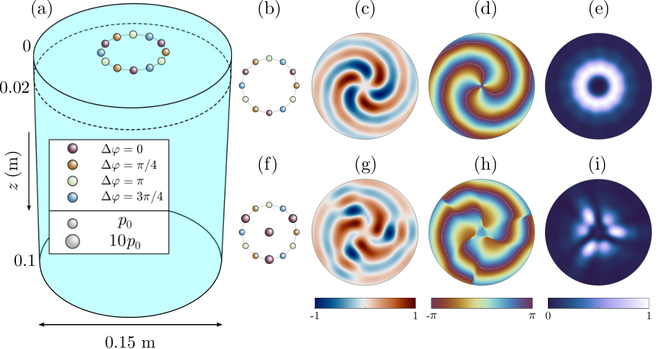
Conventional methods for exciting acoustic beams that carry orbital angular momentum rely on discrete phased sources, such as circular arrays of loudspeakers. The interference of the monopolar-like sources then approximates a beam with a helical phase-front. Often acoustic waveguides are used to enable the beam waist to be formed a desired distance away from the sources Gibson et al. 2018; Cromb et al. 2020. In Fig. 4 we show the discrete phased analogy via a frequency domain FEM simulation for two cases; (i) a ring of 12 phased point acoustic sources with equal amplitude, and (ii) the same ring but with additional central source and amplitude variation. We included this model purely as a qualitative analogue to the acoustic OAM mode excited by the pipe; the vector elastic system cannot be reduced to a purely scalar (monopole) source as higher order vector components (e.g. dipole) contribute Bruus 2012; Toftul et al. 2019. The geometry considered is such that the point sources lie on a ring of diameter , as if placed at the mid-point of the pipe thickness, lying atop a cylindrical volume of water deep and in diameter, akin to the FEM simulations of the main experiment (see see Appendix C). Each source is coloured to represent the relative phase shift (of radians) to the adjacent sources, and has an amplitude represented by their relative size. The array is chosen so that a topological charge of is achieved. Figures 4(c-d) show, for case (i), the real pressure field, phase, and acoustic intensity respectively for an excitation frequency of at a distance from the source plane. As there is no other sources present this well approximates an acoustic beam carrying OAM. For case (ii), an additional source is present at the centre of the ring, and the amplitude of three sources is also modified.
The eSPP considered throughout can be seen to act as a continuous phased acoustic source, with the phase profile determined by the circumferential order of the flexural mode, as shown in Fig. 3(a). The analogy to the additional source in case (ii) represents the amplitude modulation in the experiment due to the background provided by the unconverted compressional wave, and other modes present in the pipe. This intuitive analogy gives qualitative agreement to the experimental fields. As such we pose that the pipe acts as an amplitude-modulated-continuous-phased source for acoustic OAM beams.
conclusions and perspectives
Generating acoustic vortex beams that carry OAM has been instrumental to the development of optical and acoustic tweezers. Specifically in acoustics, the generation of these modes conventionally relies on discrete phased arrays. By considering the elastic orbital angular momentum associated with compressional motion we have demonstrated the first experimental observation of elastic orbital angular momentum transfer from guided flexural modes in a pipe to acoustic waves in a fluid, verifying the experiment proposed in Chaplain et al. 2022, and thus providing a new avenue to generate acoustic OAM beams.
The applications of this phenomena are therefore aligned with those of acoustic tweezers, including sensing, communication and microfluidic control. Extensions of this new methodology are anticipated to fluid-filled pipes, where there exist attractive applications in, for example, non-destructive testing in pipe-networks.
Acknowledgements
G.J.C gratefully acknowledges financial support from the Royal Commission for the Exhibition of 1851 in the form of a Research Fellowship. J.M.D.P acknowledges the financial support from the H2020 FET-proactive project MetaVEH under grant agreement No. 952039. T.A.S gratefully acknowledges financial support from DSTL. The authors thank Prof. R. V. Craster, Prof. A. P. Hibbins and Dr. S. A. R. Horsely for useful conversations, and to G. T. Starkey for assistance in mount construction.
Appendix A Experimental Setup
Measurements were performed in a water tank without wall or surface treatments, with dimensions m (). The pipe was suspended vertically above the tank using nylon fishing line attached to a mount so that the end of the pipe was submerged approximately into the fluid (Fig. 1(d)); the seal on the capped end of the pipe ensures fluid is present within the pipe, up to the same depth of submersion. A piezoelectric PZT-8 disc of thickness and diameter was glued to the centre of the cap to provide excitation with a 5-cycle pulse centred on . The piezoelectric excites the mode which then efficiently excites the mode via mode conversion in the spiral region as outlined in Chaplain and De Ponti 2022.
To obtain pressure field maps of sound radiated from the submerged end of the pipe, the signal at the detection hydrophone (Brüel & Kjær 8103 hydrophone) was scanned in space using an scanning stage (in-house built with Aerotech controllers). The hydrophone was vertically mounted to a perforated perspex arm, to match the propagation direction of the acoustic field. The acoustic propagation was then spatially mapped in steps across a area centred beneath the pipe; the voltage, , from the detector was recorded as a function of time, , at each position in the scan. At each spatial point, the acoustic pressure field is averaged over the detecting area of the hydrophone head and the signals were averaged in time over 20 repeat pulses to improve the signal-to-noise ratio. The detector was sampled with sample rate to record the signal for at each point. The resulting usable frequency range for this source-detector response function was between . The resulting signals are time-windowed corresponding to the time-of-flight of the flexural wave packet so that the pressure field excited by the pulse is isolated in the fluid. We then confirm this is a dominant mode of the system through Dynamic Mode Decomposition.
Appendix B Dynamic Mode Decomposition
Dynamic Mode Decomposition is a technique developed by Schmid Schmid 2010 that enables a data set, be it numerical or experimental, to be analysed so that the dominant dynamics can be observed. This is a particularly attractive method here given the large number of modes excited within the pipe. Here we briefly outline the methodology following Schmid 2010.
DMD rests on representing an original time-series data set as a sum of mode shapes associated with the radian frequency such that
| (9) |
where is the mode shape. The data we analyse is the temporal evolution of the acoustic pressure at a series of grid-points in space. The data is rearranged into a single matrix such that each column represents on frame of the data:
| (10) |
Where is the complete data set and is the data at times . As the governing equations for the acoustic propagation are linear, the data at each time step can be related by a matrix such that
| (11) |
and thus
| (12) |
The dynamics of the system are then governed by the eigenvalues and eigenvectors of , which can be approximated by several numerical methods. Here, as in Schmid’s original paper Schmid 2010, we use singular value decomposition (SVD). We shall also consider the shifted matrix
| (13) |
for sufficiently large (i.e. a long time signal) and will have a near identical structure. By SVD, we write
| (14) |
where and contain the left- and right-singular vectors respectively, with the singular values along the diagonal of . If the relative size of successive singular values to the first few is small, then the size of the matrices can be reduced, with the reduced forms subsequently written as e.g. . The matrix contains the so-called principal directions, that are used to rewrite the data in a new basis and define
| (15) |
Using the reduced forms, (13) then becomes
| (16) | ||||
This approximation of then contains all the information needed to take one frame of the data to the next. The eigenvalues and eigenvectors of then are obtained by converting back to the original basis such that
| (17) |
where is the mode for the eigenvector . The results of this decomposition on the time-series data obtained in the experiments is shown in Fig. 2(e-f), showing that this is a dominant mode shape.
Appendix C Finite Element Modelling
The commercial FEM software COMSOL Multiphysics® was used to perform time domain simulations of the suspended pipe geometry. The acoustics and structural mechanics module were used with acoustic-solid interaction to couple the displacement field in the pipe with the acoustic pressure fields in the air and water. A schematic of the simulation domain is shown in Fig. 5, with cylindrical wave radiation conditions on the dashed boundaries. The same 5-cycle tone burst, centred on excitation was used and applied as a boundary load to the top cap of the pipe (area marked with magenta circle in Fig. 5) to simulate the effect of the piezoelectic disc source (not actually modelled in the geometry). The numerical pressure field was then extracted in the fluid, with the same spatial resolution as used in the experiment. Fourier analysis was then performed via the Fast Fourier Transform to obtain the spatial-frequency spectra, as done in the experiment. The results were analysed at several planes beneath the pipe to determine the position of the acoustic centre of the hydrophone and used to show the excitation of a LG-like acoustic beam near the submerged surface of the pipe (Fig. 3).
For the comparison with a discrete phased acoustic array, only the acoustics module was used, with the simulation domain shown in Fig. 4, using monopolar-like point acoustic sources. The simulation domain here matches the region of water in the main simulation.

References
- Shen et al. (2019) Y. Shen, X. Wang, Z. Xie, C. Min, X. Fu, Q. Liu, M. Gong, and X. Yuan, Optical vortices 30 years on: Oam manipulation from topological charge to multiple singularities, Light: Science & Applications 8, 1 (2019).
- Allen et al. (1992) L. Allen, M. W. Beijersbergen, R. Spreeuw, and J. Woerdman, Orbital angular momentum of light and the transformation of Laguerre-Gaussian laser modes, Phys. Rev. A 45, 8185 (1992).
- Fontaine et al. (2019) N. K. Fontaine, R. Ryf, H. Chen, D. T. Neilson, K. Kim, and J. Carpenter, Laguerre-gaussian mode sorter, Nat. Comms. 10, 1 (2019).
- Yao and Padgett (2011) A. M. Yao and M. J. Padgett, Orbital angular momentum: origins, behavior and applications, Adv. Opt. Photonics 3, 161 (2011).
- Loke et al. (2014) V. L. Loke, T. Asavei, A. B. Stilgoe, T. A. Nieminen, and H. Rubinsztein-Dunlop, Driving corrugated donut rotors with laguerre-gauss beams, Opt. Express 22, 19692 (2014).
- Allen et al. (2016) L. Allen, S. M. Barnett, and M. J. Padgett, Optical angular momentum (CRC press, 2016).
- Padgett (2017) M. J. Padgett, Orbital angular momentum 25 years on, Opt. Express 25, 11265 (2017).
- Barnett et al. (2017) S. M. Barnett, M. Babiker, and M. J. Padgett, Optical orbital angular momentum, Philos. Trans. R. Soc. A 375, 20150444 (2017).
- Higgins (1992) T. V. Higgins, Spiral waveplate design produces radially polarized laser light, Laser Focus World 28, 18 (1992).
- Oemrawsingh et al. (2004) S. Oemrawsingh, J. Van Houwelingen, E. Eliel, J. Woerdman, E. Verstegen, J. Kloosterboer, et al., Production and characterization of spiral phase plates for optical wavelengths, Appl. Opt. 43, 688 (2004).
- O’Neil et al. (2002) A. O’Neil, I. MacVicar, L. Allen, and M. Padgett, Intrinsic and extrinsic nature of the orbital angular momentum of a light beam, Phys. Rev. Lett. 88, 053601 (2002).
- McGloin et al. (2003) D. McGloin, V. Garcés-Chávez, and K. Dholakia, Interfering bessel beams for optical micromanipulation, Opt. Lett. 28, 657 (2003).
- Vasilyeu et al. (2009) R. Vasilyeu, A. Dudley, N. Khilo, and A. Forbes, Generating superpositions of higher–order bessel beams, Opt. Express 17, 23389 (2009).
- Leach et al. (2004) J. Leach, M. R. Dennis, J. Courtial, and M. J. Padgett, Knotted threads of darkness, Nature 432, 165 (2004).
- Leach et al. (2005) J. Leach, M. R. Dennis, J. Courtial, and M. J. Padgett, Vortex knots in light, New J. Phys. 7, 55 (2005).
- Götte et al. (2008) J. B. Götte, K. O’Holleran, D. Preece, F. Flossmann, S. Franke-Arnold, S. M. Barnett, and M. J. Padgett, Light beams with fractional orbital angular momentum and their vortex structure, Opt. Express 16, 993 (2008).
- Morgan et al. (2017) K. Morgan, J. Miller, W. Li, Y. Li, and E. Johnson, Higher order bessel beams integrated in time (hobbit) for free space underwater sensing and communication, in OCEANS 2017-Anchorage (IEEE, 2017) pp. 1–4.
- Bliokh and Nori (2019) K. Y. Bliokh and F. Nori, Spin and orbital angular momenta of acoustic beams, Phys. Rev. B 99, 174310 (2019).
- Zhang and Marston (2011) L. Zhang and P. L. Marston, Angular momentum flux of nonparaxial acoustic vortex beams and torques on axisymmetric objects, Phys. Rev. E 84, 065601 (2011).
- Zhang (2018) L. Zhang, Reversals of orbital angular momentum transfer and radiation torque, Phys. Rev. Appl. 10, 034039 (2018).
- Hong et al. (2015) Z. Hong, J. Zhang, and B. W. Drinkwater, Observation of orbital angular momentum transfer from bessel-shaped acoustic vortices to diphasic liquid-microparticle mixtures, Physical review letters 114, 214301 (2015).
- Baresch et al. (2016) D. Baresch, J.-L. Thomas, and R. Marchiano, Observation of a single-beam gradient force acoustical trap for elastic particles: acoustical tweezers, Physical review letters 116, 024301 (2016).
- Shi et al. (2017) C. Shi, M. Dubois, Y. Wang, and X. Zhang, High-speed acoustic communication by multiplexing orbital angular momentum, Proc. Natl. Acad. Sci. 114, 7250 (2017).
- Marzo et al. (2018) A. Marzo, M. Caleap, and B. W. Drinkwater, Acoustic virtual vortices with tunable orbital angular momentum for trapping of mie particles, Physical review letters 120, 044301 (2018).
- Hefner and Marston (1998) B. T. Hefner and P. L. Marston, Acoustical helicoidal waves and laguerre-gaussian beams: Applications to scattering and to angular momentum transport, J. Acoust. Soc. Am. 103, 2971 (1998).
- Hefner and Marston (1999) B. T. Hefner and P. L. Marston, An acoustical helicoidal wave transducer with applications for the alignment of ultrasonic and underwater systems, J. Acoust. Soc. Am. 106, 3313 (1999).
- Jiang et al. (2016) X. Jiang, Y. Li, B. Liang, J.-c. Cheng, and L. Zhang, Convert acoustic resonances to orbital angular momentum, Phys. Rev. Lett. 117, 034301 (2016).
- Naify et al. (2016) C. J. Naify, C. A. Rohde, T. P. Martin, M. Nicholas, M. D. Guild, and G. J. Orris, Generation of topologically diverse acoustic vortex beams using a compact metamaterial aperture, Appl. Phys. Lett. 108, 223503 (2016).
- Guo et al. (2019) Z. Guo, H. Liu, H. Zhou, K. Zhou, S. Wang, F. Shen, Y. Gong, J. Gao, S. Liu, and K. Guo, High-order acoustic vortex field generation based on a metasurface, Phys. Rev. E 100, 053315 (2019).
- Gibson et al. (2018) G. M. Gibson, E. Toninelli, S. A. Horsley, G. C. Spalding, E. Hendry, D. B. Phillips, and M. J. Padgett, Reversal of orbital angular momentum arising from an extreme doppler shift, Proc. Natl. Acad. Sci. 115, 3800 (2018).
- Antonacci et al. (2019) G. Antonacci, D. Caprini, and G. Ruocco, Demonstration of self-healing and scattering resilience of acoustic bessel beams, Appl. Phys. Lett. 114, 013502 (2019).
- Cromb et al. (2020) M. Cromb, G. M. Gibson, E. Toninelli, M. J. Padgett, E. M. Wright, and D. Faccio, Amplification of waves from a rotating body, Nat. Phys. 16, 1069 (2020).
- Marchiano and Thomas (2005) R. Marchiano and J.-L. Thomas, Synthesis and analysis of linear and nonlinear acoustical vortices, Phys. Rev. E 71, 066616 (2005).
- Basistiy et al. (1993) I. Basistiy, V. Y. Bazhenov, M. Soskin, and M. V. Vasnetsov, Optics of light beams with screw dislocations, Opt. Commum. 103, 422 (1993).
- Zambrini and Barnett (2006) R. Zambrini and S. M. Barnett, Quasi-intrinsic angular momentum and the measurement of its spectrum, Phys. Rev. Lett. 96, 113901 (2006).
- Nakane and Kohno (2018) J. J. Nakane and H. Kohno, Angular momentum of phonons and its application to single-spin relaxation, Physical Review B 97, 174403 (2018).
- Long et al. (2018) Y. Long, J. Ren, and H. Chen, Intrinsic spin of elastic waves, Proc. Natl. Acad. Sci. 115, 9951 (2018).
- Chaplain et al. (2022) G. J. Chaplain, J. M. De Ponti, and R. V. Craster, Elastic orbital angular momentum, Phys. Rev. Lett. 128, 064301 (2022).
- Bliokh (2022) K. Y. Bliokh, Elastic spin and orbital angular momenta, arXiv preprint arXiv:2204.13037 (2022).
- Durnin et al. (1987) J. Durnin, J. Miceli Jr, and J. H. Eberly, Diffraction-free beams, Phys. Rev. Lett. 58, 1499 (1987).
- Landau and Lifshitz (1959) L. D. Landau and E. M. Lifshitz, Course of Theoretical Physics Vol 7: Theory and Elasticity (Pergamon press, 1959).
- Gazis (1959a) D. C. Gazis, Three-dimensional investigation of the propagation of waves in hollow circular cylinders. I. Analytical foundation, J. Acoust. Soc. Am. 31, 568 (1959a).
- Morand and Ohayon (1995) H. J. P. Morand and R. Ohayon, Fluid Structure Interaction (John Wiley & Sons, Chichester, 1995).
- Bermúdez et al. (2008) A. Bermúdez, P. Gamallo, L. Hervella-Nieto, R. Rodríguez, and D. Santamarina, Fluid–structure acoustic interaction, in Computational Acoustics of Noise Propagation in Fluids-Finite and Boundary Element Methods (Springer, 2008) pp. 253–286.
- COMSOL (2021) COMSOL, Solid Mechanics Module User’s Guide (Stockholm, Sweden, 2021).
- Franke-Arnold et al. (2008) S. Franke-Arnold, L. Allen, and M. Padgett, Advances in optical angular momentum, Laser & Photonics Reviews 2, 299 (2008).
- Chaplain and De Ponti (2022) G. Chaplain and J. De Ponti, The elastic spiral phase pipe, J. Sound Vib. 523, 116718 (2022).
- Gazis (1959b) D. C. Gazis, Three-dimensional investigation of the propagation of waves in hollow circular cylinders. II. Numerical results, J. Acoust. Soc. Am. 31, 573 (1959b).
- Silk and Bainton (1979) M. Silk and K. Bainton, The propagation in metal tubing of ultrasonic wave modes equivalent to Lamb waves, Ultrasonics 17, 11 (1979).
- Alleyne et al. (1998) D. N. Alleyne, M. J. S. Lowe, and P. Cawley, The Reflection of Guided Waves From Circumferential Notches in Pipes, J. Appl. Mech. 65, 635 (1998).
- Lowe et al. (1998) M. J. S. Lowe, D. N. Alleyne, and P. Cawley, The Mode Conversion of a Guided Wave by a Part-Circumferential Notch in a Pipe, J. Appl. Mech. 65, 649 (1998).
- Shin and Rose (1999) H. J. Shin and J. L. Rose, Guided waves by axisymmetric and non-axisymmetric surface loading on hollow cylinders, Ultrasonics 37, 355 (1999).
- Tang and Wu (2017) L. Tang and B. Wu, Excitation mechanism of flexural-guided wave modes F(1, 2) and F(1, 3) in pipes, J. Nondestruct. Eval. 36, 1 (2017).
- Lowe (2001) M. Lowe, Wave propagation — guided waves in structures, in Encyclopedia of Vibration, edited by S. Braun (Elsevier, Oxford, 2001) pp. 1551–1559.
- Kwun et al. (2008) H. Kwun, S. Y. Kim, H. Matsumoto, and S. Vinogradov, Detection of axial cracks in tube and pipe using torsional guided waves, in AIP Conference Proceedings, Vol. 975 (American Institute of Physics, 2008) pp. 193–199.
- Ratassepp et al. (2010) M. Ratassepp, S. Fletcher, and M. Lowe, Scattering of the fundamental torsional mode at an axial crack in a pipe, J. Acoust. Soc. Am. 127, 730 (2010).
- Beijersbergen et al. (1994) M. Beijersbergen, R. Coerwinkel, M. Kristensen, and J. Woerdman, Helical-wavefront laser beams produced with a spiral phaseplate, Opt. Commum. 112, 321 (1994).
- Adamou and Craster (2004) A. Adamou and R. Craster, Spectral methods for modelling guided waves in elastic media, J. Acoust. Soc. Am. 116, 1524 (2004).
- Ricci et al. (2012) F. Ricci, W. Löffler, and M. Van Exter, Instability of higher-order optical vortices analyzed with a multi-pinhole interferometer, Opt. Express 20, 22961 (2012).
- Berry and Dennis (2001) M. V. Berry and M. R. Dennis, Knotted and linked phase singularities in monochromatic waves, Proc. R. Soc. A 457, 2251 (2001).
- Schmid (2010) P. J. Schmid, Dynamic mode decomposition of numerical and experimental data, J. Fluid Mech. 656, 5–28 (2010).
- Bruus (2012) H. Bruus, Acoustofluidics 7: The acoustic radiation force on small particles, Lab on a Chip 12, 1014 (2012).
- Toftul et al. (2019) I. Toftul, K. Bliokh, M. I. Petrov, and F. Nori, Acoustic radiation force and torque on small particles as measures of the canonical momentum and spin densities, Phys. Rev. Lett. 123, 183901 (2019).