Clustering units in neural networks: upstream vs downstream information
Abstract
It has been hypothesized that some form of “modular” structure in artificial neural networks should be useful for learning, compositionality, and generalization. However, defining and quantifying modularity remains an open problem. We cast the problem of detecting functional modules into the problem of detecting clusters of similar-functioning units. This begs the question of what makes two units functionally similar. For this, we consider two broad families of methods: those that define similarity based on how units respond to structured variations in inputs (“upstream”), and those based on how variations in hidden unit activations affect outputs (“downstream”). We conduct an empirical study quantifying modularity of hidden layer representations of simple feedforward, fully connected networks, across a range of hyperparameters. For each model, we quantify pairwise associations between hidden units in each layer using a variety of both upstream and downstream measures, then cluster them by maximizing their “modularity score” using established tools from network science. We find two surprising results: first, dropout dramatically increased modularity, while other forms of weight regularization had more modest effects. Second, although we observe that there is usually good agreement about clusters within both upstream methods and downstream methods, there is little agreement about the cluster assignments across these two families of methods. This has important implications for representation-learning, as it suggests that finding modular representations that reflect structure in inputs (e.g. disentanglement) may be a distinct goal from learning modular representations that reflect structure in outputs (e.g. compositionality).
1 Introduction

Modularity is a design principle in which systems that solve complex problems are decomposed into sub-systems that solve simpler problems and that can be independently analyzed, debugged, and recombined for new tasks. From an engineering perspective, modular design has many benefits, such as increased robustness and fast adaptation to new problems (Simon 1962). It is well-known that learning systems benefit from structure adapted to the problem at hand (Denker et al. 1987), and many real-world problems indeed can be decomposed into sub-problems. It is no surprise, then, that modularity is considered a normative design principle of evolved biological systems (Wagner et al. 2007; Lipson 2007), including in biological neural networks (Azam 2000; Kashtan & Alon 2005; Kashtan et al. 2007; Clune et al. 2013), and one from which artificial neural networks (ANNs) can benefit.
Despite these strong intuitions, formally defining and quantifying the modularity of a given system remains an open problem (cf. Simon 1962; Lipson 2007). It is generally accepted that, by definition, modular systems decompose into sub-systems that implement functions that solve sub-problems. Characterizing modules in ANNs therefore begs the question: when are two parts of a network involved in the same “function” (Csordás et al. 2021)? In this paper, we ask this question at the level of pairs of hidden units. That is, we consider a variety of methods for measuring the “functional similarity” of any given pair of hidden units, and we operationalize a “module” as a cluster of similarly-functioning units (Figure 1A-B). This definition is not intended to solve the question of what a module is, but to provide a tractable basis for experimenting with various ideas related to modularity, such as how it is affected by regularization.
One goal of this paper is simply to raise awareness of qualitative differences between “upstream” and “downstream” ways of thinking about neural representations and the functions they are involved in (Figure 1C). In section 3, we make these definitions quantitative and give details for our method for detecting and quantifying functional modules in the hidden layers of trained neural networks by clustering units into similarly-functioning groups. This framework allows us to directly compare a variety of proxies for the amount of modularity a network exhibits. Experimental results are described in section 4. In addition to quantitatively scoring modularity, we further investigate whether different similarity measures agree on which units belong to which module. Surprisingly, we find that modules discovered according to “upstream” measures of functional similarity are consistently distinct from those discovered using “downstream” measures. Although we do not consider regularization methods explicitly designed to produce modular designs, these initial empirical results nonetheless call for a deeper look at how the “function” of a representation is defined, as well as why and in which situations modules may be useful.
2 Related Work
The study of modularity in neural networks has a long history (Clune et al. 2013; Amer & Maul 2019). One common source of inspiration from biology is the functional dissociation of “what” and “where” pathways in the ventral and dorsal streams of the brain, respectively (Goodale & Milner 1992). Each of these pathways can be seen as a specialized module (and may be further decomposed into submodules), and many previous experiments on modularity in artificial neural networks have explored principles that would result in similarly distinct what/where information processing in ANNs (Rueckl et al. 1989; Jacobs et al. 1991; Di Ferdinando et al. 2001; Bakhtiari et al. 2021). A key difference to this line of work is that, rather than specifying the functional role of modules ahead of time, such as one module being “what” and another being “where,” our work seeks to identify distinct functional clusters in trained networks.
Broadly speaking, there are two families of approaches to modularity in neural networks, corresponding to different ways of thinking about the function of parts of a network. The structural modularity family of approaches defines function in terms of network weights and how sub-networks connect to other sub-networks, and so modules are defined as densely intra- and sparsely inter-connected sub-networks (Watanabe et al. 2018; Amer & Maul 2019; Csordás et al. 2021; Filan et al. 2021). The functional modularity family of approaches emphasizes network activations rather than weights, or the information represented by those activations. These include disentanglement, compositionality, invariance, and others(Bengio et al. 2013; Higgins et al. 2018; Andreas 2019; Scholkopf et al. 2021). The relationship between structural and functional modules is not clear – while it certainly seems that they are (or ought to be) correlated (Lipson 2007), it has been observed empirically that even extremely sparse inter-module-connectivity does not always guarantee functional separation of information-processing (Béna & Goodman 2021). In this work, we take the functional approach, based on the assumption that structural modularity is itself only useful insofar as it supports distinct functions of the units, and that often distinct functions must share information, making strict structural delineations potentially counterproductive. For example, knowing “what” an object is in a challenging visual scene helps localize “where” it is, and vice versa.
Our work is perhaps most closely related to a series of papers by Watanabe and colleagues (Watanabe et al. 2018; Watanabe 2019; Watanabe et al. 2019; Watanabe et al. 2020) in which trained networks are decomposed into clusters of “similar” units with the aim of understanding and simplifying those networks. They quantify the similarity of units using a combination of both incoming and outgoing weights. This is similar in spirit to our goal of identifying modules by clustering units, but an interesting contrast to our approach, where we find stark differences between “upstream” and “downstream” similarity.
3 Quantifying modularity by clustering similarity
We split the problem of identifying functional modules into two stages (Figure 1D): scoring the pairwise similarity of units, then clustering based on similarity. To simplify, we only apply these steps separately to each hidden layer, but in principle modules could be scored in the same way after concatenating layers together. Section 3.1 below defines the set of pairwise functional similarity methods we use, and Section 3.2 describes the clustering stage.
While we focus on similarity between pairs of individual units, our approach is related to, and inspired by, the question of what makes neural representations “similar” when comparing entire populations of neurons to each other (Kornblith et al. 2019). Rather than finding clusters-of-similar-neurons as we do here, one could instead define modules in terms of dissimilarity-between-clusters-of-neurons. In preliminary work, we explored such a definition of functional modules, using representational (dis)similarity between sub-populations of neurons. The main challenge of this approach is that existing representational-similarity methods are highly sensitive to dimensionality (the number of neurons in each cluster), and it is not obvious how best to control for this when computing dissimilarity between clusters such that the method is not biased to prefer large or small cluster sizes.11 1 Note that dimensionality is not a problem for other applications of representational (dis)similarity methods, since the population size is traditionally fixed in any single analysis. To further motivate our method, note that representational similarity analysis is closely related to tests for statistical (in)dependence between populations of neurons (Kornblith et al. 2019; Gretton et al. 2005; Cortes et al. 2012), and so the problem of finding mutually “dissimilar” modules is analogous to the problem of finding independent subspaces (Hyvärinen et al. 2001; Gutch & Theis 2007). In Independent Subspace Analysis (ISA), there is an analogous problem of determining what constitutes a surprising amount of dependence between subspaces of different dimensions, and various methods have been proposed with different inductive biases (Wu et al. 2021; Bach & Jordan 2004; Bach & Jordan 2003; Póczos & Lõrincz 2005). However, Palmer & Makeig 2012 showed that a solution to the problem of detecting independent subspaces is to simply cluster the individual dimensions of the space. This provides some justification for the methods we use here: some technicalities22 2 First, one can construct pathological examples of dependent subspaces but where all individual variables are independent, so pairwise independence between all elements in a cluster cannot guarantee independent clusters. Second, summing or averaging pairwise dissimilarity across clusters will give quantitatively different value than measuring dissimilarity between the populations, but this brings us back to the dimensionality problem already discussed. notwithstanding, the problem of finding subspaces of neural activity with “dissimilar” representations is, in many cases, reducible to the problem of clustering individual units based on pairwise similarity, as we do here.
3.1 Quantifying pairwise similarity of hidden units
What makes two hidden units “functionally similar”? In other words, we seek some similarity function that takes as input a neural network evaluated on a dataset to solve task and produces an matrix of non-negative similarity scores for all pairs among the hidden units. We further require that the resulting matrix is symmetric, or . Importantly, allowing to depend on the task opens the door to similarity measures where units are considered similar based on their downstream contribution to a particular loss function.
Similarity by covariance.
The first similarity measure we consider is the absolute value covariance of hidden unit activities across inputs. Let be the th input in the dataset, and be the response of the th hidden unit to input , with . Then, we define similarity as
| (1) |
where is the number of items in and is the mean response of unit on the given dataset. Intuitively, the absolute value covariance quantifies the statistical dependence of two units across inputs, making it an upstream measure of similarity. corresponds to some classic notions of “disentanglement”: to the extent that the rows and columns of can be sorted to have highly block-diagonal structure, this means that hidden units cluster into statistically independent – or at least uncorrelated – groups. This is also similar in spirit to Representational Similarity Analysis, where the similarity of sets of units is quantified using some (often kernel-based) measure of their independence on a given dataset (Kornblith et al. 2019).33 3 In pathological cases, it is possible for random variables to be pairwise-independent but groupwise-dependent, which could be considered a limitation of our method. On the other hand, it is not at all clear how one could use groupwise-independence for modularity detection, since there are nontrivial interactions between group dimensionality, the marginal distributions of neural activity, and choice of kernel. We leave this for future work.
Similarity by input sensitivity.
While quantifies similarity of responses across inputs, we next consider a measure of similar sensitivity to single inputs, which is then averaged over . Let denote the Jacobian matrix of partial derivatives of each hidden unit with respect to each of the input dimensions. Then, we say two units and are similarly sensitive to input changes on input if the dot product between the th and th row of has high absolute-value magnitude. In matrix notation over the entire dataset, we use
| (2) |
where the superscript “i-sens” should be read as the “input sensitivity.”
Similarity by last-layer sensitivity.
Let denote the last-layer activity of the network. Using the same Jacobian notation as above, let denote the matrix of partial derivatives of the last layer with respect to changes in the hidden activities . Then, we define similarity by output sensitivity as
| (3) |
likewise with “o-sens” to be read as “output-sensitivity.” Note that both and depend on the particular input , but this has been left implicit in the notation to reduce clutter.
Similarity by the loss Hessian.
The “function” of a hidden unit might usefully be thought of in terms of its contribution to the task or tasks it was trained on. To quote Lipson 2007,
“In order to measure modularity, one must have a quantitative definition of function… It is then possible to take an arbitrary chunk of a system and measure the dependency of the system function on elements within that chunk. The more that the dependency itself depends on elements outside the chunk, the less the function of that chunk is localized, and hence the less modular it is.” (Lipson 2007).
Lipson then goes on to suggest that the “dependence of system function on elements” can be expressed as a derivative or gradient, and that the dependence of that dependence on other parts of the system can be expressed as the second derivative or Hessian. Towards this conception of modular functions on a particular task, we use the following definition of similarity:
| (4) |
where is the scalar loss function for the task, and should be understood to depend on the particular input . Importantly, each Hessian on the right hand side is taken with respect to the activity of hidden units, not with respect to the network parameters as it is typically defined.
To summarize, equations (1) through (4) provide four different methods to quantify pairwise similarity of hidden units. and are upstream, while and are downstream. All four take values in , however, it is not clear if the raw magnitudes matter, or only relative (normalized) magnitudes. Take for instance. Kornblith et al. 2019 argue that hidden-unit covariance is more meaningful than correlation, since the principal directions of variation both affect learning and have been shown to correlate with meaningful perceptual differences for human observers. On the other hand, we do not want our measure of modularity, which is a global property of an entire layer, to be skewed by a small number of highly variable units. Further, the community-detection algorithm we use for clustering below has been primarily developed and tested on unweighted and undirected graphs. For these reasons, we introduce an optional normalized version of each of the above four un-normalized similarity measures:
| (5) |
where is a small positive value included for numerical stability. Whereas , the normalized values are restricted to . In total, this gives us eight methods to quantify pairwise similarity. These can be thought of as 2x2x2 product of methods, as shown in the color scheme in Figure 2: the upstream vs downstream axis, the unnormalized vs normalized axis, and the covariance vs gradient (i.e. sensitivity) axis. We group together both and under the term “covariance” because the Hessian is closely related to the covariance of gradient vectors of the loss across inputs.
3.2 Quantifying modularity by clustering
Decomposing a set into clusters that are maximally similar within clusters and maximally dissimilar across clusters is a well-studied problem in graph theory and network science. In particular, Girvan & Newman 2002 proposed a method that cuts a graph into its maximally modular subgraphs (Girvan & Newman 2002; Newman & Girvan 2004; Newman 2006), and this tool has previously been used to study modular neural networks (Amer & Maul 2019; Béna & Goodman 2021).
We apply this tool from graph theory to our problem of detecting functional modules in neural networks by constructing an adjacency matrix from the similarity matrix by simply removing the diagonal (self-similarity):
Given , we can simplify later notation by first constructing the normalized adjacency matrix, , whose elements all sum to one:
or, more compactly, where is a column vector of length containing all ones. Let be an matrix that represents cluster assignments for each of units to a maximum of different clusters. Cluster assignments can be “hard” () or “soft” (), but in either case the constraint must be met, i.e. that the sum of cluster assignments for each unit is .44 4 While we only consider hard cluster assignments in our experiments below, we have encountered cases where is maximized by soft cluster assignments, so we include it in the definition here for completeness. If an entire column of is zero, that cluster is unused, so only provides an upper-limit to the number of clusters, and in practice we set . Girvan & Newman 2002 propose the following score to quantify the level of “modularity” when partitioning the normalized adjacency matrix into the cluster assignments :
| (6) |
The first term sums the total connectivity (or, in our case, similarity) of units that share a cluster. By itself, this term is maximized when assigns all units to a single cluster. The second term gives the expected connectivity within each cluster under a null model where the elements of are interpreted as the joint probability of a connection, and so is the product of marginal probabilities of each unit’s connections. This second term encourages to place units into the same cluster only if they are more similar to each other than “chance.” Together, equation (6) is maximized by partitioning into clusters that are strongly intra-connected and weakly inter-connected.
We define the modularity of a set of neural network units as the maximum achievable over all :
| (7) |
To summarize, to divide a given pairwise similarity matrix into modules, we first construct from , then we find the cluster assignments that give the maximal value . Importantly, this optimization process provides two pieces of information: a modularity score which quantifies the amount of modularity in a set of neurons, for a given similarity measure. We also get the actual cluster assignments , which provide additional information and can be compared across different similarity measures. Given a set of cluster assignments , we quantify the number of clusters by first getting the fraction of units in each cluster, . We then use the formula for discrete entropy to measure the dispersion of cluster sizes: . Finally we say that the number of clusters in is
| (8) |
We emphasize that discovering the number of clusters in is included automatically in the optimization process; we set the maximum number of clusters equal to the number of hidden units , but in our experiments we find that rarely uses more than 6 clusters for hidden layers with 64 units (Supplemental Figure S4).
It is important to recognize that the sense of the word “modularity” in graph theory is in some important ways distinct from its meaning in terms of engineering functionally modular systems. In graph-theoretic terms, a “module” is a cluster of nodes that are highly intra-connected and weakly inter-connected to other parts of the network, defined formally by (Girvan & Newman 2002; Newman & Girvan 2004). This definition of graph modularity uses a particular idea of a “null model” based on random connectivity between nodes in a graph (Amer & Maul 2019). While this null-model of graph connectivity enjoys a good deal of historical precedence in the theory of randomly-connected graphs, where unweighted graphs are commonly studied in terms of the probability of connection between random pairs of nodes, it is not obvious that the same sort of null model applies to groups of “functionally similar” units in an ANN. This relates to the earlier discussion of ISA, and provides a possibly unsatisfying answer to the question of what counts as a “surprising” amount of statistical independence between clusters; using makes the implicit choice that the product of average pairwise similarity, , gives the “expected” similarity between units. An important problem for future work will be to closely reexamine the question of what makes neural populations functionally similar or dissimilar, above and beyond statistical similarity (Csordás et al. 2021; Kornblith et al. 2019), and what constitutes a surprising amount of (dis)similarity that may be indicative of modular design.
Finding exactly is NP-complete (Brandes et al. 2008), so in practice we use a variation on the approximate method proposed by (Newman 2006). Briefly, the approximation works in two steps: first, an initial set of cluster assignments is constructed using a fast spectral initialization method that, similar to other spectral clustering algorithms, recursively divides units into clusters based on the sign of eigenvectors of the matrix and its submatrices. Only subdivisions that increase are kept. In the second step, we use a Monte Carlo method that repeatedly selects a random unit then resamples its cluster assignment, holding the other assignments fixed. This resampling step involves a kind of exploration/exploitation trade-off: may decrease slightly on each move to potentially find a better global optimum. We found that it was beneficial to control the entropy of each step using a temperature parameter, to ensure that a good explore/exploit balance was struck for all . Supplemental Figure S2 shows that both the initialization and the Monte Carlo steps play a crucial role in finding , consistent with the observations of (Newman 2006). Full algorithms are given in Appendix A.1.
4 Experiments
4.1 Setup and initial hypotheses
| L2 (weight decay) | L1 weight penalty | dropout prob. |
|---|---|---|
| logspace(-5,-1,9) | 0.0 | 0.0 |
| 1e-5 | logspace(-5,-2,7) | 0.0 |
| 1e-5 | 0.0 | linspace(0.05,0.7,14) |
Because our primary goal is to understand the behavior of the various notions of modularity above, i.e. based on the eight different methods for quantifying pairwise similarity introduced in the previous section, we opted to study a large collection of simple networks trained on MNIST (LeCun et al. 1998). All pairwise similarity scores were computed using held-out test data. We trained 270 models, comprising 9 runs of each of 30 regularization settings, summarized in Table 1. We defined (input layer) as the raw dimensional pixel inputs and (output layer) as the dimensional class logits. We used the same basic feedforward architecture for all models, comprising two layers of hidden activity connected by three layers of fully-connected weights: Linear(784, 64), ReLU, dropout(p), Linear(64, 64), ReLU, dropout(p), Linear(64, 10). We analyzed modularity in the two dimensional hidden layers following the dropout operations. We discarded 21 models that achieved less than 80% test accuracy for a total of 249 trained models (this only happened at extremely high regularization). Summary statistics of model behavior as a function of regularization strength are shown in Supplementary Figure S1. For reference values, we also performed all analyses on 500 randomly initialized models with zero training. Models were written and trained using PyTorch (Paszke et al. 2019) and PyTorch Lightning55 5 https://www.pytorchlightning.ai/, and all compute jobs were run on a private server and managed using GNU Parallel (Tange 2011). Code is publicly available at https://github.com/wrongu/modularity.
Before running these experiments, we hypothesized that
- 1.
Dropout would decrease modularity by encouraging functions to be “spread out” over many units.
- 2.
L2 regularization (weight decay) would minimally impact modularity, since the L2 norm is invariant to rotation while modularity depends on axis-alignment.
- 3.
L1 regularization on weights would increase modularity by encouraging sparsity between subnetworks.
- 4.
All similarity measures would be qualitatively consistent with each other.
As shown below, all four of these hypotheses turned out to be wrong, to varying degrees.
4.2 How modularity depends on regularization
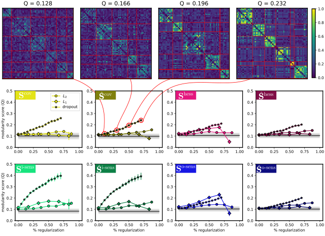
Figure 3 shows the dependence of trained networks’ modularity score () as a function of regularization strength for each of three types of regularization: an L2 penalty on the weights (weight decay), an L1 penalty on the weights, and dropout. The top row of Figure 3 shows four example matrices sorted by cluster, to help give an intuition behind the quantitative values of . In these examples, the increasing value of is driven by an increasing contrast between intra-cluster similarity and inter-cluster similarity. In this example, it also appears that the number and size of clusters remains roughly constant; this observation is confirmed by plotting the number of clusters versus regularization strength in Supplemental Figure S4.
Figure 3 shows a number of surprising patterns that contradict our initial predictions. First, and most saliently, we had predicted that dropout would reduce modularity, but found instead that it has the greatest effect on among the three regularization methods we tried. This is especially apparent in the upstream methods (first two columns of the figure), and is also stronger for the first hidden layer than the second (Supplemental Figure S3). In general, can increase either if the network partitions into a greater number of clusters, or if the contrast between clusters is exaggerated. We found that this dramatic effect of dropout on was accompanied by only minor changes to the number of clusters (Supplemental Figure S4), and so we can conclude that dropout increases by increasing the redundancy of hidden units. In other words, hidden units become more clusterable because they are driven towards behaving like functional replicas of each other, separately for each cluster. This observation echoes, and may explain, why dropout also increases the “clusterability” of network weights in a separate study (Filan et al. 2021).
The second surprising result in Figure 3 is that L2 regularization on the weights did, in fact, increase , whereas we had expected it to have no impact. Third, L1 regularization had a surprisingly weak effect, although its similarity to the L2 regularization results may be explained by the fact that they actually resulted in fairly commensurate sparsity in the trained weights (Supplemental Figure S1 bottom row). Fourth, we had expected few differences between the eight different methods for computing similarity, but there appear to be distinctive trends by similarity type both in Figure S3 as well as in the number of clusters detected (Supplemental Figure S4). The next section explores the question of similarity in the results in more detail.
4.3 Comparing modules discovered by different similarity methods
The previous section discussed idiosyncratic trends in the modularity scores as a function of both regularization strength and how pairwise similarity between units () is computed. However, such differences in the quantitative value of are difficult to interpret, and would largely be moot if the various methods agreed on the question of which units belong in which cluster. We now turn to the question of how similar the cluster assignments are across our eight definitions of functional modules. To minimize ambiguity, we will use the term “functional-similarity” to refer to , and “cluster-similarity” to refer to the comparison of different cluster assignments .

Quantifying similarity between cluster assignments is a well-studied problem, and we tested a variety of methods in the clusim Python package (Correia et al. 2018). All cluster-similarity methods we investigated gave qualitatively similar results, so here we report only the “Element Similarity” method of Gates et al. 2019, which is a value between 0 and 1 that is small when two cluster assignments are unrelated, and large when one cluster assignment is highly predictive of the other. Note that this cluster-similarity analysis is applied only to cluster assignments computed in the same layer of the same model. Thus, any dissimilarity in clusters that we see is due entirely to the different choices for functional-similarity, .
Figure 4a summarizes the results of this cluster-similarity analysis: there is a striking difference between clusters of units identified by “upstream” functional-similarity methods (, , , ) compared to “downstream” functional-similarity methods (, , , ). This analysis also reveals secondary structure within each class of upstream and downstream methods, where the choice to normalize not ( vs ) appears to matter little, and where there is a moderate difference between moment-based methods (, ) and gradient-based methods (, ). It is worth noting that some of this secondary structure is not robust across all types and levels of regularization; in particular, increasing L2 or L1 regularization strength appears to lead to (i) stronger dependence on normalization in the downstream methods, and (ii) a stronger overall agreement among the upstream methods (Supplemental Figure S5).
We next asked to what extent these cluster-similarity results are driven by training. As shown in Figure 4b, much of the structure in the downstream methods is unaffected by training (i.e. it is present in untrained models as well), while the cluster-similarity among different upstream methods only emerged as a result of training. Interestingly, this analysis further shows that the main upstream-vs-downstream distinction seen in Figure 4a is, in fact, attenuated slightly by training.
5 Conclusions
An abundance of “modular” designs in engineered and evolved systems has led many to speculate about the usefulness of modularity as a design principle (Lipson 2007), and how modular designs might be discovered by learning agents such as artificial neural networks (Amer & Maul 2019). Yet, precisely defining what a “module” is in a neural network is an open problem. Here we operationalized modules in a neural network as clusters of hidden units that perform similar functions, which leads naturally to the related question of what makes any given pair of units functionally similar? We introduced eight functional-similarity measures intended to cover a variety of intuitions about what makes two units similar, and empirically evaluated cluster-assignments based on each of these eight methods in a large number of trained models.
One surprising observation was that dropout increases modularity (as defined by ) (Filan et al. 2021), although this has little to do with the common-sense definition of a “module.” Instead, it is the byproduct of dropout causing subsets of units to behave like near-copies of each other, perhaps so that if one unit is dropped out, a copy of it provides similar information to the subsequent layer. To our knowledge, this redundancy-inducing effect of dropout has not been noted in the literature previously.
Our main result is that there is a crucial difference between defining “function” in terms of how units are driven by upstream inputs, and how units drive downstream outputs. While we studied this distinction between upstream and downstream similarity in the context of modularity and clustering, it speaks to the deeper and more general problem of how best to interpret neural representations. For example, some sub-disciplines of representation-learning (e.g. “disentanglement”) have long emphasized that a “good” neural representation is one where distinct features of the world drive distinct sub-populations or sub-spaces of neural activity (Higgins et al. 2018; Eastwood & Williams 2018; Ridgeway & Mozer 2018). This is an upstream way of thinking about what is represented, since it depends only on the relationship between inputs and the unit activations and does not take into account what happens downstream. Meanwhile, many have argued that the defining characteristic of a neural representation is its causal role in downstream behavior (Garson & Papineau 2019); this is, of course, a downstream way of thinking. At a high level, one way to interpret our results is is that upstream and downstream ways of thinking about neural representations are not necessarily aligned, even in trained networks. This observation is reminiscent of recent empirical work finding that “disentangled” representations in auto-encoders (an upstream concept) do not necessarily lead to improved performance or generalization to novel tasks (a downstream concept) (Locatello et al. 2019; Montero et al. 2021).
Despite its theoretical motivations, this is an empirical study. We trained over 250 feedforward, fully-connected neural networks on MNIST. While it is not obvious whether MNIST admits a meaningful “modular” solution, we expect that the main results we show here are likely robust, in particular (i) the effect of weight decay, an L1 weight penalty, and dropout, and (ii) misalignment between upstream and downstream definitions of neural similarity.
Our work raises the important questions: are neural representations defined by their inputs or their outputs? And, in what contexts is it beneficial for these to be aligned? We look forward to future work applying our methods to larger networks trained on more structured data, as well as recurrent networks. We also believe it will be valuable to evaluate the effect of attempting to maximize modularity, as we have defined it, during training, to see to what extent this is possible and whether it leads to performance benefits. Note that maximizing during training is challenging because (i) computing may require large batches, and more importantly (ii) optimizing is highly prone to local minima, since neural activity and cluster assignments will tend to reinforce each other, entrenching accidental clusters that appear at the beginning of training. We suspect that maintaining uncertainty over cluster assignments (e.g. using soft rather than hard cluster assignments) will be crucial if optimizing any of our proposed modularity metrics during training.
References
- Amer & Maul (2019) Mohammed Amer and Tomás Maul. A review of modularization techniques in artificial neural networks. Artificial Intelligence Review, 52(1):527–561, 2019. ISSN 15737462. doi: 10.1007/s10462-019-09706-7. URL https://doi.org/10.1007/s10462-019-09706-7.
- Andreas (2019) Jacob Andreas. Measuring compositionality in representation learning. arXiv, pp. 1–15, 2019. ISSN 23318422.
- Azam (2000) Farooq Azam. Biologically inspired modular neural networks. Phd, Virginia Polytechnic Institute and State University, 2000. URL http://citeseerx.ist.psu.edu/viewdoc/download?doi=10.1.1.6.1840&rep=rep1&type=pdf.
- Bach & Jordan (2003) Francis R. Bach and Michael I. Jordan. Kernel independent component analysis. Journal of Machine Learning Research, 3(1):1–48, 2003. ISSN 15324435. doi: 10.1162/153244303768966085.
- Bach & Jordan (2004) Francis R. Bach and Michael I. Jordan. Beyond independent components: Trees and clusters. Journal of Machine Learning Research, 4(7-8):1205–1233, 2004. ISSN 15324435. doi: 10.1162/jmlr.2003.4.7-8.1205.
- Bakhtiari et al. (2021) Shahab Bakhtiari, Patrick Mineault, Tim Lillicrap Deepmind, Christopher C Pack, and Blake A Richards. The functional specialization of visual cortex emerges from training parallel pathways with self-supervised predictive learning. NeurIPS, 3, 2021. URL https://doi.org/10.1101/2021.06.18.448989.
- Béna & Goodman (2021) Gabriel Béna and Dan F. M. Goodman. Extreme sparsity gives rise to functional specialization. arXiv, 2021. URL http://arxiv.org/abs/2106.02626.
- Bengio et al. (2013) Yoshua Bengio, Aaron Courville, and Pascal Vincent. Representation learning: A review and new perspectives. IEEE Transactions on Pattern Analysis and Machine Intelligence, 35(8):1798–1828, 2013. ISSN 01628828. doi: 10.1109/TPAMI.2013.50.
- Brandes et al. (2008) U. Brandes, D. Delling, M. Gaertler, R. Gorke, M. Hoefer, Z. Nikoloski, and D. Wagner. On Modularity Clustering. IEEE Transactions on Knowledge and Data Engineering, 20(2):172–188, 2008. doi: 10.1109/TKDE.2007.190689.
- Clune et al. (2013) Jeff Clune, Jean Baptiste Mouret, and Hod Lipson. The evolutionary origins of modularity. Proceedings of the Royal Society B, 280, 2013. doi: 10.1098/rspb.2012.2863.
- Correia et al. (2018) Rion B Correia, Alexander J Gates, Xuan Wang, and Luis M Rocha. Cana: A python package for quantifying control and canalization in boolean networks. Frontiers in physiology, 9:1046, 2018.
- Cortes et al. (2012) Corinna Cortes, Mehryar Mohri, and Afshin Rostamizadeh. Algorithms for learning kernels based on centered alignment. Journal of Machine Learning Research, 13:795–828, 2012. ISSN 15324435.
- Csordás et al. (2021) Róbert Csordás, Sjoerd van Steenkiste, and Jürgen Schmidhuber. Are Neural Nets Modular? Inspecting Functional Modularity Through Differentiable Weight Masks. ICLR, 2021. URL http://arxiv.org/abs/2010.02066.
- Denker et al. (1987) J Denker, D Schwartz, B Wittner, S Solla, R Howard, L Jackel, and J Hopfield. Large Automatic Learning, Rule Extraction, and Generalization. Complex Systems, 1:877–922, 1987.
- Di Ferdinando et al. (2001) Andrea Di Ferdinando, Raffaele Calabretta, and Domenico Parisi. Evolving Modular Architectures for Neural Networks. Proceedings of the sixth Neural Computation and Psychology Workshop: Evolution, Learning, and Development, pp. 253–262, 2001. doi: 10.1007/978-1-4471-0281-6_25.
- Eastwood & Williams (2018) Cian Eastwood and Christopher K.I. Williams. A framework for the quantitative evaluation of disentangled representations. ICLR, 2018.
- Filan et al. (2021) Daniel Filan, Stephen Casper, Shlomi Hod, Cody Wild, Andrew Critch, and Stuart Russell. Clusterability in Neural Networks. arXiv, 2021. URL http://arxiv.org/abs/2103.03386.
- Garson & Papineau (2019) Justin Garson and David Papineau. Teleosemantics, Selection and Novel Contents. Biology & Philosophy, 34(3), 2019. doi: 10.1007/s10539-019-9689-8.
- Gates et al. (2019) Alexander J. Gates, Ian B. Wood, William P. Hetrick, and Yong Yeol Ahn. Element-centric clustering comparison unifies overlaps and hierarchy. Scientific Reports, 9(1):1–13, 2019. ISSN 20452322. doi: 10.1038/s41598-019-44892-y. URL http://dx.doi.org/10.1038/s41598-019-44892-y.
- Girvan & Newman (2002) M. Girvan and M. E.J. Newman. Community structure in social and biological networks. Proceedings of the National Academy of Sciences of the United States of America, 99(12):7821–7826, 2002. ISSN 00278424. doi: 10.1073/pnas.122653799.
- Goodale & Milner (1992) Melvyn A. Goodale and A. David Milner. Separate visual pathways for perception and action. TINS, 15(1):20–25, 1992.
- Gretton et al. (2005) Arthur Gretton, Olivier Bousquet, Alex Smola, and Bernhard Schölkopf. Measuring statistical dependence with Hilbert-Schmidt norms. In S. Jain, H. U. Simon, and E. Tomita (eds.), Lecture Notes in Artificial Intelligence, volume 3734, pp. 63–77. Springer-Verlag, Berlin, 2005. ISBN 354029242X. doi: 10.1007/11564089_7.
- Gutch & Theis (2007) Harold W Gutch and Fabian J Theis. Independent Subspace Analysis is Unique, Given Irreducibility. In Mike E Davies, Christopher J James, Samer A Abdallah, and Mark D Plumbley (eds.), Independent Component Analysis and Signal Separation, volume 7. Springer, Berlin, 2007.
- Higgins et al. (2018) Irina Higgins, David Amos, David Pfau, Sebastien Racaniere, Loic Matthey, Danilo Rezende, and Alexander Lerchner. Towards a Definition of Disentangled Representations. arXiv, pp. 1–29, 2018.
- Hyvärinen et al. (2001) Aapo Hyvärinen, Patrik O. Hoyer, and Mika Inki. Topographic independent component analysis. Neural Computation, 13(7):1527–1558, 2001. ISSN 08997667. doi: 10.1162/089976601750264992.
- Jacobs et al. (1991) Robert A Jacobs, Michael I Jordan, and Andrew G Barto. Task Decomposition Through Competition in a Modular Connectionist Architecture:The What and Where Vision Tasks. Cognitive Science, pp. 219–250, 1991.
- Kashtan & Alon (2005) Nadav Kashtan and Uri Alon. Spontaneous evolution of modularity and network motifs. Proceedings of the National Academy of Sciences of the United States of America, 102(39):13773–13778, 2005. ISSN 00278424. doi: 10.1073/pnas.0503610102.
- Kashtan et al. (2007) Nadav Kashtan, Elad Noor, and Uri Alon. Varying environments can speed up evolution. Proceedings of the National Academy of Sciences of the United States of America, 104(34):13711–13716, 2007. ISSN 00278424. doi: 10.1073/pnas.0611630104.
- Kornblith et al. (2019) Simon Kornblith, Mohammad Norouzi, Honglak Lee, and Geoffrey Hinton. Similarity of Neural Network Representations Revisited. ICML, 36, 2019. URL http://arxiv.org/abs/1905.00414.
- LeCun et al. (1998) Yann LeCun, Léon Bottou, Yoshua Bengio, and Patrick Haffner. Gradient-Based Learning Applied to Document Recognition. Proceedings of the IEEE, 86(11):2278–2324, 1998.
- Lipson (2007) H Lipson. Principles of modularity, regularity, and hierarchy for scalable systems. Journal of Biological Physics and Chemistry, 7(4):125–128, 2007. ISSN 15120856. doi: 10.4024/40701.jbpc.07.04.
- Locatello et al. (2019) Francesco Locatello, Stefan Bauer, Mario Lucic, Sylvain Gelly, Bernhard Schölkopf, and Olivier Bachem. Challenging Common Assumptions in the Unsupervised Learning of Disentangled Representations. arXiv, pp. 1–33, 2019.
- Montero et al. (2021) Milton Llera Montero, Casimir JJ Ludwig, Rui Ponte Costa, Guarav Malhotra, and Jeffrey Bowers. The role of disentanglement in generalization. ICLR, 2021.
- Newman (2006) M. E.J. Newman. Modularity and community structure in networks. Proceedings of the National Academy of Sciences of the United States of America, 103(23):8577–8582, 2006. ISSN 00278424. doi: 10.1073/pnas.0601602103.
- Newman & Girvan (2004) M. E.J. Newman and M. Girvan. Finding and evaluating community structure in networks. Physical Review E - Statistical, Nonlinear, and Soft Matter Physics, 69(2 2):1–15, 2004. ISSN 1063651X. doi: 10.1103/PhysRevE.69.026113.
- Palmer & Makeig (2012) Jason A. Palmer and Scott Makeig. Contrast functions for independent subspace analysis. In Fabian J. Theis, A. Cichocki, A. Yeredor, and M. Zibulevsky (eds.), Independent Component Analysis and Signal Separation, volume LNCS 7191, pp. 115–122. Springer-Verlag, Berlin, 2012. ISBN 9783642285509. doi: 10.1007/978-3-642-28551-6_15.
- Paszke et al. (2019) Adam Paszke, Sam Gross, Francisco Massa, Adam Lerer, James Bradbury, Gregory Chanan, Trevor Killeen, Zeming Lin, Natalia Gimelshein, Luca Antiga, Alban Desmaison, Andreas Kopf, Edward Yang, Zachary DeVito, Martin Raison, Alykhan Tejani, Sasank Chilamkurthy, Benoit Steiner, Lu Fang, Junjie Bai, and Soumith Chintala. Pytorch: An imperative style, high-performance deep learning library. In Advances in Neural Information Processing Systems 32, pp. 8024–8035. Curran Associates, Inc., 2019. URL http://papers.neurips.cc/paper/9015-pytorch-an-imperative-style-high-performance-deep-learning-library.pdf.
- Póczos & Lõrincz (2005) Barnabás Póczos and András Lõrincz. Independent Subspace Analysis Using Geodesic Spanning Trees. ICML, 22:673–680, 2005.
- Ridgeway & Mozer (2018) Karl Ridgeway and Michael C. Mozer. Learning deep disentangled embeddings with the F-statistic loss. Advances in Neural Information Processing Systems, pp. 185–194, 2018. ISSN 10495258.
- Rueckl et al. (1989) J. G. Rueckl, K. R. Cave, and S. M. Kosslyn. Why are ”what” and ”where” processed by separate cortical visual systems? A computational investigation. Journal of Cognitive Neuroscience, 1(2):171–186, 1989. ISSN 0898929X. doi: 10.1162/jocn.1989.1.2.171.
- Scholkopf et al. (2021) Bernhard Scholkopf, Francesco Locatello, Stefan Bauer, Nan Rosemary Ke, Nal Kalchbrenner, Anirudh Goyal, and Yoshua Bengio. Toward Causal Representation Learning. Proceedings of the IEEE, 109(5):612–634, 2021. ISSN 15582256. doi: 10.1109/JPROC.2021.3058954.
- Simon (1962) Herbert A Simon. The Architecture of Complexity. Proceedings of the American Philosophical Society, 106(6), 1962.
- Tange (2011) O. Tange. Gnu parallel - the command-line power tool. ;login: The USENIX Magazine, 36(1):42–47, Feb 2011. doi: 10.5281/zenodo.16303. URL https://www.gnu.org/s/parallel.
- Wagner et al. (2007) Günter P. Wagner, Mihaela Pavlicev, and James M. Cheverud. The road to modularity. Nature Reviews Genetics, 8(12):921–931, 2007. ISSN 14710056. doi: 10.1038/nrg2267.
- Watanabe (2019) Chihiro Watanabe. Interpreting Layered Neural Networks via Hierarchical Modular Representation. Communications in Computer and Information Science, 1143 CCIS:376–388, 2019. ISSN 18650937. doi: 10.1007/978-3-030-36802-9_40.
- Watanabe et al. (2018) Chihiro Watanabe, Kaoru Hiramatsu, and Kunio Kashino. Modular representation of layered neural networks. Neural Networks, 97:62–73, 2018. ISSN 18792782. doi: 10.1016/j.neunet.2017.09.017.
- Watanabe et al. (2019) Chihiro Watanabe, Kaoru Hiramatsu, and Kunio Kashino. Understanding community structure in layered neural networks. Neurocomputing, 367:84–102, 2019. ISSN 18728286. doi: 10.1016/j.neucom.2019.08.020.
- Watanabe et al. (2020) Chihiro Watanabe, Kaoru Hiramatsu, and Kunio Kashino. Knowledge discovery from layered neural networks based on non-negative task matrix decomposition. IEICE Transactions on Information and Systems, E103D(2):390–397, 2020. ISSN 17451361. doi: 10.1587/transinf.2019EDP7136.
- Wu et al. (2021) Zongze Wu, Chunchen Su, Ming Yin, Zhigang Ren, and Shengli Xie. Subspace clustering via stacked independent subspace analysis networks with sparse prior information. Pattern Recognition Letters, 146:165–171, 2021. ISSN 01678655. doi: 10.1016/j.patrec.2021.03.026.
Appendix A Appendix
A.1 Algorithms
This section gives pseudocode for the algorithm we used to compute clusters from the normalized matrix of pairwise associations between units, . Before running these algorithms, we always remove all-zero rows and columns from ; we consider these units to all be in a separate “unused” cluster.
A.2 Supplemental Figures


We computed the number of clusters using equation (8). This measure is sensitive to both the number and relative size of the clusters.
