Controlling the average degree in random power-law networks
Abstract
We describe a procedure that allows continuously tuning the average degree of uncorrelated networks with power-law degree distribution . Inn order to do this, we modify the low- region of , while preserving the large- tail up to a cutoff. Then, we use the modified to obtain the degree sequence required to construct networks through the configuration model. We analyze the resulting nearest-neighbor degree and local clustering to verify the absence of -dependencies. Finally, a further modification is introduced to eliminate the sample fluctuations in the average degree.
I Introduction
Artificial networks are an important substrate for studying the dynamics of many complex systems. In particular scale-free, or more generally power-law networks, have been widely used for that purpose. The power-law exponent that characterizes the decay of the degree distribution is a crucial quantity that can produce drastic changes in the phenomenology of the system. But the average degree can also play an important role as a control parameter promoting critical phenomena (see, for instance, watts; extremists; qvoter; silvio; cooperation). Moreover, it can influence other structural measures of a network, such as average nearest neighbor degree brito_correlations. Hence, the average degree needs to be taken into account for unbiased comparisons brain2010.
However, it is an often neglected quantity when building networks. As we will see below, in this section, the resulting average connectivity of a network may present significant deviations from the initially proposed value, especially for power-law networks due to their heterogeneity. Then, our purpose is to present a simple procedure that allows to adjust the average degree in random networks that are constructed via the configuration model CM; newman.
Let us consider distributions of degrees with the power-law form
| (1) |
with and where is the normalization constant. We will consider that the minimal degree can take values (hence, excluding only nodes with one link), and is a maximal allowed value (cutoff). The natural cutoff is mendes2002, but a structural cutoff has been considered in the literature UCM2004; UCM to reduce -dependencies in such networks.
In order to build a network, after randomly drawing the degree sequence from the distribution (1), we link the nodes according to the configuration model CM; newman. When drawing the degrees for each network, the effective maximal degree will be and the mean degree of the network, , will in general differ from the average computed with the distribution (1)
| (2) |
An illustration is given in Fig. 1, for networks with different values of , and two different sizes . In all cases and the prescription was used. For each sample network, was recorded, and the histogram of values over 1000 realizations is shown in Fig. 1. The deviation of around decreases with , as , as expected. But, when varying , a large spread of values of emerges. This spread increases with , although the deviation for each value of decreases with . Moreover, recall that in the infinite network limit, the moments of order are divergent.

Furthermore, if we try to fix , restrictions emerge. For instance, for , and choosing ( , when ), and (or alternatively 3), then, the average degree is (or alternatively ). This means that increasing in one unit produces an increase of about 2.6 in the average degree. More generally, for given , the outcome of a given value of , within an allowed tolerance interval, is restricted to a very narrow region in the plane , as can be observed in Fig. 2, for two different values of . Moreover, since is integer, combinations with a low tolerance may be not feasible. Also notice that the average degree becomes insensitive to large enough , while the high probability of the small degrees turns very sensitive to .
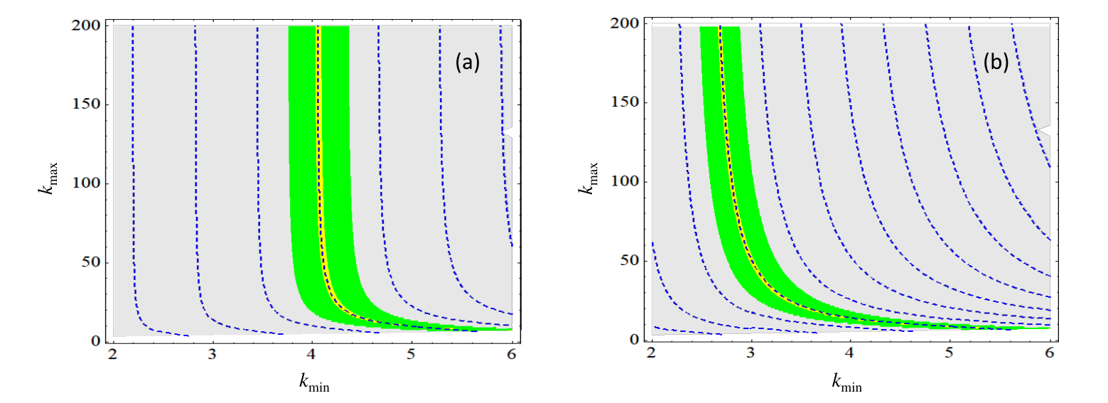
In this context, our goal is to modify the degree distribution to adjust , given the set of parameters . In particular, we will take into consideration that, as we have seen in Fig. 2, a limitation comes from the integer character of , and also from the high probability that the smallest values of have in a pure power-law distribution. Therefore, the schemes that we will propose somehow emulate an analytic continuation between consecutive integer values of , thus allowing to obtain a continuum of values of , overcoming the limitations shown in Fig. Fig. 2.
The proposed schemes are defined in Section II. In Section III, we check that the adjustments of do not introduce undesired correlations in the networks constructed via the configuration model. In Section IV, we describe a procedure to eliminate the fluctuations in the average degree for finite networks. Final considerations are presented in Sec. V.
II Modified degree distribution
Based on the introductory discussion, we propose two simple schemes to adjust the average degree of a power-law network, with given by Eq. (1). These schemes, illustrated in each panel of Fig. 3, consist of modifying the low-degree region of the original . In case I, only the minimal degree does not follow a power-law. In case II, several points can form a plateau, before the power-law decay. Notice that, by altering the shape of low- region, related to the more likely values of , concomitantly the probability associated with the tail increases, allowing for more highly connected nodes. As we will see, this slight modification allows to adjust the average degree.


It is also noteworthy that real degree distributions do not follow a pure power-law but are better represented by the distributions that result from the modified schemes. For example, networks of word co-occurrence, company directors and internet autonomous systems resemble the form of scheme I, while (scientists, film actors) collaboration networks resemble the shape of scheme II newman-chapter.
II.1 Scheme I
Starting from a pure power-law distribution, we scale the probability of the minimal degree by a factor and renormalize the whole distribution, as illustrated in Fig. 3(a). That is
| (3) |
where is the normalization constant. In order to do that, let us consider the parametrization
| (4) |
where and is the floor function. In the particular case , we have and . Increasing between consecutive integer values, makes decrease from 1 to 0. When reaches an integer value, is reset to unit, while increases in one unit. Therefore, when is integer, the pure power-law distribution starting from a minimal degree is recovered. For non-integer , the distribution has the shape illustrated in Fig. 3(a). The plots of the coefficients of the degree distribution and of the average degree, versus the control parameter , are shown in Fig. 4(a). Note that, for given and , tuning allows to change continuously the value of the average degree, which is given by
| (5) |
where and are given by Eqs. (4).

II.2 Scheme II
Another modification of the pure power-law distribution is illustrated in Fig. 3(b), where a plateau (meaning uniform distribution for the lowest degrees) is considered. The modified distribution is
| (6) |
where is the normalization constant.
In this case, there can be more combinations to obtain a given average degree, since there is an additional parameter. In fact, by choosing , the following parametrization controls the length and level of the initial plateau:
| (7) |
where we can take . For , we recover the pure power-law. The behaviors of and with , for , are shown in Fig. 4(b), together with the corresponding average degree
| (8) |
where and are given by Eqs. (7).
III Correlation analysis
Based on the modified degree distributions, we built networks using the configuration model. Self and multiple connections are not frequent in the cases considered and realizations containing such connections were discarded. Similarly, only networks with giant component size were considered.
In order to identify degree-degree correlations, we consider the average degree of the neighbors of a given node , , which in terms of the adjacency matrix , is given by . We compute the average over all nodes with the same degree, ,
| (9) |
where represents the number of nodes with degree . This quantity defines the level of assortativity of the network. If is an increasing (decreasing) function of , the network is assortative (dissassortative). For uncorrelated networks, it is -independent, and given by newman-chapter; serrano2007correlations
| (10) |
We also consider the local clustering coefficient , given by the ratio of the number of existing connections between neighbors of site , (triangles), over its total possible number . If , then . Grouping the local clustering of those vertices with the same degree (as done in Eq. (9)), we have
| (11) |
which in an uncorrelated network is -independent and given by newman
| (12) |


In Fig. 5, we show the theoretical values of and for degree distributions following schemes I (filled symbols) and II (hollow symbols), for two different values of and two values of . Using scheme II, there can be more choices of the minimal degree , since one can tune the length of the plateau, which provides and extra parameter. Notice that the degree distribution of scheme I yields minimal values of and , associated to the reduction of the occurrence of low- nodes.
For the constructed networks, we calculated , the average degree of the neighbors, and the clustering . The results for scheme I are presented in Fig. 6. The horizontal lines correspond to the values predicted for uncorrelated networks. A very good agreement is observed between measured and theoretical values indicating that correlations are not introduced by the correction scheme, as expected. Same agreement is observed for networks constructed with scheme II (not shown).


In Fig. 7, for networks based on scheme I, we show the effect of changing and the structural cut-off , for two values of . Notice that larger produces the increase of and the decrease of . For both network sizes the cut-off (squares) allows to keep nearly constant for all . The cut-off (diamonds) is enough to avoid dependencies for but not in the case where the degree distribution has heavy tails. In fact, in the latter case, a noticeable decay of and with is observed, although this effect is reduced by increasing system size. Actually, this dependency which is nearly linear is always present, but becomes negligible for appropriate . This effect is not a consequence of the introduced schemes, but it is also observed when the degree distribution is a pure power-law UCM.
IV Eliminating fluctuations in the average degree
The two schemes proposed above fulfill the function of controlling the average degree of power-law networks. However, as exemplified in figure 1, the sample average can still fluctuate around the prefixed value , for finite networks. This is because the process by which the sequence of degrees is constructed is purely random. In this subsection, we present a way to eliminate the fluctuations in the average degree. The procedure consists of two steps to chose the sequence of degrees. The first step is deterministic and the second stochastic.
To generate the sequence of degrees, we start from a distribution . The expected value for the number of vertices with degree is , which in general is not an integer value, as it must be for an individual realization. Then, in order to obtain integer number of vertices, we perform a first deterministic step, where we truncate . Then, we add to the list times the degree . This procedure produces fewer vertices and edges than required, which will be corrected in a second stage.
Figure 8(a) shows the intermediate (non-normalized) distribution of degrees after this deterministic process (hence a single realization is shown). For this network we used , and , but the number of vertices was reduced to . As increases, it becomes more evident that , returning values below the original (normalized) degree distribution. Notice that, for large enough , we can have , while for small .


The number of missing nodes is . The degree sequence needs to be completed, to fulfill the desired network size and average degree . The nonnegative fractional part can be used as a filling probability, to draw the remaining elements of the degree sequence, according to the following algorithm:
- 1.
If and , a number is uniformly drawn from the interval , and we decide if it will be added to the sequence or not with probability . Moreover, each value of can be selected only once, then if the drawn value has already been used, a new one is drawn.
- 2.
If after some iterations there is only one missing node, then . In this case, the degree is added to the sequence even if it has been drawn before. The only case in which a repetition is allowed. If the last missing node , then we start it over from step 1.
Figure 8(b) presents the distribution of degrees , after filling the missing nodes generated in panel (a) for a single realization. The average degree is exactly . In the example the degree distribution is a pure power-law but of course the procedure can be applied to any degree distribution.
It is interesting to note that the probability distribution to fill the missing values is nearly uniform up to the value of for which , in which case , hence decaying as a power law for large (see inset). Let us mention that has previously been used to introduce large-degree sites (hubs) via the configuration model in power-law degree distributions maria-BA-congigmodel, although not to control the average degree. Notice that this procedure to eliminate fluctuations is not exclusive of power-law networks and in principle can be applied to any .
V Final remarks
We have analyzed two different modifications of the degree distribution that allow us to adjust the average degree , preserving the power-law character of the distribution. We considered two simple forms of modifying the low- region, but, of course, other shapes might also be used to produce similar results. Additionally, we have presented a procedure to eliminate fluctuations in the average degree, which can be applied to any degree distribution.
Controlling is important since correlations and other structural properties can be affected by the average connectivity ramos2013random; serrano2005tuning. It is particularly relevant when an artificial network is used as a substrate on top of which the dynamics of a complex system evolves. Fixing the average degree in synthetic networks may be also useful for comparisons with real ones, overcoming the difficulties exposed in Ref. brain2010. A further advantage of applying the proposed schemes (either I or II) is that they help to eliminate fragments disconnected from the giant component, as soon as the low values of become less probable. The procedures we proposed to tune the average degree can be directly adapted to adjust the value of other finite moments of the degree distribution.
Let us finally mention that another way to built networks with a power-law degree distribution is using growth techniques. For example, the generalized Barabasi-Albert (GBA) model BA-general allows in principle to adjust the degree-distribution exponent and average degree , for a given size of the network, however there are restrictions in the values that can be achieved (for instance, when , is not possible in GBA). For instance in the particular case of a standard Barabasi-Albert network BA, with , only even values of are obtained in the limit of large . Moreover, although GBA networks present a negligible Pearson coefficient newman-assortative, it is known that these graphs possess -dependencies BA_correlations; rewire_correlations.
We have verified that the modifications introduced in the degree distribution with structural cut-off do not introduce -dependencies in the nearest-neighbor degree and the local clustering coefficient . Although choosing other form of the cutoff may introduce -dependencies, the method to tune is still effective.
We acknowledge partial financial support from Brazilian agencies CAPES (code 001), CNPq and Faperj.
References
- (1) Watts, D. J., A simple model of global cascades on random networks, Proc. Natl. Acad. Sci. USA 99, 5766–5771 (2002).
- (2) M. Ramos, J. Shao, S.D.S. Reis, C. Anteneodo, J.S. Andrade, S. Havlin, H.A. Makse, How does public opinion become extreme?, Sci. Rep. 5, 10032 (2005).
- (3) A.R. Vieira, A.F. Peralta, R. Toral, M. San Miguel, C. Anteneodo, Pair approximation for the noisy threshold -voter model, Phys. Rev. E 101, 052131 (2020).
- (4) A. Mata, R.S. Ferreira, S. C. Ferreira, Heterogeneous pair-approximation for the contact process on complex networks, New Journal of Physics 16, 053006 (2014).
- (5) C.-L. Tang, W.-X. Wang, X. Wu, and B.-H. Wang, Effects of average degree on cooperation in networked evolutionary game, Eur. Phys. J. B 53, 411–415 (2006)
- (6) J. B. de Brito, C. I. N. Sampaio Filho, A. A. Moreira, J. S. Andrade Jr., Characterizing the intrinsic correlations of scale-free networks, Int. J. Mod. Phys. C, 27, 3, 1650024 (2016).
- (7) B.C.M. van Wijk1, C.J. Stam, A. Daffertshofer, Comparing brain networks of different size and connectivity density using graph theory, PLoS ONE 5(10) e13701 (2010).
- (8) M. Molloy, B. Reed, A critical point for random graphs with a given degree sequence, Random Structures & Algorithms. 6 (2–3): 161–180 (1995).
- (9) M. E. J. Newman, Networks: an introduction, (Oxford University Press, Oxford, 2018).
- (10) J. Qu, S. J. Wang, M. Jusup, Z. Wang, Effects of random rewiring on the degree correlation of scale-free networks, Sci. Rep. 5, 15450 (2015).
- (11) S. N. Dorogovtsev, and J. F. F. Mendes, Evolution of networks, Adv. Phys. 51, 1079 (2002).
- (12) M. Catanzaro, M. Boguñá and R. Pastor-Satorras, Generation of uncorrelated random scale-free networks, Phys. Rev. E 71, 027103 (2005).
- (13) M. Boguñá, R. Pastor-Satorras, A. Vespignani, Cut-offs and finite size effects in scale-free networks, Eur. Phys. J. B 38, 205–209 (2004)
- (14) M. E. J. Newman, in Handbook of Graphs and Networks: From the Genome to the Internet, edited by S. Bornholdt and H. G. Schuster (Wiley-VCH, Berlin, 2003), pp. 35–68.
- (15) M. A. Serrano, M. Boguñá, R. Pastor-Satorras, A. Vespignani, Large scale structure and dynamics of complex networks: From information technology to finance and natural sciences (World Scientific Publishing Co. Ltd), pages 35–65 (2007).
- (16) M. L. Bertotti and G. Modanese, The configuration model for Barabasi-Albert networks, Applied Network Science 4, 32 (2019)
- (17) M. Ramos, C. Anteneodo, Random degree–degree correlated networks, Journal of Statistical Mechanics: Theory and Experiment P02024 (2013).
- (18) M. A. Serrano and M. Boguñá, Tuning clustering in random networks with arbitrary degree distributions Phys. Rev. E 72, 036133 (2005).
- (19) R. Albert and A.L. Barabási, Topology of Evolving Networks: Local Events and Universality, Phys. Rev. Lett. 85, 5234 (2000).
- (20) A.L. Barabási,R. Albert , Emergence of scaling in random networks, Science 286 (5439), 509 (1999).
- (21) M. E. J. Newman, Assortative Mixing in Networks, Phys. Rev. Lett. 89, 208701 (2002).
- (22) B. Fotouhi and M. G. Rabbat, Degree correlation in scale-free graphs, Eur. Phys. J. B 86, 510 (2013).