Adaptive Patch Exiting for Scalable Single Image Super-Resolution

Shizun Wang Thanks: Equal Contribution Affiliation: Beijing University of Posts and Telecommunications Jiaming Liu Affiliation: Peking University Kaixin Chen Affiliation: Beijing University of Posts and Telecommunications Xiaoqi Li Affiliation: Peking University Affiliation: OPPO Research Institute E-mail wangshizun@bupt.edu.cn, lu199192@gmail.com Ming Lu Thanks: Corresponding Author Affiliation: Intel Labs China Yandong Guo Affiliation: OPPO Research Institute E-mail wangshizun@bupt.edu.cn, lu199192@gmail.com

Abstract

Since the future of computing is heterogeneous, scalability is a crucial problem for single image super-resolution. Recent works try to train one network, which can be deployed on platforms with different capacities. However, they rely on the pixel-wise sparse convolution, which is not hardware-friendly and achieves limited practical speedup. As image can be divided into patches, which have various restoration difficulties, we present a scalable method based on Adaptive Patch Exiting (APE) to achieve more practical speedup. Specifically, we propose to train a regressor to predict the incremental capacity of each layer for the patch. Once the incremental capacity is below the threshold, the patch can exit at the specific layer. Our method can easily adjust the trade-off between performance and efficiency by changing the threshold of incremental capacity. Furthermore, we propose a novel strategy to enable the network training of our method. We conduct extensive experiments across various backbones, datasets and scaling factors to demonstrate the advantages of our method. Code is available at https://github.com/littlepure2333/APE.

Keywords:

Single Image Super-Resolution, Scalability, Efficiency

1 Introduction

Super-Resolution (SR) is an important technique and has been widely used in video compression [8], rendering acceleration [20], network streaming [23], medical imaging [18], computational photography [19] and so on. As the development of Deep Neural Networks (DNNs), plenty of DNN-based methods are proposed for Single Image Super-Resolution (SISR) [16, 4, 14, 28, 9, 13, 27]. Existing methods mostly cascade convolutional layers many times to construct deep networks and adopt the pixel-shuffle layer [16] to obtain high-resolution output. The cascaded layers increase the network’s capacity of modeling contextual information over larger image regions. Although significant improvements have been made in performance or efficiency over the past few years, the trade-off between performance and efficiency is still under-explored to the best of our knowledge.

Since there are various hardware platforms like CPUs, GPUs, FPGAs and so on, training one scalable network that can be deployed on platforms with different capacities is strongly demanded for future heterogeneous computing. Recently, a pixel-wise adaptive inference method for scalable SISR has been proposed [15]. It learns a predictor to generate the pixel-wise depth map that indicates the target number of layers for each pixel. Sparse convolution guided by the pixel-wise depth map is implemented to achieve speedup. The scalability of [15] is realized by changing the mean average of layers for all pixels. However, although [15] can obtain theoretical FLOPs reduction, the practical speedup is limited since the pixel-wise sparse convolution is not hardware-friendly. Inspired by the fact that image can be divided into patches, which have various restoration difficulties, [10] proposes a general framework that applies appropriate networks to different patches. A module is learned to classify the patches into various restoration difficulties. They train several models with different capacities to super-resolve patches with different difficulties. Although [10] can save up to 50% FLOPS on benchmarking datasets, we observe it has two limitations. Firstly, it applies one fixed network to a certain restoration difficulty, which cannot adjust the trade-off between performance and efficiency as [15]. Secondly, it needs to store one network for each restoration difficulty, heavily increasing the model size.

To solve the above limitations, we present a scalable method based on Adaptive Patch Exiting (APE) for SISR. Our method can train one network to adaptively super-resolve patches with different difficulties. To be more specific, we train a regressor to predict the incremental capacity of each layer for the input patch. The incremental capacity can evaluate the necessity of each layer. Once the incremental capacity is below a threshold, the patch can exit at the specific layer. Our method can easily adjust the trade-off between performance and efficiency by changing the threshold of incremental capacity. On platforms with high computational resources, our method can lower the threshold to utilize more layers for super-resolution. On platforms with low computational resources, our method can raise the threshold to make the patches exit earlier. Therefore, our method is scalable over platforms with different computational resources. Compared with [10], which classifies the patches into certain restoration difficulties, our method enables the scalability by adjusting the threshold. In addition, our method only needs to store one network for all restoration difficulties, significantly reducing the model size.

In order to enable the network training, we further propose a strategy that can jointly train the regressor and SR network. Our strategy first train the multi-exit SR network based on the original network, then we calculate the target incremental capacity of each layer based on the multi-exit SR network. Finally, we jointly train the SR network and regressor to converge.

Our contributions can be concluded as follows:

•

We present a novel scalable method for SISR based on adaptive patch exiting, which can be deployed on platforms with different capacities.
•

We propose to learn the incremental capacity of each layer instead of patch difficulty, enabling the patch to exit at the optimal layer.
•

We introduce an effective joint training strategy to enable the training of incremental capacity regressor and SR network.
•

We conduct detailed experiments across various SR backbones and scaling factors to demonstrate the advantages of our method over existing approaches.

2 Related Work

Single Image Super-Resolution Since the seminal work SRCNN [4], which first applies DNN to SISR, many methods have been proposed. For example, VDSR [9] adopts a very deep neural network to learn the image residual. EDSR [14] analyzes the DNN layers and proposes to remove some redundant layers from SRResNet [11]. RDN [29] uses dense connections that fully utilize the information of preceding layers. RCAN [28] explores the attention mechanism and proposes attentive DNNs to boost the performance. In order to reduce the computational cost, FSRCNN [5] and ESPCN [16] propose to use LR image as input and upscale the feature map at the end of networks. LAPAR [12] presents a method based on linearly-assembled pixel-adaptive regression network, which learns the pixel-wise filter kernel. In addition to methods focusing on network design, many works study the real-world SR problem. RealSR [3] builds a real-world dataset with paired LR-HR images captured by adjusting the focal length. They also present a Laplacian pyramid-based kernel prediction network to recover the HR image. Zero-Shot SR [17] exploits the power of DNN without relying on prior training. They train a small image-specific DNN at test time on examples extracted from the input image itself. Recently, the community also shows the trend of applying techniques like network pruning, quantization, distillation, AutoML to SR. BSRN [21] designs a bit-accumulation mechanism to approximate the full-precision convolution with a value accumulation scheme. Although plenty of DNN-based methods are proposed to improve the performance or efficiency, the scalability problem is still under-explored to the best of our knowledge.

Adaptive Inference Since the future of computing is heterogeneous, training one scalable network that can be deployed on platforms with different capacities is a very important problem. [26] proposes a simple method that trains a single network executable at different widths, enabling instant and adaptive performance-efficiency trade-off at runtime. [25] further extends the slimmable networks [26] from a predefined widths set to arbitrary width, and generalizes to networks both with and without batch normalization layers. [24] presents a method that trains a single slimmable network to approximate the network performance of different channel configurations, and then searches the optimized channel configurations under different resource constraints. Instead of switching network width, [7] investigates the option that achieves instant and flexible deployment by adaptive bit-widths of weights and activations in the model. [22] trains a set of sub-networks with different widths using different input resolutions to mutually learn multi-scale representations for each sub-network. The performance-efficiency trade-off can be achieved by changing both the network width and input resolution. [2] proposes to train a once-for-all network that supports diverse platforms by decoupling training and search. They can quickly get a specialized sub-network by selecting from the once-for-all network without additional training. Although plenty of methods are proposed for adaptive inference, they mainly focus on high-level vision tasks. The scalability problem of low-level vision tasks is still under-explored as far as we know. Inspired by the fact that different image regions have different restoration difficulties, [15] introduces a lightweight adapter module, which takes image features and resource constraints as input and predicts a pixel-wise depth map. Therefore, only a fraction of the layers in the backbone is performed at a given position according to the predicted depth. While [15] can achieve theoretical FLOPS reduction, the practical speed gain is limited since unstructured sparse convolution is not hardware friendly. [10] also utilizes the properties of different image regions by dividing the images into local patches. They train a module to classify the patches into different difficulties, and apply appropriate model to each difficulty. Although [10] can obtain practical speed gains, it is not scalable under different resource constraints.

3 Method

To apply Adaptive Patch Exiting (APE) to existing SR networks, we modify the original SR networks to multi-exit networks and present the training strategy in Sec. 3.1. We then analyze the performance of each patch at a certain layer, and introduce the incremental capacity to evaluate the necessity of each layer for a patch in Sec. 3.2. Finally, we jointly train the SR network and lightweight regressor in Sec. 3.3. The regressor is used to estimate the incremental capacity at a certain layer. The trained network can achieve the trade-off between performance and efficiency by adjusting the threshold of incremental capacity. The overall pipeline is illustrated in Fig. 1.

Refer to caption — Figure 1: The pipeline of Adaptive Patch Exiting (APE). Original SR networks take a LR image as input, and forward it through head, body and tail to generate the SR image. Instead, APE first splits the LR image into patches, which are forwarded in parallel. The patches will exit early if the incremental capacity estimated by the regressor is below a given threshold. Finally, the SR patches are merged to the output image.

3.1 Training Multi-Exit SR Networks

Super-resolution aims to recover a High-Resolution (HR) image $\hat{y}$ from a given Low-Resolution (LR) image $x$ . Since the pioneering work [4], most of the SR networks consist of three parts: head, body and tail. The head part $H$ extracts the features $f_{0}$ from the LR image:

f_{0}=H(x;\Theta_{h})

(1)

and the body part $B$ enhances $f_{0}$ by cascading $N$ convolutional layers to generate feature $f_{N}$ :

f_{N}=B(f_{0};\Theta_{b})

(2)

Finally, the tail part $T$ takes the enhanced feature $f_{N}$ to obtain the SR output $\hat{y}$ :

\hat{y}=T(f_{N};\Theta_{t})

(3)

where $\Theta_{h}$ , $\Theta_{b}$ and $\Theta_{t}$ denote the parameters of head, body and tail individually. Typical SISR architectures such as EDSR [14], RCAN [28], VDSR [9] and ECBSR [27] all follow this pipeline. We denote the original SR network as $F$ :

\hat{y}=F(x;\Theta_{h},\Theta_{b},\Theta_{t})=T(B(H(x;\Theta_{h});\Theta_{b});\Theta_{t})

(4)

Without any change to head and tail, we can simply modify the number of repeated layers in the body to change the network capacity. We extract the intermediate feature ${f_{i}}$ of the body, where $i\in[1,N]$ , to generate the early-exit output:

\widehat{{y_{i}}}=T({f_{i}};{\Theta_{t}})

(5)

The original SR network uses the last layer’s feature ${f_{N}}$ to generate the output. As the intermediate features of body have the same resolution as last layer’s feature, we construct the multi-exit SR network by exit early in the intermediate layers. Different exits require different computational resources. We initialize the multi-exit SR network with the pre-trained model, and all exits’ L1 losses are summed up as the multi-exit SR network’s reconstruction loss $L_{m}$ :

L_{m}=\sum_{i=1}^{N}|\hat{y_{i}}-y|

(6)

where ${y}$ represents the HR image and $N$ is the total number of layers. The training details are identical to the setup described in Sec. 4.1.

3.2 Estimating Incremental Capacity

In order to make the multi-exit SR networks scalable, we need to design the signal of early-exit at a certain layer. Therefore, we train a 32-exit EDSR on DIV2K, and randomly sample 32 × 32 LR patches to observe their layer-wise performances. The result is shown in Fig. 2(a). A naive method of adaptive inference is to exit early when the performance is exceeding a threshold. However, we observe that there are three types of patches. The first one is named as bottleneck patches, which can achieve satisfying performance with a few layers as shown in Fig. 2(b). The second one is called growing patches, which need more layers to achieve good performance as shown in Fig. 2(c). The third one is called over-fitting patches as shown in Fig. 2(d), which might even achieve worse performance with more layers. In addition, the intervals of these three types are also quite different. The above observation shows that the signal of early-exit should be released when the performance gets saturated, rather than when the performance exceeding a threshold.

We define the early-exit signal $I_{i}$ as the incremental capacity of ${i^{th}}$ layer, which measures the performance difference between current layer and previous layer:

I_{i}=\sigma(P_{i}-P_{i-1})

(7)

where $\sigma$ is the tanh function, $P_{i}$ is the reconstruction performance of ${i^{th}}$ layer. As can be seen, the range of $I_{i}$ is $[-1,1]$ . Higher incremental capacity means more performance gain when forwarding ${i^{th}}$ layer. When $I_{i}$ is close to $0$ , it means the performance get saturated. When $I_{i}$ is below $0$ , it indicates the performance will get worse. In this paper, we use the PSNR between SR image and HR image as the reconstruction performance:

P_{i}=PSNR(\hat{y_{i}},y)

(8)

[10] proposes to train a module to classify the patches into different difficulties. However, as we have mentioned above, the relation between network capacity and performance is not monotonic. There are some patches that achieve worse results with more layers. Instead, using the incremental capacity can always correctly measure the saturation of performance and exit at the optimal layer.

During inference, since we cannot get the accurate incremental capacity due to the lack of HR image. Therefore, we propose to train a lightweight regressor $R$ , which takes the feature $f_{i}$ of each layer in the body as input, to estimate the ${i^{th}}$ layer’s incremental capacity $\hat{I_{i}}$ . All the layers share the same regressor:

\hat{I_{i}}=\sigma(W\ast g(f_{i})+b)

(9)

The regressor contains a fully-connected layer, where $g$ is global average pooling operation, $W$ and $b$ are the weight and bias of the fully-connected layer. The loss function of the regressor is the L2 loss between $\hat{I_{i}}$ and ground-truth incremental capacity $I_{i}$ :

L_{i}={\parallel}\hat{I_{i}}-I_{i}{\parallel}_{2}^{2}

(10)

3.3 Jointly Training SR Network and Regressor

To apply APE to a SR network, we train its multi-exit SR network and the regressor jointly. The overall loss consists of all layers’ reconstruction loss and the incremental capacity regression loss:

L=L_{m}+\lambda\sum_{i=1}^{N}L_{i}

(11)

where $\lambda$ is a hyper-parameter to balance these two losses, and we set it to 1 for all our experiments. During inference, we split the input image into overlapped patches, and feed all the patches into multi-exit SR network in parallel. Once the incremental capacity of a patch is below a given threshold, the patch can exit early. Increasing the threshold will make patches exit earlier and reduce the computational cost. Finally, the HR patches are merged to obtain the output image.

4 Experiments

4.1 Implementation Details

Training Setup

We use DIV2K dataset [1] to train all the models. The low-resolution images are generated by bicubic downsampling with scaling factors $\times 2$ , $\times 3$ and $\times 4$ . Following former works, we use the first 800 images as the training set and 10 images (0801-0810) as the validation set. During training, data augmentation including random horizontal flip, random vertical flip and 90^∘ rotation are applied. We train all the models for 300 epochs with learning rate initialed as 1e-4 and decayed to half at 200 epochs. The batch size is 16 and the HR patch size is 192. We use Adam optimizer, where $\beta_{1}$ is set to 0.9 and $\beta_{2}$ is set to 0.999.

Testing Setup

We use DIV2K [1] dataset and DIV8K [6] dataset for testing since the widely-used benchmark datasets are not suitable for large image super-resolution evaluation. Specifically, we choose 100 images (0801-0900) from DIV2K for high-definition (HD) scenario, and 100 images (1401-1500) from DIV8K for ultra high-definition (UHD) scenario. During testing, we first split LR images into patches of size 48 with stride 46 unless otherwise specified. Then the LR patches are super-resolved in parallel, and the parallel size can be tuned to fit the computational resource. Finally, the SR patches are merged to obtain the complete SR images by weighting overlapping areas. The Peak Signal-to-Noise Ratio (PSNR) and Structural Similarity (SSIM) calculated on RGB channels are adopted as the evaluation metrics to measure super-resolution performance. We use FLOPs to evaluate the computational cost and the practical running time is benchmarked on NVIDIA 2080Ti GPUs.

Table 1: Performance evaluation of APE. FLOPs, PSNR and SSIM on DIV2K and DIV8K datasets with scaling factors

\times 2

\times 3

\times 4

are reported in the table. To compare the performance of APE with baselines, incremental capacity threshold is set to

0

. Therefore, all the patches can exit at the optimal layers.

Method	Scale	DIV2K			DIV8K
Method	Scale	FLOPS	PSNR	SSIM	FLOPS	PSNR	SSIM
ECBSR	$\times 2$	1.38G	33.86dB	0.9309	1.38G	39.82dB	0.9649
ECBSR-APE	$\times 2$	1.37G	33.87dB	0.9316	1.37G	39.73dB	0.9646
VDSR	$\times 2$	6.17G	33.63dB	0.9286	6.17G	39.71dB	0.9640
VDSR-APE	$\times 2$	6.14G	33.62dB	0.9292	6.15G	39.54dB	0.9636
RCAN	$\times 2$	35.36G	34.09dB	0.9330	35.36G	40.04dB	0.9657
RCAN-APE	$\times 2$	35.36G	34.36dB	0.9357	35.36G	40.22dB	0.9663
EDSR	$\times 2$	93.89G	34.21dB	0.9343	93.89G	39.97dB	0.9656
EDSR-APE	$\times 2$	93.89G	34.46dB	0.9366	93.89G	40.16dB	0.9662
ECBSR	$\times 3$	1.40G	30.22dB	0.8606	1.40G	35.36dB	0.9158
ECBSR-APE	$\times 3$	1.40G	30.16dB	0.8618	1.40G	35.31dB	0.9159
VDSR	$\times 3$	13.88G	29.99dB	0.8567	13.88G	35.15dB	0.9133
VDSR-APE	$\times 3$	13.88G	29.92dB	0.8574	13.88G	35.15dB	0.9138
RCAN	$\times 3$	35.80G	30.45dB	0.8645	35.80G	35.44dB	0.9171
RCAN-APE	$\times 3$	35.74G	30.59dB	0.8695	35.76G	35.65dB	0.9192
EDSR	$\times 3$	100.77G	30.55dB	0.8669	100.77G	35.54dB	0.9178
EDSR-APE	$\times 3$	100.77G	30.66dB	0.8711	100.77G	35.68dB	0.9197
ECBSR	$\times 4$	1.43G	28.29dB	0.8026	1.43G	33.07dB	0.8724
ECBSR-APE	$\times 4$	1.43G	28.31dB	0.8036	1.43G	33.05dB	0.8719
VDSR	$\times 4$	24.68G	28.12dB	0.7974	24.68G	32.88dB	0.8688
VDSR-APE	$\times 4$	24.53G	28.10dB	0.7991	24.53G	32.83dB	0.8689
RCAN	$\times 4$	36.77G	28.52dB	0.8077	36.77G	33.25dB	0.8753
RCAN-APE	$\times 4$	36.71G	28.70dB	0.8138	36.74G	33.38dB	0.8776
EDSR	$\times 4$	115.83G	28.66dB	0.8112	115.83G	33.30dB	0.8762
EDSR-APE	$\times 4$	115.79G	28.78dB	0.8158	115.81G	33.39dB	0.8779

Table 2: Efficiency evaluation of APE under the same performance as original SR networks. Parameters, body FLOPs, total FLOPs, and practical inference times on DIV2K with scaling factors

\times 2

\times 3

\times 4

are reported in the table. Inference time is evaluated on NVIDIA 2080Ti GPUs.

Method	Scale	Param.	PSNR	Body FLOPs	Total FLOPs	Time (ms)
ECBSR	$\times 2$	1.0K	33.86dB	1.36G	1.38G (100%)	244
ECBSR-APE	$\times 2$	1.0K	33.82dB	0.99G	1.01G (73%)	211
VDSR	$\times 2$	0.67M	33.63dB	6.14G	6.17G (100%)	346
VDSR-APE	$\times 2$	0.67M	33.61dB	4.13G	4.16G (67%)	334
RCAN	$\times 2$	15.4M	34.09dB	34.91G	35.36G (100%)	2323
RCAN-APE	$\times 2$	15.4M	34.09dB	8.26G	8.71G (24%)	974
EDSR	$\times 2$	40.7M	34.21dB	87.01G	93.89G (100%)	2133
EDSR-APE	$\times 2$	40.7M	34.21dB	34.07G	40.95G (43%)	733
ECBSR	$\times 3$	1.0K	30.21dB	1.36G	1.40G (100%)	239
ECBSR-APE	$\times 3$	1.0K	30.12dB	1.01G	1.05G (74%)	219
VDSR	$\times 3$	0.67M	29.99dB	13.80G	13.88G (100%)	346
VDSR-APE	$\times 3$	0.67M	29.91dB	11.01G	11.09G (79%)	325
RCAN	$\times 3$	15.6M	30.45dB	34.91G	35.80G (100%)	1040
RCAN-APE	$\times 3$	15.6M	30.45dB	13.57G	14.46G (40%)	627
EDSR	$\times 3$	43.7M	30.55dB	87.01G	100.77G (100%)	1777
EDSR-APE	$\times 3$	43.7M	30.55dB	49.28G	63.04G (62%)	492
ECBSR	$\times 4$	1.0K	28.29dB	1.36G	1.43G (100%)	245
ECBSR-APE	$\times 4$	1.0K	28.22dB	0.85G	0.92G (64%)	196
VDSR	$\times 4$	0.67M	28.12dB	24.55G	24.68G (100%)	345
VDSR-APE	$\times 4$	0.67M	28.07dB	17.75G	17.88G (72%)	303
RCAN	$\times 4$	15.6M	28.53dB	34.91G	36.77G (100%)	620
RCAN-APE	$\times 4$	15.6M	28.53dB	10.53G	12.39G (33%)	350
EDSR	$\times 4$	43.1M	28.66dB	87.01G	115.83G (100%)	1123
EDSR-APE	$\times 4$	43.1M	28.67dB	49.86G	78.68G (67%)	419

4.2 Evaluation of APE

Performance Results

To evaluate the effectiveness of our method, we apply APE to state-of-the-art SR networks, including ECBSR [27], VDSR [9], EDSR [14] and RCAN [28]. We set the threshold of incremental capacity to 0 and evaluate the performance of APE on DIV2K and DIV8K. As we have mentioned above, there are three types of patches. The over-fitting patches might achieve worse performance with more layers. Therefore, setting the threshold to 0 enables all the patches to exit at the optimal layers. As shown in Tab. 1, SR networks with APE can achieve comparable or even superior performance compared to original SR networks in terms of PSNR and SSIM. This comparison demonstrates that incremental capacity is a more reasonable metric to evaluate the contribution of each layer.

Efficiency Results

As for the efficiency of APE, Tab. 2 shows the detailed computational cost under same performance as original SR networks. Our method adds a lightweight regressor whose FLOPs is negligible. APE can significantly reduce the computational cost of original SR networks across different scaling factors. For example, RCAN-APE only needs 24%, 40%, and 33% of original computational cost on scaling factors $\times 2$ , $\times 3$ and $\times 4$ . The computational cost of body is significantly reduced by our method, and the computational costs of head and tail stay the same. Overall, our method can nearly halve the computational cost under the same performance.

Scalability Results

We also show the performance-efficiency trade-off results in Fig. 3 to demonstrate the scalability of APE. By controlling the incremental capacity threshold, APE can achieve scalable performance-efficiency trade-off. Therefore, we can deploy one APE SR network on platforms with different computational resources. For the device with low computational resource, we can raise the threshold to get lower performance and faster inference speed.

(a) PSNR-GFLOPs on DIV2K

\times 2

(b) SSIM-GFLOPs on DIV2K

\times 2

\times 4

(d) SSIM-GFLOPs on DIV2K

\times 4

Figure 3: Quantitative results of performance-efficiency trade-off. We apply APE to ECBSR, VDSR, EDSR and RCAN with scaling factors

\times 2

and

\times 4

on DIV2K dataset. Average FLOPs of all 48

\times

48 LR patches and PSNR/SSIM calculated on the full image are reported.

Visual Results

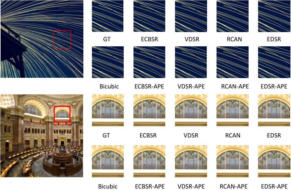
Fig. 4 shows the qualitative comparison of our method against the original SR networks. As we can see, EDSR-APE and RCAN-APE can achieve same or even better visual results compared with original SR networks. Although we merge the patches to obtain complete SR images, weighting overlapped patches can avoid the stitching artifacts.

Fig. 5 visualizes the status of adaptive exiting patches. As can be seen, most patches in smooth regions exit at the early layers since they are easy to be restored. As for patches in complicated regions, they will exit at the later layers. This is consistent with the motivation of applying appropriate networks to various difficulties.

4.3 Ablation Study

Variants of Exit Interval

We conduct the experiment to study the influence of different exit intervals using EDSR as the backbone. Specifically, EDSR has 32 repeated residual layers in the body. We evaluate the exit intervals of 4, 2 and 1 layers. The results on DIV2K dataset with scaling factors $\times 2$ are shown in Fig. 7. As can be seen, exit interval of 4 layers achieves the best results, indicating that multi-exit SR networks need sufficient learning capacity within each exit.

Figure 6: Variants of exit interval. We show the results of different exit intervals by evaluating EDSR-APE on the DIV2K dataset with scaling factors

\times 2

. APE-

n

means APE with

n

exits.

Figure 7: Variants of early-exit signal.

IC

denotes incremental capacity, and

AP

denotes absolute performance. Both are evaluated on DIV2K dataset with

\times 2

scaling factor.

Variants of Early-Exit Signal

Apart from the proposed incremental capacity ( $IC$ ), we can also use the absolute performance ( $AP$ ) of each layer as the early-exit signal to measure the necessity of early-exiting at specific layer. We compare the results of incremental capacity and absolute performance in Fig. 7. As can be seen, compared with absolute performance, incremental capacity can reduce more computational cost, validating that incremental capacity is the better early-exit signal for multi-exit SR networks.

Variants of Patch Size and Stride

Since our method splits an image into patches, we evaluate the performance of different patch sizes and strides. As shown in Tab. 4, different patch size can achieve similar performance in terms of PSNR and SSIM.

4.4 Comparison with ClassSR and AdaDSR

We also compare with ClassSR [10] and AdaDSR [15] on DIV2K $\times 4$ using RCAN as the backbone under the same performance in Tab. 4. We use the published codes of AdaDSR and ClassSR to perform the comparison. ClassSR [10] is a patch-based SR method. It manually designs easy, medium and hard networks by changing the number of channels. A module is trained to classify the patches into easy, medium and hard. ClassSR [10] can reduce the overall computational cost by applying different networks to different patches. However, they need to store all the models with different capacities, heavily increasing the model size. Apart from this, ClassSR classifies the patches into certain restoration difficulties. Therefore, it is not scalable over different computational resources. Instead, our method can easily adjust the trade-off between performance and efficiency to meet different computational resources.

Table 3: Variants of patch size and stride. PSNR and SSIM are evaluated on DIV2K dataset with scaling factor

\times 4

. The numbers in the Patch column indicate (patch size, patch stride).

Method	Patch	PSNR	SSIM
EDSR	-	28.66	0.8112
EDSR-APE	(32,30)	28.702	0.8136
EDSR-APE	(40,38)	28.723	0.8151
EDSR-APE	(48,46)	28.783	0.8158

Table 4: Comparison with AdaDSR and ClassSR, APE achieves fastest inference speed without increasing the model’s size. Besides, APE is scalable to different computational resources.

Method	Param.	PSNR	Time
RCAN	15.6M	28.526	620ms
RCAN-APE	15.6M	28.530	350ms
RCAN-Ada	15.7M	28.535	1644ms
RCAN-ClassSR	30.1M	28.533	22s

We also compare with AdaDSR [15], which is based on pixel-wise sparse convolution. It will generate a spatially sparse mask for each layer and sparse convolution is conducted to achieve speedup. However, pixel-wise sparse convolution is not hardware-friendly on modern GPUs, thus there exists a gap between theoretical and practical speedup. As can be seen in Tab. 4, with similar model size, APE is faster than AdaDSR in practice.

5 Future Work

Although our method can decide the optimal exit for each patch, we still rely on overlapped patches to avoid the stitching artifacts. Therefore, we can further improve the efficiency by adopting non-overlapped patches. Besides, we uniformly split an image into patches, which might not be the optimal solution for image splitting. Finally, applying our method to other low-level vision tasks is also a promising future work.

6 Conclusion

In this paper, we present adaptive patch exiting (APE) for scalable single image super-resolution. Since image patches are structured and have different restoration difficulties, we split an image into patches and train a regressor to predict the incremental capacity of each layer for the input patch. Therefore, the patch can exit at any layer by adjusting the threshold. We also propose a novel joint training strategy to train both the SR network and regressor. Extensive comparisons are conducted across various SR backbones, datasets and scaling factors to demonstrate the effectiveness of our method.

References

[1] Agustsson, E., Timofte, R.: Ntire 2017 challenge on single image super-resolution: Dataset and study. In: The IEEE Conference on Computer Vision and Pattern Recognition (CVPR) Workshops (July 2017)
[2] Cai, H., Gan, C., Wang, T., Zhang, Z., Han, S.: Once-for-all: Train one network and specialize it for efficient deployment. arXiv preprint arXiv:1908.09791 (2019)
[3] Cai, J., Zeng, H., Yong, H., Cao, Z., Zhang, L.: Toward real-world single image super-resolution: A new benchmark and a new model. In: Proceedings of the IEEE/CVF International Conference on Computer Vision. pp. 3086–3095 (2019)
[4] Dong, C., Loy, C.C., He, K., Tang, X.: Learning a deep convolutional network for image super-resolution. In: European conference on computer vision. pp. 184–199. Springer (2014)
[5] Dong, C., Loy, C.C., Tang, X.: Accelerating the super-resolution convolutional neural network. In: European conference on computer vision. pp. 391–407. Springer (2016)
[6] Gu, S., Lugmayr, A., Danelljan, M., Fritsche, M., Lamour, J., Timofte, R.: Div8k: Diverse 8k resolution image dataset. In: 2019 IEEE/CVF International Conference on Computer Vision Workshop (ICCVW). pp. 3512–3516. IEEE (2019)
[7] Jin, Q., Yang, L., Liao, Z.: Adabits: Neural network quantization with adaptive bit-widths. In: Proceedings of the IEEE/CVF Conference on Computer Vision and Pattern Recognition. pp. 2146–2156 (2020)
[8] Khani, M., Sivaraman, V., Alizadeh, M.: Efficient video compression via content-adaptive super-resolution. arXiv preprint arXiv:2104.02322 (2021)
[9] Kim, J., Kwon Lee, J., Mu Lee, K.: Accurate image super-resolution using very deep convolutional networks. In: Proceedings of the IEEE conference on computer vision and pattern recognition. pp. 1646–1654 (2016)
[10] Kong, X., Zhao, H., Qiao, Y., Dong, C.: Classsr: A general framework to accelerate super-resolution networks by data characteristic. In: Proceedings of the IEEE/CVF Conference on Computer Vision and Pattern Recognition. pp. 12016–12025 (2021)
[11] Ledig, C., Theis, L., Huszár, F., Caballero, J., Cunningham, A., Acosta, A., Aitken, A., Tejani, A., Totz, J., Wang, Z., et al.: Photo-realistic single image super-resolution using a generative adversarial network. In: Proceedings of the IEEE conference on computer vision and pattern recognition. pp. 4681–4690 (2017)
[12] Li, W., Zhou, K., Qi, L., Jiang, N., Lu, J., Jia, J.: Lapar: Linearly-assembled pixel-adaptive regression network for single image super-resolution and beyond. Advances in Neural Information Processing Systems 33 (2020)
[13] Li, W., Zhou, K., Qi, L., Jiang, N., Lu, J., Jia, J.: Lapar: Linearly-assembled pixel-adaptive regression network for single image super-resolution and beyond. arXiv preprint arXiv:2105.10422 (2021)
[14] Lim, B., Son, S., Kim, H., Nah, S., Mu Lee, K.: Enhanced deep residual networks for single image super-resolution. In: Proceedings of the IEEE conference on computer vision and pattern recognition workshops. pp. 136–144 (2017)
[15] Liu, M., Zhang, Z., Hou, L., Zuo, W., Zhang, L.: Deep adaptive inference networks for single image super-resolution. In: European Conference on Computer Vision. pp. 131–148. Springer (2020)
[16] Shi, W., Caballero, J., Huszár, F., Totz, J., Aitken, A.P., Bishop, R., Rueckert, D., Wang, Z.: Real-time single image and video super-resolution using an efficient sub-pixel convolutional neural network. In: Proceedings of the IEEE conference on computer vision and pattern recognition. pp. 1874–1883 (2016)
[17] Shocher, A., Cohen, N., Irani, M.: “zero-shot” super-resolution using deep internal learning. In: Proceedings of the IEEE Conference on Computer Vision and Pattern Recognition. pp. 3118–3126 (2018)
[18] Sui, Y., Afacan, O., Gholipour, A., Warfield, S.K.: Learning a gradient guidance for spatially isotropic mri super-resolution reconstruction. In: International Conference on Medical Image Computing and Computer-Assisted Intervention. pp. 136–146. Springer (2020)
[19] Wronski, B., Garcia-Dorado, I., Ernst, M., Kelly, D., Krainin, M., Liang, C.K., Levoy, M., Milanfar, P.: Handheld multi-frame super-resolution. ACM Transactions on Graphics (TOG) 38(4), 1–18 (2019)
[20] Xiao, L., Nouri, S., Chapman, M., Fix, A., Lanman, D., Kaplanyan, A.: Neural supersampling for real-time rendering. ACM Transactions on Graphics (TOG) 39(4), 142–1 (2020)
[21] Xin, J., Wang, N., Jiang, X., Li, J., Huang, H., Gao, X.: Binarized neural network for single image super resolution. In: European Conference on Computer Vision. pp. 91–107. Springer (2020)
[22] Yang, T., Zhu, S., Chen, C., Yan, S., Zhang, M., Willis, A.: Mutualnet: Adaptive convnet via mutual learning from network width and resolution. In: European conference on computer vision. pp. 299–315. Springer (2020)
[23] Yeo, H., Chong, C.J., Jung, Y., Ye, J., Han, D.: Nemo: enabling neural-enhanced video streaming on commodity mobile devices. In: Proceedings of the 26th Annual International Conference on Mobile Computing and Networking. pp. 1–14 (2020)
[24] Yu, J., Huang, T.: Autoslim: Towards one-shot architecture search for channel numbers. arXiv preprint arXiv:1903.11728 (2019)
[25] Yu, J., Huang, T.S.: Universally slimmable networks and improved training techniques. In: Proceedings of the IEEE/CVF International Conference on Computer Vision. pp. 1803–1811 (2019)
[26] Yu, J., Yang, L., Xu, N., Yang, J., Huang, T.: Slimmable neural networks. arXiv preprint arXiv:1812.08928 (2018)
[27] Zhang, X., Zeng, H., Zhang, L.: Edge-oriented convolution block for real-time super resolution on mobile devices. In: Proceedings of the 29th ACM International Conference on Multimedia. pp. 4034–4043 (2021)
[28] Zhang, Y., Li, K., Li, K., Wang, L., Zhong, B., Fu, Y.: Image super-resolution using very deep residual channel attention networks. In: Proceedings of the European conference on computer vision (ECCV). pp. 286–301 (2018)
[29] Zhang, Y., Tian, Y., Kong, Y., Zhong, B., Fu, Y.: Residual dense network for image super-resolution. In: Proceedings of the IEEE conference on computer vision and pattern recognition. pp. 2472–2481 (2018)