跳到论文正文
W Papers独立论文阅读器 arXiv:2203.10817 论文正文 计算阅读时间 · 0%
引用这篇论文根据当前论文元数据生成,正式投稿前建议核对。


License: arXiv.org perpetual non-exclusive license
arXiv:2203.10817v3 [math.DS] 22 Nov 2022

Distributed hybrid observer with prescribed convergence rate for a linear plant using multi-hop decomposition

Riccardo Bertollo Affiliation: R. Bertollo is with the University of Trento, Italy (e-mail: riccardo.bertollo@unitn.it).    Pablo Millán Affiliation: P. Millán and L. Orihuela are with Universidad Loyola Andalucía, Spain (e-mail: pmillan,dorihuela@uloyola.es).    Luis Orihuela Affiliation: P. Millán and L. Orihuela are with Universidad Loyola Andalucía, Spain (e-mail: pmillan,dorihuela@uloyola.es).    Alexandre Seuret Affiliation: A. Seuret is with Universidad de Sevilla, Spain (e-mail: aseuret@us.es),    Luca Zaccarian Thanks: Research supported in part by ANR via grant HANDY (number ANR-18-CE40-0010), by project METRICA (Grant PID2020-117800GB-I00 funded by AEI/MCeI) and project IRRIGATE (Grant PY20 RE 017 funded by Junta de Andalucía). Affiliation: L. Zaccarian is with LAAS-CNRS, University of Toulouse, CNRS, Toulouse, France and the University of Trento, Italy (e-mail: lzaccarian@laas.fr).
Abstract

We propose a distributed hybrid observer for a sensor network where the plant and local observers run in continuous time and the information exchange among the sensing nodes is sampled-data. Process disturbances, measurement noise and communication noise are considered, and we prove that under some necessary detectability assumptions the observer gains can be tuned to guarantee exponential Input-to-State Stability with a prescribed convergence rate. Simulations illustrate the performance of the proposed observer.

Index Terms: 
Distributed estimation; Hybrid observer; Linear systems; Input-to-State Stability; Sensor network

I Introduction

One of the most important tasks for a Wireless Sensor Network (WSN) is state estimation, which finds important applications in different applications areas such as robotics, power systems, smart grids or traffic management, among others. In distributed state estimation, each smart sensor (referred usually as agent) estimates the plant state with limited locally available information, possibly coming from seldom information exchange with neighboring agents. Perhaps the most popular approach for this setting is the Distributed Kalman Filter (DKF) [1]. DKF algorithms involve several steps that typically include: i) prediction of prior states using the system model, ii) correction based on local measurements with a Kalman gain, and iii) information fusion from neighboring agents based on consensus [2, 3, 4], diffusion [5], or gossip-based algorithms [6]. An excellent review of these techniques can be found in [7].

Unlike DKF, distributed Luenberger observers do not use statistical noise/disturbance descriptions [8] and resort to deterministic approaches. To solve the problem in a distributed way, different state-based partitions have been proposed. In [9], a new estimation structure based on the observability canonical form is given, which depends on locally measured outputs and an agent indexing or ordering. An alternative subspace decomposition method, called multi-hop decomposition, is proposed in [10], where each agent constructs its own observability staircase form. These works provide a fully distributed design for the estimator in discrete time [8, 9, 10] or continuous time [10]. However, the case where the local measurements are available in continuous time but the communication among the agents happens in discrete time cannot be analyzed with these approaches. That situation, which has been studied only in the centralized case (see e.g. [11, 12, 13] and references therein), is certainly relevant in practice. Indeed, on the one hand, requiring continuous-time communication would be too stringent and, on the other hand, designing sampled-data solutions with a single sampling time forces the algorithm to run at the inter-agent communication rate, typically much slower than the rate at which the local outputs can be locally measured.

This paper develops a new hybrid distributed observer exploiting the multi-hop decomposition [10] for linear plants equipped with a sensor network. Each network node runs locally a hybrid observer in continuous time for the locally observable modes, exploiting the continuous availability of locally measured outputs through continuous Luenberger-like dynamics. Our work exploits the multi-hop decomposition in [10] for the two-time-scale setting of fast local output injection and slow sampled-data inter-agent exchange, in addition to rigorously characterizing the effect of (continuous-time) process disturbance/sensor noise and (discrete-time) communication exchange disturbances. Using an ad-hoc Lyapunov construction (different from [10]), we guarantee a prescribed convergence rate and input-to-state stability (ISS) properties.

Notation: Scalar ai​ja_{ij} denotes the (i,j)(i,j) entry of matrix AA. Given V⊂ℕV\subset\mathbb{N} and an ordered set YiY_{i} of matrices, for decreasing values of ii from top to bottom, we denote by diagi∈V⁡(Yi)\diag\nolimits\limits_{i\in V}\left(Y_{i}\right) a block diagonal matrix whose diagonal blocks are YiY_{i}, while for the case where matrices YiY_{i} all have the same number of columns, coli∈V⁡(Yi)\col\nolimits\limits_{i\in V}\left(Y_{i}\right), where V⊂ℕV\subset\mathbb{N} and YiY_{i} a matrix vertically stacking YiY_{i}. We often denote (u,v):=[u⊤,v⊤]⊤\left(u,v\right):=\left[u^{\top},v^{\top}\right]^{\top}. |x|:=x⊤​x|x|:=\sqrt{x^{\top}x} is the Euclidean norm of vector xx. ‖x‖∞\|x\|_{\infty} denotes the ℒ\mathcal{L}-infinity norm of the signal x⁡(⋅)x(\cdot). Given two sets 𝒱⊂ℕ\mathcal{V}\subset\mathbb{N} and ℰ⊂𝒱×𝒱\mathcal{E}\subset\mathcal{V}\times\mathcal{V}, 𝒢⁡(𝒱,ℰ)\mathcal{G}(\mathcal{V},\mathcal{E}) is the (directed) graph with nodes 𝒱\mathcal{V} and edges ℰ\mathcal{E}. Finally, 𝒩i\mathcal{N}_{i} denotes the set of nodes jj such that (j,i)(j,i) is an edge of 𝒢⁡(𝒱,ℰ)\mathcal{G}(\mathcal{V},\mathcal{E}), called in-neighborhood of node ii.

II System description and problem formulation

II-A System data

Consider a linear plant subject to an external disturbance driven by the following equation

x˙=A​x+d0,yi=Ci​x+di,∀i∈𝒱:={1,…,p}\displaystyle\begin{split}&\dot{x}=Ax+d_{0},\\ &y_{i}=C_{i}x+d_{i},\quad\forall i\in\mathcal{V}:=\{1,\dots,p\}\end{split} (1)

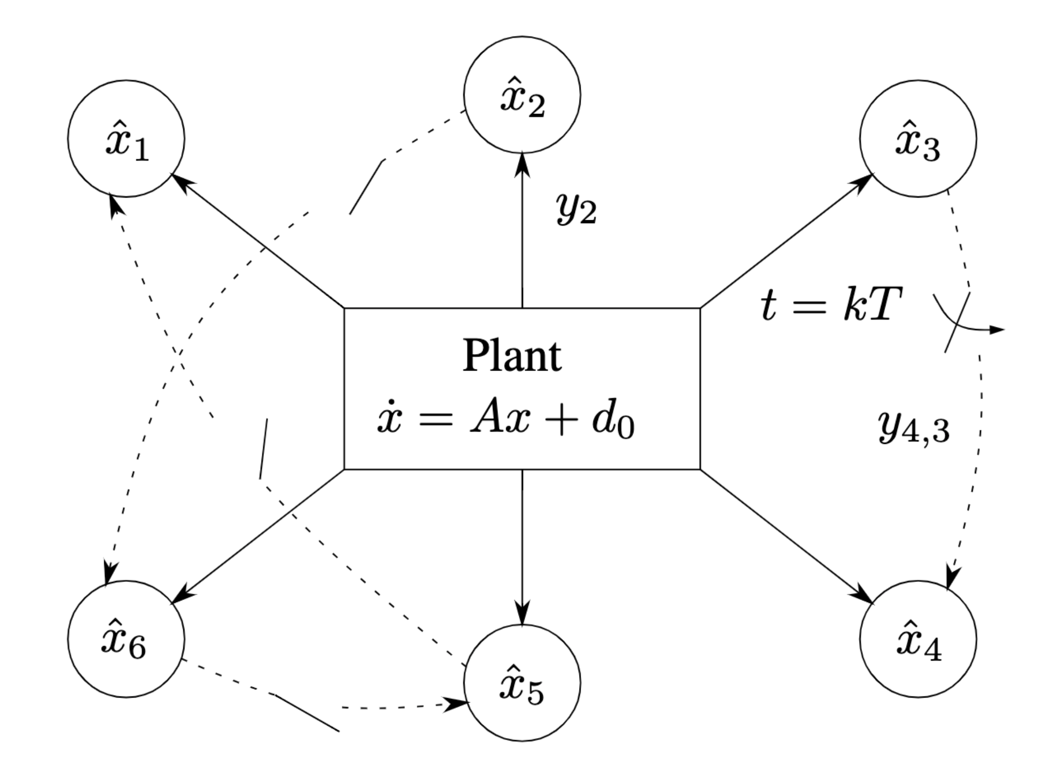
where x∈ℝnx\in\mathbb{R}^{n} is the plant state, d0d_{0} is some external disturbance, matrices AA, CiC_{i}, for all i∈𝒱i\in\mathcal{V} are constant and known. Each sensor measures an output yiy_{i} affected by measurement noise did_{i}. As shown in Fig. 1, each output measurement yi∈ℝmiy_{i}\in\mathbb{R}^{m_{i}}, with mi≤nm_{i}\leq n, is available only locally at the sensor’s location within our sensors network. Each pair (Ci,A)(C_{i},A) is not necessarily detectable.

Refer to caption
Fig. 1: Sample network with p=6p=6 sensors. Solid arrows are the locally available continuous-time measurements yiy_{i}, dashed lines are periodically sampled information exchanges among the agents.

II-B Cross-sensors information exchange

In our solution each agent is equipped with a local observer providing a state estimate x^i\hat{x}_{i}, i∈𝒱i\in\mathcal{V}. Since each measurement yiy_{i} is not necessarily sufficient for the local observer to reconstruct xx, cross-sensors communication is needed. We assume that the sensors 𝒱\mathcal{V} are connected through a communication graph 𝒢=(𝒱,ℰ)\mathcal{G}=\left(\mathcal{V},\mathcal{E}\right), wherein the exchange of information is performed synchronously and periodically with a period T>0T>0. The information exchange along each edge of the graph (i,j)∈ℰ(i,j)\in\mathcal{E} is also affected by transmission noise representing, e.g., small delays or quantization errors. Summarizing, each sensor i∈𝒱i\in{\mathcal{V}} has access to two types of measurements, namely

yi​(t),\displaystyle y_{i}(t), ∀t∈ℝ,\displaystyle\forall t\in{\mathbb{R}}, (2)
yi,j​(k​T):=x^j​(k​T)+wi,j​(k),\displaystyle y_{i,j}(kT):=\hat{x}_{j}(kT)+w_{i,j}(k), ∀k∈ℕ,∀j∈𝒩i,\displaystyle\forall k\in\mathbb{N},\forall j\in\mathcal{N}_{i}, (3)

where the second set of measurements is only available at periodic instants of time (sampled-data) tk=k​Tt_{k}=kT.

In the previous equation wi,jw_{i,j} is a (discrete-time) communication disturbance affecting the information transmitted from sensor jj to sensor ii. In the sequel, we will denote with wi:=colj∈𝒩i⁡(wi,j)w_{i}:=\col\nolimits\limits_{j\in\mathcal{N}_{i}}\left(w_{i,j}\right) the collection of the communication disturbances transmitted to sensor ii, and we will collect together all did_{i} and wiw_{i} as follows

d:=coli∈{0,…,p}⁡(di),w:=coli∈𝒱⁡(wi).\displaystyle d:=\col\nolimits\limits_{i\in\{0,\ldots,p\}}\left(d_{i}\right),\quad\quad w:=\col\nolimits\limits_{i\in\mathcal{V}}\left(w_{i}\right). (4)

II-C Problem formulation

We design here a pool of distributed observers only using the locally available information yi​(t),yi,j​(k​T)y_{i}(t),y_{i,j}(kT). Due to the disturbances acting on the plant and on the measurements, an asymptotic state estimation is not achievable. Therefore we establish an ISS bound from the disturbances (4) to the estimation errors, as stated below.

Problem 1

Design a distributed hybrid or sampled-data observer for system (1) such that, for a given exponential rate α>0\alpha>0, the following ISS property holds

|coli∈𝒱⁡(x^i​(t)−x⁡(t))|≤κ​e−α​t​|coli∈𝒱⁡(x^i​(0)−x⁡(0))|+γC​‖d‖∞+γD​‖w‖∞,∀t∈ℝ≥0,\displaystyle\begin{split}\left|\col\nolimits\limits_{i\in\mathcal{V}}\left(\hat{x}_{i}(t)-x(t)\right)\right|&\leq\kappa\mathrm{e}^{-\alpha t}\left|\col\nolimits\limits_{i\in\mathcal{V}}\left(\hat{x}_{i}(0)-x(0)\right)\right|\\ &\hskip-5.0pt+\gamma_{C}\|d\|_{\infty}+\gamma_{D}\|w\|_{\infty},\ \forall t\in\mathbb{R}_{\geq 0},\end{split} (5)

where x^i\hat{x}_{i} is the state estimate at the ii-th node and κ,γC,γD\kappa,\gamma_{C},\gamma_{D} are some strictly positive, constant gains.

Remark 1

Considering (5) without noise we obtain a standard Uniform Global Exponential Stability (UGES) property for the estimation error. Property (5) implies robustness to small nonlinearities in the plant (included in d0d_{0}) and small delays in the communication (included in wi,jw_{i,j}). More general small nonlinear perturbations of plant (1) or asynchronous communications are covered by the intrinsic robustness results in [14, Ch. 7], enabled by the well-posedness of our error dynamics. Quantitative robustness-in-the-large characterizations are more challenging objectives that will be the subject of future work.

III Continuous-discrete observer design

III-A Multi-hop decomposition and necessary assumptions

The proposed distributed observer architecture relies on the multi-hop decomposition presented in [10] for a discrete-time setting and whose main definitions are easily extended hereafter to the continuous-time case.

For the linear system (1), the ϱ\varrho-hop output matrix, Ci,ϱC_{i,\varrho}, of agent i∈𝒱i\in\mathcal{V} is recursively defined as Ci,0:=CiC_{i,0}:=C_{i} and

Ci,ϱ:=[Ci,ϱ−1colj∈𝒩i⁡(Cj,ϱ−1)].\displaystyle C_{i,\varrho}:=\begin{bmatrix}C_{i,\varrho-1}\\ \col\nolimits\limits_{j\in\mathcal{N}_{i}}\left(C_{j,\varrho-1}\right)\end{bmatrix}.

In other words, Ci,ϱC_{i,\varrho} represents the outputs measured by agent ii and by all the agents jj such that in 𝒢\mathcal{G} there exists a (directed) path from jj to ii of length at most ϱ\varrho. Consider now, for any i∈𝒱i\in\mathcal{V} and any “hop” ϱ∈{0,…,ℓi}\varrho\in\{0,\ldots,\ell_{i}\} of our multi-hop decomposition, the pair (Ci,ϱ,A)\left(C_{i,\varrho},A\right), where ℓi∈ℕ\ell_{i}\in\mathbb{N} is specified in Assumption 1 below. Based on the classical continuous-time observability concept, we can define the observable and unobservable sub-spaces of ℝn\mathbb{R}^{n} related to (Ci,ϱ,A)\left(C_{i,\varrho},A\right), denoting them by 𝒪i,ϱ\mathcal{O}_{i,\varrho} and 𝒪¯i,ϱ\overline{\mathcal{O}}_{i,\varrho}, respectively. Then, we can define the “innovation” matrix for agent ii at hop ϱ∈{0,…,ℓi}\varrho\in\{0,\ldots,\ell_{i}\} as the matrix Wi,ϱW_{i,\varrho} whose columns generate the subspace of ℝn\mathbb{R}^{n} that is observable at hop ϱ\varrho and unobservable at hop ϱ−1\varrho-1. Namely, defining 𝒪¯i,−1:=ℝn\overline{\mathcal{O}}_{i,-1}:=\mathbb{R}^{n}, Wi,ϱW_{i,\varrho} is recursively defined as an orthogonal matrix such that

Im⁡(Wi,ϱ)=𝒪¯i,ϱ−1∩𝒪i,ϱ,ϱ∈{0,…,ℓi}Im⁡(Wi,ℓi+1)=𝒪¯ℓi.\displaystyle\begin{split}&\mathrm{Im}\left(W_{i,\varrho}\right)=\overline{\mathcal{O}}_{i,\varrho-1}\cap\mathcal{O}_{i,\varrho},\quad\quad\varrho\in\{0,\ldots,\ell_{i}\}\\ &\mathrm{Im}\left(W_{i,\ell_{i}+1}\right)=\overline{\mathcal{O}}_{\ell_{i}}.\end{split} (6)

It is immediate to verify that horizontally stacking matrices Wi,ϱW_{i,\varrho} in (6), ϱ∈{0,…,ℓi+1}\varrho\in\{0,\ldots,\ell_{i}+1\}, provides an orthogonal matrix WiW_{i}, whose image is ℝn\mathbb{R}^{n}.

Remark 2

For linear systems, the observable sub-spaces related to (Ci,ϱ,A)\left(C_{i,\varrho},A\right) are identical in the continuous-time and discrete-time cases. Thus, the multi-hop decomposition results in [10, Lemma 3-10] can and will be used hereafter.

Note that matrix Wi,ℓi+1W_{i,\ell_{i}+1} in (6) might be non-empty, regardless of the value ℓi\ell_{i}. For this reason, some assumption on the unobservable modes is necessary for designing a distributed observer that solves Problem 1. In particular, given a desired exponential convergence rate α\alpha in (5), the least conservative assumption is based on the definition of collective α\alpha-detectability presented in [10].

Definition 1 (collective α\alpha-detectability [10]): Given α>0\alpha>0, system (1) is collectively α\alpha-detectable with respect to 𝒢\mathcal{G} if, for each i∈𝒱i\in\mathcal{V}, there exists ℓi∈ℕ\ell_{i}\in\mathbb{N} such that pair (Ci,ℓi,A)\left(C_{i,\ell_{i}},A\right) is α−\alpha-detectable.

Assumption 1

System (1) is collectively α\alpha-detectable with α>0\alpha>0 and ℓi\ell_{i} in (6) is selected according to Definition III-A.

Assumption 1 does not require any connectedness or spanning tree assumption on graph 𝒢\mathcal{G}, which are typical assumptions in distributed estimation. Such assumptions may be conservative (see the example in [10, Figure 1]), while it is immediate to see that Assumption 1 is necessary for solving Problem 1.

III-B Hybrid observer structure

Based on the multi-hop decomposition, each observer located at node i∈𝒱i\in\mathcal{V} is defined by the impulsive system
x^˙i=A​x^i+Wi,0​Li​(yi−C​x^i),t∉{k​T,k∈ℕ},\displaystyle\hskip-5.0pt\dot{\hat{x}}_{i}=A\hat{x}_{i}+W_{i,0}L_{i}(y_{i}-C\hat{x}_{i}),\quad t\notin\{kT,k\in{\mathbb{N}}\}, (7a)
x^i+=x^i+∑ϱ=1ℓi∑j∈𝒩iWi,ϱ​Ni,j,ϱ​Wj,ϱ−1⊤​(yi,j−x^i),t∈{k​T,k∈ℕ},\displaystyle\begin{split}&\hskip-5.0pt{\hat{x}}_{i}^{+}=\hat{x}_{i}+\sum\nolimits\limits_{\varrho=1}^{\ell_{i}}\sum\nolimits\limits_{j\in\mathcal{N}_{i}}W_{i,\varrho}N_{i,j,\varrho}W_{j,\varrho-1}^{\top}\left(y_{i,j}-\hat{x}_{i}\right),\\ &\hskip 135.0ptt\in\{kT,k\in\mathbb{N}\},\end{split} (7b)

where Wi,ϱ,i∈𝒱,ϱ∈{0,…,ℓi}W_{i,\varrho},i\in\mathcal{V},\varrho\in\{0,\ldots,\ell_{i}\} are defined in (6). The architecture of observer (7) comprises three main parts:

  1. 1.

    a continuous-time copy of the observed plant,

  2. 2.

    a local output injection, which can be performed in continuous time as well, since each sensor has access to its own measurement in continuous time,

  3. 3.

    a consensus correction term, based on the information coming from the neighbors of agent ii. Due to the communication scheme, this output injection corresponds to an impulsive modification of x^i\hat{x}_{i} in the subspace generated by matrices Wi,ϱW_{i,\varrho}, ϱ∈{1,…,ℓi}\varrho\in\{1,\dots,\ell_{i}\}.

In (7), the information coming from the neighbors is not available at all times, which makes the impulsive architecture relevant in practical implementation.

Observer (7) requires selecting matrices LiL_{i} and Ni,j,ϱN_{i,j,\varrho}, of appropriate dimension, for all (i,j,ϱ)(i,j,\varrho) in 𝒱×𝒩i×{0,…,ℓi}\mathcal{V}\times\mathcal{N}_{i}\times\{0,\dots,\ell_{i}\}. Their selection is addressed in Section III-D.

III-C Stability guarantees

The following property presents sufficient conditions for the observer in (7) to solve Problem 1. We will show in Section III-D that, under the necessary Assumption 1, there always exist observer gains satisfying this property.

Property 1

For each agent ii, the local observer gains LiL_{i} are chosen so that

A¯i,0:=(Wi,0⊤​A−Li​Ci)​Wi,0\displaystyle\overline{A}_{i,0}:=\left(W_{i,0}^{\top}A-L_{i}C_{i}\right)W_{i,0} (8)

is Hurwitz, with spectral abscissa α¯≤−α\overline{\alpha}\leq-\alpha. The consensus gains Ni,j,ϱN_{i,j,\varrho}, for all ϱ∈{1,…,ℓi}\varrho\in\left\{1,\ldots,\ell_{i}\right\}, are chosen so that

A¯i,ϱ:=e(Wi,ϱ⊤​A​Wi,ϱ)​T​(I−(∑j∈𝒩iNi,j,ϱ​Wj,ϱ−1⊤)​Wi,ϱ)\displaystyle\hskip-5.0pt\overline{A}_{i,\varrho}:=\mathrm{e}^{(W_{i,\varrho}^{\top}AW_{i,\varrho})T}\Big(I-\Big(\sum\nolimits\limits_{j\in\mathcal{N}_{i}}N_{i,j,\varrho}W_{j,\varrho-1}^{\top}\Big)W_{i,\varrho}\Big) (9)

is Schur, with spectral radius β¯∈[0,e−α​T]\overline{\beta}\in[0,\mathrm{e}^{-\alpha T}].

We are now in position to state the main result, which will be proven in Section VI-C.

Theorem 1

Given α>0\alpha>0, if the gains of observer (7) satisfy Property 1, then this observer solves Problem 1.

III-D Feasibility guarantees and design guidelines

Following [10, Th.14], we show next that Assumption 1 is not only necessary, but also sufficient for solving Problem 1.

Theorem 2

Under Assumption 1, there always exist gains LiL_{i} and Ni,j,ϱN_{i,j,\varrho} satisfying Property 1.

Proof:

The existence of matrices LiL_{i} is trivial, as (8) considers only the locally observable modes. Concerning the matrices Ni,j,ϱN_{i,j,\varrho}, we can rewrite each matrix A¯i,ϱ\overline{A}_{i,\varrho} in (9) as

A¯i,ϱ\displaystyle\overline{A}_{i,\varrho} =Ei,ϱ−N¯i,ϱ​C¯i,ϱ,\displaystyle=E_{i,\varrho}-\overline{N}_{i,\varrho}\overline{C}_{i,\varrho},

where Ei,ϱ:=eWi,ϱ⊤​A​Wi,ϱ​TE_{i,\varrho}:=\mathrm{e}^{W_{i,\varrho}^{\top}AW_{i,\varrho}T}, N¯i,ϱ:=Ei,ϱ​colj∈𝒩i​(Ni,j,ϱ⊤)⊤\overline{N}_{i,\varrho}:=E_{i,\varrho}\col\nolimits\limits_{j\in\mathcal{N}_{i}}\left(N_{i,j,\varrho}^{\top}\right)^{\top} and Ci,ϱ:=colj∈𝒩i⁡(Wj,ϱ−1⊤)​Wi,ϱC_{i,\varrho}:=\col\nolimits\limits_{j\in\mathcal{N}_{i}}\left(W_{j,\varrho-1}^{\top}\right)W_{i,\varrho}. Using this structure, we know from linear systems theory that, if the pair (C¯i,ϱ,Ei,ϱ)\left(\overline{C}_{i,\varrho},E_{i,\varrho}\right) is observable, then it is possible to find N¯i,ϱ\overline{N}_{i,\varrho} that places the eigenvalues of A¯i,ϱ\overline{A}_{i,\varrho} anywhere in the unit circle. Note also that any selection of N¯i,ϱ\overline{N}_{i,\varrho} corresponds to a unique selection of the gains Ni,j,ϱN_{i,j,\varrho} for all j∈𝒩ij\in\mathcal{N}_{i}, because Ei,ϱE_{i,\varrho} is non singular for any T>0T>0. We then complete the proof by showing observability of (C¯i,ϱ,Ei,ϱ)\left(\overline{C}_{i,\varrho},E_{i,\varrho}\right).

According to the PBH test for observability (see [15, Th.15.9]), the pair (C¯i,ϱ,Ei,ϱ)\left(\overline{C}_{i,\varrho},E_{i,\varrho}\right) is observable if and only if rank⁡([Ei,ϱ−λ​IC¯i,ϱ])=ni,ϱ,∀λ∈ℂ,\mathrm{rank}\left(\left[\begin{smallmatrix}E_{i,\varrho}-\lambda I\\ \overline{C}_{i,\varrho}\end{smallmatrix}\right]\right)=n_{i,\varrho},\;\forall\lambda\in\mathbb{C}, where the size ni,ϱn_{i,\varrho} of Ei,ϱE_{i,\varrho} corresponds to the number of columns of Wi,ϱW_{i,\varrho}. In turn, this test is true if C¯i,ϱ\overline{C}_{i,\varrho} is full column rank. From item (iii) of [10, Lemma 3] we know that the image of Wi,ϱW_{i,\varrho} is a subset of the sum of the images of Wj,ϱ−1,j∈𝒩iW_{j,\varrho-1},j\in\mathcal{N}_{i}, or equivalently

Wi,ϱ=colj∈𝒩i⁡(Wj,ϱ−1⊤)⊤​Q,\displaystyle W_{i,\varrho}=\col\nolimits\limits_{j\in\mathcal{N}_{i}}\left(W_{j,\varrho-1}^{\top}\right)^{\top}Q, (10)

where QQ is some selection matrix. Since Wi,ϱW_{i,\varrho} is full column rank by definition, we may use (10) to obtain Q⊤​C¯i,ϱ=Q⊤​colj∈𝒩i⁡(Wj,ϱ−1⊤)​Wi,ϱ=Wi,ϱ⊤​Wi,ϱQ^{\top}\overline{C}_{i,\varrho}=Q^{\top}\col\nolimits\limits_{j\in\mathcal{N}_{i}}\left(W_{j,\varrho-1}^{\top}\right)W_{i,\varrho}=W_{i,\varrho}^{\top}W_{i,\varrho}, which implies rank⁡(C¯i,ϱ)≥rank⁡(Q⊤​C¯i,ϱ)=ni,ϱ\mathrm{rank}\left(\overline{C}_{i,\varrho}\right)\geq\mathrm{rank}\left(Q^{\top}\overline{C}_{i,\varrho}\right)=n_{i,\varrho}, and since C¯i,ϱ\overline{C}_{i,\varrho} has exactly ni,ϱn_{i,\varrho} columns, the equality is immediately obtained, thus concluding the proof. ∎

Remark 3

A good practical rule is to tune the observer gains so that α¯≪−α\overline{\alpha}\ll-\alpha while β¯\overline{\beta} is closer to e−α​T\mathrm{e}^{-\alpha T}. Then the local observation errors converge to zero faster than the consensus errors, thus improving the transient behaviour.

IV Error dynamics

Define the estimation error of each agent as

ei:=x−x^i,i∈𝒱,\displaystyle e_{i}:=x-\hat{x}_{i},\quad i\in\mathcal{V}, (11)

and apply the multi-hop decomposition to the error dynamics, which yields, for each i∈𝒱i\in\mathcal{V} and each ϱ∈{0,…,ℓi+1}\varrho\in\{0,\ldots,\ell_{i}+1\}

εi,ϱ:=Wi,ϱ⊤​ei⟶ei:=∑r=0ℓi+1Wi,r​εi,r.\displaystyle\varepsilon_{i,\varrho}:=W_{i,\varrho}^{\top}e_{i}\quad\longrightarrow\quad e_{i}:=\sum\nolimits\limits_{r=0}^{\ell_{i}+1}W_{i,r}\varepsilon_{i,r}. (12)

Define also the index sets

𝒱ϱ:={i∈𝒱:ℓi+1≥ϱ},ϱ∈{0,…,ℓ¯},\displaystyle\mathcal{V}_{\varrho}:=\left\{i\in\mathcal{V}:\ell_{i}+1\geq\varrho\right\},\quad\varrho\in\{0,\ldots,\overline{\ell}\}, (13)

where ℓ¯:=maxi⁡{ℓi+1}\overline{\ell}:=\max\nolimits\limits_{i}\{\ell_{i}+1\}. Then, for each ϱ∈{0,…​ℓ¯}\varrho\in\{0,\ldots\overline{\ell}\}, we can denote with εϱ\varepsilon_{\varrho} the vector obtained by stacking all the transformed error coordinates at hop ϱ\varrho, and with ε\varepsilon the vector obtained stacking all the εϱ\varepsilon_{\varrho}, namely

εϱ:=coli∈𝒱ϱ⁡(εi,ϱ),ε:=colϱ∈{0,…,ℓ¯}⁡(εϱ)∈ℝnε.\displaystyle\varepsilon_{\varrho}:=\col\nolimits\limits_{i\in\mathcal{V}_{\varrho}}\left(\varepsilon_{i,\varrho}\right),\quad\quad\varepsilon:=\col\nolimits\limits_{\varrho\in\{0,\ldots,\overline{\ell}\}}\left(\varepsilon_{\varrho}\right)\in\mathbb{R}^{n_{\varepsilon}}. (14)

Given these definitions, the error dynamics can be described by means of a hybrid dynamical system. To this end, we augment the error state ε\varepsilon with a timer element τ\tau, which will be used to trigger periodic jumps, representing the sampled-data exchange of information. In particular, we prove in the sequel that the error dynamics results in

[ε˙τ˙]=[Aε​ε+R​d1],(ε,τ)∈𝒞,[ε+τ+]=[Jε​ε+S​w0],(ε,τ)∈𝒟,\displaystyle\hskip-10.0pt\begin{array}[]{ll}\begin{bmatrix}\dot{\varepsilon}\\ \dot{\tau}\end{bmatrix}=\begin{bmatrix}A_{\varepsilon}\varepsilon+Rd\\ 1\end{bmatrix},&(\varepsilon,\tau)\in\mathcal{C},\\ \begin{bmatrix}\varepsilon^{+}\\ \tau^{+}\end{bmatrix}=\begin{bmatrix}J_{\varepsilon}\varepsilon+Sw\\ 0\end{bmatrix},&(\varepsilon,\tau)\in\mathcal{D},\\ \end{array}

where the state evolves in X:=ℝnε×[0,T]X:=\mathbb{R}^{n_{\varepsilon}}\times\left[0,T\right] and the flow and jump sets are defined as

𝒞:=X,𝒟:={(ε,τ)∈X:τ=T}.\displaystyle\mathcal{C}:=X,\quad\quad\mathcal{D}:=\left\{(\varepsilon,\tau)\in X:\tau=T\right\}. (17)

The matrices in (IV) are defined as

Aε:=[Aℓ¯Aℓ¯−1⋆⋱0A1A0],Jε:=[Δℓ¯Δℓ¯−1⋆⋱0Δ1Δ0],\displaystyle A_{\varepsilon}:=\left[\begin{smallmatrix}A_{\overline{\ell}}&&&&\\ &A_{\overline{\ell}-1}&&\star&\\ &&\ddots&&\\ &0&&A_{1}&\\ &&&&A_{0}\end{smallmatrix}\right],\quad J_{\varepsilon}:=\left[\begin{smallmatrix}\Delta_{\overline{\ell}}&&&&\\ &\Delta_{\overline{\ell}-1}&&\star&\\ &&\ddots&&\\ &0&&\Delta_{1}&\\ &&&&\Delta_{0}\end{smallmatrix}\right], (18)
R:=colϱ∈{0,…,ℓ¯}⁡(Rϱ),S:=colϱ∈{0,…,ℓ¯}⁡(Sϱ),\displaystyle R:=\col\nolimits\limits_{\varrho\in\{0,\ldots,\overline{\ell}\}}\left(R_{\varrho}\right),\quad S:=\col\nolimits\limits_{\varrho\in\{0,\ldots,\overline{\ell}\}}\left(S_{\varrho}\right), (19)

where ⋆\star represents some possibly non-zero terms. Using the definition of 𝒱ϱ\mathcal{V}_{\varrho} in (13) and adopting the convention that the unobservable modes of node ii correspond to Ni,j,ℓi+1:=0N_{i,j,\ell_{i}+1}:=0 for all j∈𝒩ij\in\mathcal{N}_{i}, the entries of (18)-(19) are given by

Aϱ:={diagi∈𝒱⁡(Wi,0⊤​AWi,0−Li​Ci​Wi,0),if ​ϱ=0,diagi∈𝒱ϱ⁡(Wi,ϱ⊤​AWi,ϱ),if ​ϱ∈{1,…,ℓ¯},\displaystyle\hskip-7.0ptA_{\varrho}:=\begin{cases}\diag\nolimits\limits_{i\in\mathcal{V}}\left(W_{i,0}^{\top}AW_{i,0}-L_{i}C_{i}W_{i,0}\right),&\mbox{if }\varrho=0,\\ \diag\nolimits\limits_{i\in\mathcal{V}_{\varrho}}\left(W_{i,\varrho}^{\top}AW_{i,\varrho}\right),&\hskip-35.0pt\mbox{if }\varrho\in\{1,\ldots,\overline{\ell}\},\end{cases} (20a)
Rϱ:={[diagi∈𝒱⁡(−Li)|coli∈𝒱⁡(Wi,0⊤)],if ​ϱ=0,[ 0|coli∈𝒱ϱ⁡(Wi,ϱ⊤)],if ​ϱ∈{1,…,ℓ¯},\displaystyle\hskip-7.0ptR_{\varrho}:=\begin{cases}\begin{bmatrix}\diag\nolimits\limits_{i\in\mathcal{V}}\left(-L_{i}\right)\;\big|\;\col\nolimits\limits_{i\in\mathcal{V}}\left(W_{i,0}^{\top}\right)\end{bmatrix},&\mbox{if }\varrho=0,\\ \begin{bmatrix}\;\boldsymbol{0}\;\big|\;\col\nolimits\limits_{i\in\mathcal{V}_{\varrho}}\left(W_{i,\varrho}^{\top}\right)\end{bmatrix},&\hskip-30.0pt\mbox{if }\varrho\in\{1,\ldots,\overline{\ell}\},\end{cases} (20b)
Δϱ:={I,if ​ϱ=0,diagi∈𝒱ϱ⁡(I−(∑j∈𝒩iNi,j,ϱ​Wj,ϱ−1⊤)​Wi,ϱ),if ​ϱ∈{1,…,ℓ¯}.\displaystyle\hskip-7.0pt\Delta_{\varrho}:=\begin{cases}I,\hskip 125.19212pt\mbox{if }\varrho=0,\\ \diag\nolimits\limits_{i\in\mathcal{V}_{\varrho}}\left(I-\left(\sum\nolimits\limits_{j\in\mathcal{N}_{i}}N_{i,j,\varrho}W_{j,\varrho-1}^{\top}\right)W_{i,\varrho}\right),\\ \hskip 99.58464pt\mbox{if }\varrho\in\{1,\ldots,\overline{\ell}\}.\end{cases} (20c)
Sϱ:={𝟎,if ​ϱ=0,coli∈𝒱ϱ⁡(Si,ϱ),if ​ϱ∈{1,…,ℓ¯},\displaystyle\hskip-7.0ptS_{\varrho}:=\begin{cases}\boldsymbol{0},\hskip 120.0pt\mbox{if }\varrho=0,\\ \col\nolimits\limits_{i\in\mathcal{V}_{\varrho}}\left(S_{i,\varrho}\right),\hskip 50.0pt\mbox{if }\varrho\in\{1,\ldots,\overline{\ell}\},\end{cases} (20d)
Si,ϱ=−[𝟎colj∈𝒩i⁡(Wj,ϱ−1​Ni,j,ϱ⊤)⊤𝟎],\displaystyle\hskip-7.0ptS_{i,\varrho}=-\begin{bmatrix}\boldsymbol{0}\quad\col\nolimits\limits_{j\in\mathcal{N}_{i}}\left(W_{j,\varrho-1}N_{i,j,\varrho}^{\top}\right)^{\top}\quad\boldsymbol{0}\end{bmatrix}, (20e)

where the only non-zero element of the block vector Si,ϱS_{i,\varrho} is in position ii. We can finally state the following lemma, whose proof can be found in the appendix.

Lemma 1

Consider the transformed error coordinates in (12), the vector ε\varepsilon defined in (14) and the noise vectors dd and ww in (4). Then, ε\varepsilon evolves according to (IV)-(20).

Note that the flow and jump sets in (17) overlap on their boundaries. This is typical in well-posed hybrid systems [14, Ch. 6] where 𝒞\mathcal{C} and 𝒟\mathcal{D} are closed. Well-posedness ensures robustness of stability [14, Ch. 7], and even though having overlapping 𝒞\mathcal{C} and 𝒟\mathcal{D} might generate non-unique solutions, this is not a concern in the hybrid framework where Lyapunov-based proofs apply to all solutions. Moreover, uniqueness of solutions can be proved for the system (IV)-(20) and a similar situation occurs in the famous bouncing ball example [14, Ex 1.1].

V Numerical simulations

Consider the continuous-time system (1) with

A=[0100−1000000200−20],Ci=ei⊤,i∈{1,…,4},\displaystyle A=\left[\begin{smallmatrix}0&1&0&0\\ -1&0&0&0\\ 0&0&0&2\\ 0&0&-2&0\end{smallmatrix}\right],\quad\quad C_{i}=e_{i}^{\top},\quad i\in\left\{1,\ldots,4\right\},

where eie_{i} represents the ii-th vector of the Euclidean basis, i.e. a vector with all zeros and a one in position ii. The agents are interconnected with a directed ring graph, i.e. agent 1 sends information to agent 2, 2 to 3, and so on.

Refer to caption
Fig. 2: Evolution of the estimates of agent 3, compared with the plant states.
Refer to caption
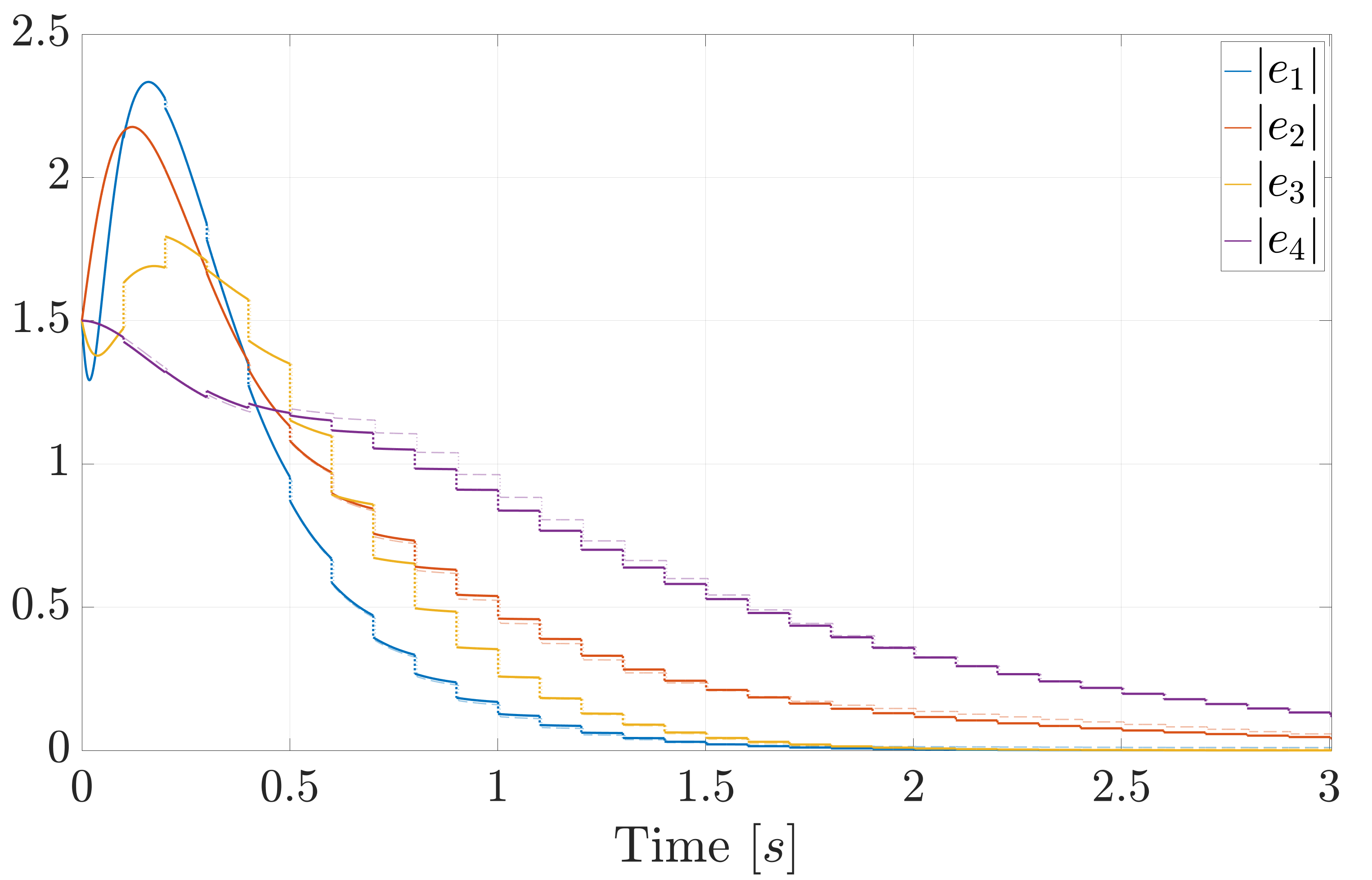
Fig. 3: Evolution of the estimation error norms: comparison between the nominal case (opaque line) and the system in presence of timer jittering (transparent line).
Refer to caption
Fig. 4: Evolution of the estimation error norms: comparison between the nominal case (opaque line) and the system in presence of transmission delays (transparent line).
Refer to caption
Fig. 5: Evolution of the estimation error norms: comparison between the nominal case (opaque line) and the system in presence of generic disturbances dd and ww, as discussed in this paper (transparent line).

We report the simulation results for the proposed observer hereafter. For this simulation, we selected T=0.1​sT=0.1s and α=1\alpha=1. The observer gains were chosen so that Property 1 was satisfied with α¯=−5​α\overline{\alpha}=-5\alpha and β¯=e−α​T\overline{\beta}=\mathrm{e}^{-\alpha T}. The disturbances dd and ww were simulated as random signals, with ‖d‖∞=0.04\|d\|_{\infty}=0.04 and ‖w‖∞=0.02\|w\|_{\infty}=0.02. In Figure 2, we can see the comparison among the state estimates of agent 3 and the plant states. We can see that the estimates of the locally observable modes, namely x^3,3\hat{x}_{3,3} and x^3,4\hat{x}_{3,4}, converge continuously to the corresponding plant states. On the other hand, convergence of the locally unavailable states x^3,1\hat{x}_{3,1} and x^3,2\hat{x}_{3,2} is achieved through the jumps emerging from the periodic information exchange with the neighbouring agents.

In Figures 3-5, the evolution of the error estimates in the nominal case is compared with three different non-ideal cases. In Figure 3, we show the result of a simulation with timer jittering, i.e. each agent is governed by its own timer state, and the information is transmitted when the value of the timer is in the interval [T−ϵτ,T+ϵτ][T-\epsilon_{\tau},T+\epsilon_{\tau}]. In this simulation, we selected ϵτ=T/10=10−2\epsilon_{\tau}=T/10=10^{-2}s. Figure 4 shows the estimation errors in the presence of communication delays, in particular the update of each agent happens with a fixed delay of δ=5⋅10−3\delta=5\cdot 10^{-3}s. Lastly, in Figure 5 we compare the nominal case with the system affected by nonzero norm-bounded Gaussian selections of dd and ww, as per our main assumption; the selected values of the infinity norms are the same as the ones used for the simulation that produced Figure 2.

VI Proof of Theorem 1

VI-A Nonsmooth Lyapunov function

Consider the Lyapunov function candidate

V⁡(ε,τ):=ε⊤​P¯​(τ)​ε:=ε⊤​eAε⊤​(T−τ)​P​eAε​(T−τ)​ε,\displaystyle\begin{split}V(\varepsilon,\tau)&\!:=\!\sqrt{\!\varepsilon^{\!\top}\overline{P}(\tau)\varepsilon}:=\sqrt{\varepsilon^{\top}\mathrm{e}^{A_{\varepsilon}^{\top}(T-\tau)}P\mathrm{e}^{A_{\varepsilon}(T-\tau)}\varepsilon},\end{split} (21)

with P>0P\!>\!0 and AεA_{\varepsilon} defined in (18) and introduce the attractor

𝒜:={(ε,τ)∈X:ε=0},\displaystyle\mathcal{A}:=\left\{(\varepsilon,\tau)\in X:\varepsilon=0\right\}, (22)

Notice that VV is smooth outside 𝒜\mathcal{A}, so we can define its gradient ∇V​(ε,τ)\nabla V(\varepsilon,\tau) for all (ε,τ)∈X∖𝒜(\varepsilon,\tau)\in X\setminus\mathcal{A}.

VI-B Properties of VV and some useful results

We will now present some properties of triangular and exponential matrices, needed to prove the main stability result. Their proofs are trivial applications of linear algebra concepts, thus they are not reported.

Lemma 2

Consider A,B∈ℝn×nA,B\in\mathbb{R}^{n\times n}. The following holds

  1. (i)

    if A,BA,B are upper triangular, then A​BAB is also upper triangular, and (a​b)i​i=ai​i​bi​i(ab)_{ii}=a_{ii}b_{ii};

  2. (ii)

    if AA is upper triangular and B=eA​tB=\mathrm{e}^{At}, then BB is also upper triangular, and bi​i=eai​i​tb_{ii}=\mathrm{e}^{a_{ii}t}

  3. (iii)

    if λ\lambda is an eigenvalue of AA, eλ​t\mathrm{e}^{\lambda t} is an eigenvalue of eA​t\mathrm{e}^{At}.

Next, we prove some properties of VV which will be used to prove the main theorem in the next section.

Proposition 1

There exist positive scalars c1c_{1}, c2c_{2}, MM, cCc_{C}, cDc_{D} and η≤e−α​T\eta\!\leq\!\mathrm{e}^{-\alpha T} such that Lyapunov function (21) verifies

  1. (i)

    c1​|ε|≤V⁡(ε,τ)≤c2​|ε|,for all ​(ε,τ)∈Xc_{1}|\varepsilon|\leq V(\varepsilon,\tau)\leq c_{2}|\varepsilon|,\quad\mbox{for all }\left(\varepsilon,\tau\right)\in X,

  2. (ii)

    |∇εV​(ε,τ)|≤M,for all ​(ε,τ)∈X∖𝒜\left|\nabla_{\varepsilon}V(\varepsilon,\tau)\right|\leq M,\quad\mbox{for all }\left(\varepsilon,\tau\right)\in X\setminus\mathcal{A},

  3. (iii)

    V˙≤cC​|d|,for all ​(ε,τ)∈𝒞∖𝒜\dot{V}\leq c_{C}|d|,\quad\mbox{for all }\left(\varepsilon,\tau\right)\in\mathcal{C}\setminus\mathcal{A},

  4. (iv)

    V+≤−η​V+cD​|w|,for all ​(ε,τ)∈𝒟∖𝒜V^{+}\leq-\eta V+c_{D}|w|,\quad\mbox{for all }\left(\varepsilon,\tau\right)\in\mathcal{D}\setminus\mathcal{A}.

Proof:

We prove the statements one by one.

Proof of (i): Since PP is positive definite, we have

λm​|eAε​(T−τ)​ε|≤V⁡(ε,τ)≤λM​|eAε​(T−τ)​ε|,\displaystyle\sqrt{\lambda_{m}}\left|\mathrm{e}^{A_{\varepsilon}(T-\tau)}\varepsilon\right|\leq V(\varepsilon,\tau)\leq\sqrt{\lambda_{M}}\left|\mathrm{e}^{A_{\varepsilon}(T-\tau)}\varepsilon\right|, (23)

where λm\lambda_{m} and λM\lambda_{M} are the minimum and maximum eigenvalues of PP, respectively. Recalling that, for any non singular matrix T∈ℝm×mT\in\mathbb{R}^{m\times m} and any vector y∈ℝmy\in\mathbb{R}^{m}, we have

|T​y|=|T−1|​|T​y||T−1|≥|T−1​T​y||T−1|=1|T−1|​|y|,\displaystyle|Ty|=\frac{|T^{-1}||Ty|}{|T^{-1}|}\geq\frac{|T^{-1}Ty|}{|T^{-1}|}=\frac{1}{|T^{-1}|}|y|,

from (23) we can obtain

c1​|ε|:=λm​ϑ1​|ε|≤V⁡(ε,τ)≤λM​ϑ2|ε|=:c2​|ε|,\displaystyle c_{1}|\varepsilon|:=\sqrt{\lambda_{m}}\vartheta_{1}|\varepsilon|\leq V(\varepsilon,\tau)\leq\sqrt{\lambda_{M}}\vartheta_{2}|\varepsilon|=:c_{2}|\varepsilon|,

where ϑ1:=minτ∈[0,T]⁡1|eAε​(τ−T)|\vartheta_{1}:=\min\nolimits\limits_{\tau\in[0,T]}\frac{1}{\left|\mathrm{e}^{A_{\varepsilon}(\tau-T)}\right|} and ϑ2:=maxτ∈[0,T]⁡|eAε​(T−τ)|,\vartheta_{2}:=\max\nolimits\limits_{\tau\in[0,T]}\left|\mathrm{e}^{A_{\varepsilon}(T-\tau)}\right|, are both strictly positive, because of continuity and since the matrix exponential is always invertible.

Proof of (ii): From the explicit calculation of the derivatives we get, for all (ε,τ)∈X∖𝒜(\varepsilon,\tau)\in X\setminus\mathcal{A},

|∇εV​(ε,τ)|=2​|P¯​ε|2​ε⊤​P¯​ε=ε⊤​P¯2​εε⊤​P¯​ε≤λM​ϑ2λm​ϑ1=:M.\displaystyle\left|\nabla_{\varepsilon}V(\varepsilon,\tau)\right|=\frac{2\left|\overline{P}\varepsilon\right|}{2\sqrt{\varepsilon^{\top}\overline{P}\varepsilon}}=\sqrt{\frac{\varepsilon^{\top}\overline{P}^{2}\varepsilon}{\varepsilon^{\top}\overline{P}\varepsilon}}\leq\frac{\lambda_{M}\vartheta_{2}}{\sqrt{\lambda_{m}}\vartheta_{1}}=:M.

Proof of (iii): Computing the evolution of VV along flows of the solutions to (IV)-(17) we get

V˙\displaystyle\dot{V} =⟨∇εV​(ε,τ),Aε​ε+R​d⟩+⟨∇τV​(ε,τ),1⟩\displaystyle=\left\langle\nabla_{\varepsilon}V(\varepsilon,\tau),A_{\varepsilon}\varepsilon+Rd\right\rangle+\left\langle\nabla_{\tau}V(\varepsilon,\tau),1\right\rangle
=2​ε⊤​P¯​Aε​ε2​ε⊤​P¯​ε+⟨∇εV​(ε,τ),R​d⟩−2​ε⊤​P¯​Aε​ε2​ε⊤​P¯​ε\displaystyle=\frac{2\varepsilon^{\top}\overline{P}A_{\varepsilon}\varepsilon}{2\sqrt{\varepsilon^{\top}\overline{P}\varepsilon}}+\left\langle{\nabla_{\varepsilon}V(\varepsilon,\tau)},Rd\right\rangle-\frac{2\varepsilon^{\top}\overline{P}A_{\varepsilon}\varepsilon}{2\sqrt{\varepsilon^{\top}\overline{P}\varepsilon}}
≤M​|R|​|d|=:cC​|d|,∀(ε,τ)∈𝒞∖𝒜.\displaystyle\leq M|R||d|=:c_{C}|d|,\hskip 50.0pt\forall(\varepsilon,\tau)\in\mathcal{C}\setminus\mathcal{A}.

Proof of (iv): For the evolution of VV across jumps of the solutions to (IV)-(17), denoting g⁡(ε,τ):=(Jε​ε+S​w, 0)g(\varepsilon,\tau):=\left(J_{\varepsilon}\varepsilon+Sw,\;0\right), we have

V+:=V⁡(g⁡(ε,w))=V⁡(g⁡(ε,0))+V⁡(g⁡(ε,w))−V⁡(g⁡(ε,0)).\displaystyle V^{+}:=V(g(\varepsilon,w))=V(g(\varepsilon,0))+V(g(\varepsilon,w))-V(g(\varepsilon,0)).

Whenever the line segment Γ:={γ​g​(ε,w)+(1−γ)​g​(ε,0),γ∈[0,1]}\Gamma:=\{\gamma g(\varepsilon,w)+(1-\gamma)g(\varepsilon,0),\gamma\in[0,1]\} does not pass through the origin, we can use the mean value theorem to rewrite V+V^{+} as

V+=V⁡(g⁡(ε,0))+⟨∇V​(ξ),g⁡(ε,w)−g⁡(ε,0)⟩,\displaystyle V^{+}=V(g(\varepsilon,0))+\left\langle\nabla V(\xi),g(\varepsilon,w)-g(\varepsilon,0)\right\rangle, (24)

for some ξ∈Γ\xi\in\Gamma. If instead 0∈Γ0\in\Gamma, then we can use a similar argument based on perturbations and converging sequences. Using (24), we obtain

V+\displaystyle V^{+} =V⁡(Jε​ε,0)+⟨∇εV​(ξ),S​w⟩+⟨∇τV​(ξ),0⟩\displaystyle=V\left(J_{\varepsilon}\varepsilon,0\right)+\left\langle\nabla_{\varepsilon}V(\xi),Sw\right\rangle+\left\langle\nabla_{\tau}V(\xi),0\right\rangle
=ε⊤​Jε⊤​eAε⊤​T​P​eAε​T​Jε​ε+⟨∇εV​(ξ),S​w⟩.\displaystyle=\sqrt{\varepsilon^{\top}J_{\varepsilon}^{\top}\mathrm{e}^{A_{\varepsilon}^{\top}T}Pe^{A_{\varepsilon}T}J_{\varepsilon}\varepsilon}+\left\langle\nabla_{\varepsilon}V(\xi),Sw\right\rangle. (25)

Consider the first term in the last line of (VI-B). Since both AεA_{\varepsilon} and JεJ_{\varepsilon} are block upper triangular, items (i) and (ii) of Lemma 2 ensure that eAε​T​Jε\mathrm{e}^{A_{\varepsilon}T}J_{\varepsilon} also is block upper triangular. Moreover, the blocks on the main diagonal of eAε​T​Jε\mathrm{e}^{A_{\varepsilon}T}J_{\varepsilon} are given by eAϱ​T​Δϱ\mathrm{e}^{A_{\varrho}T}\Delta_{\varrho}, for all ϱ∈{0,…,ℓ¯}\varrho\in\{0,\ldots,\overline{\ell}\}. Since these are in turn block diagonal matrices, we conclude that the eigenvalues of eAε​T​Jε\mathrm{e}^{A_{\varepsilon}T}J_{\varepsilon} are given by the union of the eigenvalues of the following matrices, issued from (20),

{e(Wi,0⊤​A​Wi,0−Li​Ci​Wi,0)​T,∀i∈𝒱,e(Wi,ϱ⊤​A​Wi,ϱ)​T​(I−(∑j∈𝒩iNi,j,ϱ​Wj,ϱ−1⊤)​Wi,ϱ),∀i∈𝒱,ϱ∈{1,…,ℓi},e(Wi,ℓi+1⊤​A​Wi,ℓi+1)​T,∀i∈𝒱.\displaystyle\begin{cases}\mathrm{e}^{\left(W_{i,0}^{\top}AW_{i,0}-L_{i}C_{i}W_{i,0}\right)T},\hskip 90.0pt\forall i\in\mathcal{V},\\ \mathrm{e}^{\left(W_{i,\varrho}^{\top}AW_{i,\varrho}\right)T}\left(I-\left(\sum\nolimits\limits_{j\in\mathcal{N}_{i}}N_{i,j,\varrho}W_{j,\varrho-1}^{\top}\right)W_{i,\varrho}\right),\\ \hskip 130.0pt\forall i\in\mathcal{V},\varrho\in\{1,\ldots,\ell_{i}\},\\ \mathrm{e}^{\left(W_{i,\ell_{i}+1}^{\top}AW_{i,\ell_{i}+1}\right)T},\hskip 107.0pt\forall i\in\mathcal{V}.\end{cases}

These correspond to the eigenvalues of

  • •

    eA¯i,0​T\mathrm{e}^{\overline{A}_{i,0}T} for all i∈𝒱i\in\mathcal{V},

  • •

    A¯i,ϱ\overline{A}_{i,\varrho} for all i∈𝒱,ϱ∈{1,…,ℓi}i\in\mathcal{V},\varrho\in\{1,\ldots,\ell_{i}\},

  • •

    e(Wi,ℓi+1⊤​A​Wi,ℓi+1)​T\mathrm{e}^{\left(W_{i,\ell_{i}+1}^{\top}AW_{i,\ell_{i}+1}\right)T} for all i∈𝒱i\in\mathcal{V}.

In view of Property 1, item (iii) of Lemma 2 and Assumption 1, we conclude that eAε​T​Jε\mathrm{e}^{A_{\varepsilon}T}J_{\varepsilon} has spectral radius η≤max⁡{eα¯​T,β¯,e−α​T}=e−α​T<1\eta\leq\max\{\mathrm{e}^{\overline{\alpha}T},\overline{\beta},\mathrm{e}^{-\alpha T}\}=\mathrm{e}^{-\alpha T}<1, which is equivalent to the existence of P>0P>0 such that Jε⊤​eAε⊤​T​P​eAε​T​Jε<η2​PJ_{\varepsilon}^{\top}\mathrm{e}^{A_{\varepsilon}^{\top}T}P\mathrm{e}^{A_{\varepsilon}T}J_{\varepsilon}<\eta^{2}P (see for example [15, Th. 8.4]). Then, (VI-B) becomes

V+\displaystyle V^{+} ≤η​ε⊤​P​ε+M​|S|​|w|=η​V+M​|S|​|w|=η​V+cD​|w|,\displaystyle\!\leq\eta\sqrt{\varepsilon^{\top}\!P\varepsilon}\!+\!M|S||w|=\eta V\!+\!M|S||w|=\eta\;V\!+\!c_{D}|w|,\hskip 50.0pt

for all (ε,τ)∈𝒟∖𝒜(\varepsilon,\tau)\in\mathcal{D}\setminus\mathcal{A}. ∎

VI-C Proof of Theorem 1

We will use a proof technique similar to the one in [16, Theorem 1], which needs to be carefully revisited in some of its parts, as the conditions are slightly different. For each solution ξε\xi_{\varepsilon} to (IV)-(17), we can use items (iii), (iv) of Proposition 1 to integrate the value of v⁡(t,k)=V⁡(ξε​(t,k))v(t,k)=V(\xi_{\varepsilon}(t,k)) as follows

v⁡(t,k)≤v⁡(tk,k)+cC​(t−tk)​‖d‖∞\displaystyle v(t,k)\leq v(t_{k},k)+c_{C}(t-t_{k})\|d\|_{\infty}
≤(η​v​(tk,k−1)+cD​|w|)+cC​T​‖d‖∞\displaystyle\hskip 3.0pt\leq\left(\eta v\left(t_{k},k-1\right)+c_{D}|w|\right)+c_{C}T\|d\|_{\infty}
≤η⁡(v⁡(tk−1,k−1)+cC​T​‖d‖∞)+cD​‖w‖∞+cC​T​‖d‖∞\displaystyle\hskip 3.0pt\leq\eta\left(v\left(t_{k-1},k-1\right)+c_{C}T\|d\|_{\infty}\right)+c_{D}\|w\|_{\infty}+c_{C}T\|d\|_{\infty}
≤η⁡(η​v​(tk−1,k−2)+cD​‖w‖∞)\displaystyle\hskip 3.0pt\leq\eta\left(\eta v\left(t_{k-1},k-2\right)+c_{D}\|w\|_{\infty}\right)
+cD​‖w‖∞+(1+η)​cC​T​‖d‖∞,\displaystyle\hskip 70.0pt+c_{D}\|w\|_{\infty}+\left(1+\eta\right)c_{C}T\|d\|_{\infty},

where {tk}\left\{t_{k}\right\} is the sequence of jump times of ξε\xi_{\varepsilon}, and we used the fact that 0≤(t−tk)≤T0\leq(t-t_{k})\leq T for all (t,k)∈dom​ξε(t,k)\in\mathrm{dom}\;\xi_{\varepsilon}. Iterating this process, we obtain

V⁡(ξε​(t,k))≤ηk​V​(ξε​(0,0))+∑h=0k−1ηh​cD​‖w‖∞+∑h=0kηh​T​cC​‖d‖∞.\displaystyle V(\xi_{\varepsilon}(t,k))\!\leq\!\eta^{k}V\!(\xi_{\varepsilon}(0,0))\!+\!\!\sum\nolimits\limits_{h=0}^{k-1}\!\eta^{h}\!c_{D}\!\|w\|_{\infty}\!+\!\!\sum\nolimits\limits_{h=0}^{k}\!\eta^{h}T\!c_{C}\!\|d\|_{\infty}. (26)

Recalling that η≤e−α​T\eta\leq\mathrm{e}^{-\alpha T}, we have ηk=eα​T​e−α⁡(k+1)​T≤eα​T​e−α​t\eta^{k}=\mathrm{e}^{\alpha T}\mathrm{e}^{-\alpha(k+1)T}\leq\mathrm{e}^{\alpha T}\mathrm{e}^{-\alpha t}, which, together with item (i) of Proposition 1 applied to (26), yields

|ε⁡(t,k)|≤c2c1​eα​T​e−α​t​|ε⁡(0,0)|+T​cC​‖d‖∞c1​(1−η)+cD​‖w‖∞c1​(1−η).\displaystyle|\varepsilon(t,k)|\leq\frac{c_{2}}{c_{1}}\mathrm{e}^{\alpha T}\mathrm{e}^{-\alpha t}|\varepsilon(0,0)|+\frac{Tc_{C}\|d\|_{\infty}}{c_{1}\left(1-\eta\right)}+\frac{c_{D}\|w\|_{\infty}}{c_{1}\left(1-\eta\right)}.

Lastly, we note that

|ε|2\displaystyle|\varepsilon|^{2} =∑i∈𝒱∑ϱ=0ℓi+1|Wi,ϱ⊤​ei|2=∑i∈𝒱ei⊤​Wi​∑ϱ=0ℓi+1(Qi,ϱ​Qi,ϱ⊤)​Wi⊤​ei,\displaystyle=\sum\nolimits\limits_{i\in\mathcal{V}}\sum\nolimits\limits_{\varrho=0}^{\ell_{i}+1}|W_{i,\varrho}^{\top}e_{i}|^{2}=\sum\nolimits\limits_{i\in\mathcal{V}}e_{i}^{\top}W_{i}\sum\nolimits\limits_{\varrho=0}^{\ell_{i}+1}\big(Q_{i,\varrho}Q_{i,\varrho}^{\top}\big)W_{i}^{\top}e_{i},

where each Qi,ϱQ_{i,\varrho} selects unique columns of WiW_{i}, because of the orthogonality of the multi-hop decomposition, therefore it is immediate to verify that ∑ϱ=0ℓi+1Qi,ϱ​Qi,ϱ⊤=I\sum\nolimits\limits_{\varrho=0}^{\ell_{i}+1}Q_{i,\varrho}Q_{i,\varrho}^{\top}=I. This implies |ε|2=∑i∈𝒱ei⊤​Wi​Wi⊤​ei=|coli∈𝒱⁡(ei)|2|\varepsilon|^{2}=\sum\nolimits\limits_{i\in\mathcal{V}}e_{i}^{\top}W_{i}W_{i}^{\top}e_{i}=|\col\nolimits\limits_{i\in\mathcal{V}}(e_{i})|^{2}. Therefore, we showed that (5) holds with

γC:=T​cCc1​(1−η)=T​M​|R|λm​ϑ1​(1−η)=λM​ϑ2λm​ϑ12​T​|R|1−η,\displaystyle\gamma_{C}:=\frac{Tc_{C}}{c_{1}\left(1-\eta\right)}=\frac{TM|R|}{\sqrt{\lambda_{m}}\vartheta_{1}(1-\eta)}=\frac{\lambda_{M}\vartheta_{2}}{\lambda_{m}\vartheta_{1}^{2}}\frac{T|R|}{1-\eta},
γD:=cDc1​(1−η)=λM​ϑ2λm​ϑ12​|S|1−η,κ:=c2c1​eα​T,\displaystyle\gamma_{D}:=\frac{c_{D}}{c_{1}\left(1-\eta\right)}=\frac{\lambda_{M}\vartheta_{2}}{\lambda_{m}\vartheta_{1}^{2}}\frac{|S|}{1-\eta},\qquad\kappa:=\frac{c_{2}}{c_{1}}\mathrm{e}^{\alpha T},

which completes the proof.

VII Conclusions

In this work we exploited a continuous-time formulation of the multi-hop decomposition to construct a novel distributed continuous-discrete observer. The hybrid nature of the proposed observer allowed us to analyze a scenario where the plant and the local observers work in continuous time, while the information exchange happens only periodically. Disturbances acting on the plant, on the measurements and on the communication, were also considered. Under some necessary collective detectability assumptions, we showed that it is possible to tune the observer gains to ensure exponential ISS from the noises to the estimation error, with a prescribed exponential convergence rate. Simulations were included to show the effectiveness of the proposed estimation algorithm. The extension of the proposed algorithm to aperiodic/asynchronous communications, time-varying connection graphs or nonlinear plant dynamics are interesting directions for future work. Another interesting possibility to explore is the online adaptation of the sampling period, in order to trade-off estimation performance and energy consumption.

Appendix: Proof of Lemma 1

We start by writing the flow and jump dynamics of the error coordinates. From (1) and (7), these are given by

e˙i\displaystyle\dot{e}_{i} =x˙−x^˙i=A​x+d0−A​x^i−Wi,0​Li​(yi−y^i)\displaystyle=\dot{x}-\dot{\hat{x}}_{i}=Ax+d_{0}-A\hat{x}_{i}-W_{i,0}L_{i}\left(y_{i}-\hat{y}_{i}\right)
=(A−Wi,0​Li​Ci)​ei+d0−Wi,0​Li​di\displaystyle=\left(A-W_{i,0}L_{i}C_{i}\right)e_{i}+d_{0}-W_{i,0}L_{i}d_{i}
ei+\displaystyle e_{i}^{+} =x+−x^i+\displaystyle=x^{+}-\hat{x}_{i}^{+}
=x−x^i−∑ϱ=1ℓi∑j∈𝒩iWi,ϱ​Ni,j,ϱ​Wj,ϱ−1⊤​(yi,j−x^i).\displaystyle=x-\hat{x}_{i}-\sum\nolimits\limits_{\varrho=1}^{\ell_{i}}\sum\nolimits\limits_{j\in\mathcal{N}_{i}}W_{i,\varrho}N_{i,j,\varrho}W_{j,\varrho-1}^{\top}\left(y_{i,j}-\hat{x}_{i}\right).

Then, we can use (12) to obtain

ε˙i,ϱ=Wi,ϱ⊤​A​∑r=0ϱWi,r​εi,r−Wi,ϱ⊤​Wi,0​Li​Ci​∑r=0ϱWi,r​εi,r,\displaystyle\dot{\varepsilon}_{i,\varrho}=W_{i,\varrho}^{\top}A\sum\nolimits\limits_{r=0}^{\varrho}W_{i,r}\varepsilon_{i,r}-W_{i,\varrho}^{\top}W_{i,0}L_{i}C_{i}\sum\nolimits\limits_{r=0}^{\varrho}W_{i,r}\varepsilon_{i,r},
+Wi,ϱ⊤​(d0−Wi,0​Li​di)\displaystyle\hskip 113.81102pt+W_{i,\varrho}^{\top}\left(d_{0}-W_{i,0}L_{i}d_{i}\right)
εi,ϱ+=εi,ϱ−Wi,ϱ⊤​∑r=1ℓi∑j∈𝒩iWi,r​Ni,j,r\displaystyle\varepsilon_{i,\varrho}^{+}=\varepsilon_{i,\varrho}-W_{i,\varrho}^{\top}\sum\nolimits\limits_{r=1}^{\ell_{i}}\sum\nolimits\limits_{j\in\mathcal{N}_{i}}W_{i,r}N_{i,j,r}
Wj,r−1⊤​(x^j−x^i+wi,j).\displaystyle\hskip 120.0ptW_{j,r-1}^{\top}\left(\hat{x}_{j}-\hat{x}_{i}+w_{i,j}\right).

Now, as highlighted in Remark 2, we can apply the results in [10, Lemma 3] and [10, Lemma 10], thus the flow dynamics in the previous equation becomes

ε˙i,0=(Wi,0⊤​A−Li​Ci)​Wi,0​εi,0+Wi,0⊤​d0−Li​di,\displaystyle\dot{\varepsilon}_{i,0}=\left(W_{i,0}^{\top}A-L_{i}C_{i}\right)W_{i,0}\varepsilon_{i,0}+W_{i,0}^{\top}d_{0}-L_{i}d_{i},
ε˙i,ϱ=Wi,ϱ⊤​A​∑r=0ϱWi,r​εi,r+Wi,ϱ⊤​d0,\displaystyle\dot{\varepsilon}_{i,\varrho}=W_{i,\varrho}^{\top}A\sum\nolimits\limits_{r=0}^{\varrho}W_{i,r}\varepsilon_{i,r}+W_{i,\varrho}^{\top}d_{0},

while the jump dynamics gives

εi,0+\displaystyle\varepsilon_{i,0}^{+} =εi,0,\displaystyle=\varepsilon_{i,0},
εi,ϱ+\displaystyle\varepsilon_{i,\varrho}^{+} =εi,ϱ−∑j∈𝒩iNi,j,ϱ​Wj,ϱ−1⊤​(x^j−x^i+wi,j)\displaystyle=\varepsilon_{i,\varrho}-\sum\nolimits\limits_{j\in\mathcal{N}_{i}}N_{i,j,\varrho}W_{j,\varrho-1}^{\top}\left(\hat{x}_{j}-\hat{x}_{i}+w_{i,j}\right)
=εi,ϱ−∑j∈𝒩iNi,j,ϱ​Wj,ϱ−1⊤​(∑r=0ϱWi,r​εi,rCLOSE\displaystyle=\varepsilon_{i,\varrho}-\sum\nolimits\limits_{j\in\mathcal{N}_{i}}N_{i,j,\varrho}W_{j,\varrho-1}^{\top}\bigg(\sum\nolimits\limits_{r=0}^{\varrho}W_{i,r}\varepsilon_{i,r}
OPEN−Wj,ϱ−1​εj,ϱ−1+wi,j)\displaystyle\hskip 100.0pt-W_{j,\varrho-1}\varepsilon_{j,\varrho-1}+w_{i,j}\bigg)
=εi,ϱ−∑r=0ϱ∑j∈𝒩iNi,j,ϱ​Wj,ϱ−1⊤​Wi,r​εi,r\displaystyle=\varepsilon_{i,\varrho}-\sum\nolimits\limits_{r=0}^{\varrho}\sum\nolimits\limits_{j\in\mathcal{N}_{i}}N_{i,j,\varrho}W_{j,\varrho-1}^{\top}W_{i,r}\varepsilon_{i,r}
+∑j∈𝒩iNi,j,ϱεj,ϱ−1−∑j∈𝒩iNi,j,ϱWj,ϱ−1⊤wi,j,\displaystyle\hskip 20.0pt+\sum\nolimits\limits_{j\in\mathcal{N}_{i}}N_{i,j,\varrho}\varepsilon_{j,\varrho-1}-\sum\nolimits\limits_{j\in\mathcal{N}_{i}}N_{i,j,\varrho}W_{j,\varrho-1}^{\top}w_{i,j},

which correspond to (IV) when expressed in matrix form.

References

  • [1] R. Olfati-Saber. Distributed Kalman filtering for sensor networks. In IEEE Conference on Decision and Control, pages 5492–5498, 2007.
  • [2] R. Carli, A. Chiuso, L. Schenato, and S. Zampieri. Distributed Kalman filtering based on consensus strategies. IEEE Journal on Selected Areas in Communications, 26(4):622–633, 2009.
  • [3] G. Battistelli and L. Chisci. Kullback–Leibler average, consensus on probability densities, and distributed state estimation with guaranteed stability. Automatica, 50(3):707–718, 2014.
  • [4] X. He, C. Hu, Y. Hong, L. Shi, and H. Fang. Distributed Kalman filters with state equality constraints: Time-based and event-triggered communications. IEEE Trans. on Aut. Contr., 65(1):28–43, 2019.
  • [5] F.S. Cattivelli and A.H. Sayed. Diffusion strategies for distributed kalman filtering and smoothing. IEEE Trans. on Automatic Control, 55(9):2069–2084, 2010.
  • [6] S. Kar and J.M.F. Moura. Gossip and distributed Kalman filtering: Weak consensus under weak detectability. IEEE Trans. on Signal Processing, 59(4):1766–1784, 2010.
  • [7] S. He, H.-S. Shin, S. Xu, and A. Tsourdos. Distributed estimation over a low-cost sensor network: A review of state-of-the-art. Information Fusion, 54:21–43, 2020.
  • [8] S. Park and N.C. Martins. Design of distributed LTI observers for state omniscience. IEEE Trans. on Aut. Contr., 62(2):561–576, 2016.
  • [9] A. Mitra and S. Sundaram. Distributed observers for LTI systems. IEEE Trans. on Automatic Control, 63(11):3689–3704, 2018.
  • [10] Á. Rodríguez del Nozal, P. Millán, L. Orihuela, A. Seuret, and L. Zaccarian. Distributed estimation based on multi-hop subspace decomposition. Automatica, 99:213–220, 2019.
  • [11] L. Etienne, L. Hetel, D. Efimov, and M. Petreczky. Observer synthesis under time-varying sampling for Lipschitz nonlinear systems. Automatica, 85:433–440, 2017.
  • [12] F. Ferrante, F. Gouaisbaut, R. G. Sanfelice, and S. Tarbouriech. State estimation of linear systems in the presence of sporadic measurements. Automatica, 73:101–109, 2016.
  • [13] A. Sferlazza, S. Tarbouriech, and L. Zaccarian. Time-varying sampled-data observer with asynchronous measurements. IEEE Trans. on Automatic Control, 64(2):869–876, 2018.
  • [14] R. Goebel, R.G. Sanfelice, and A.R. Teel. Hybrid Dynamical Systems: Modeling, Stability, and Robustness. Princeton University Press, 2012.
  • [15] J.P. Hespanha. Linear Systems Theory. Princeton Press, Princeton, New Jersey, 2009.
  • [16] D. Nešić, A.R. Teel, G. Valmorbida, and L. Zaccarian. Finite-gain Lp stability for hybrid dynamical systems. Automatica, 49(8):2384–2396, 2013.